Effective action model of dynamically scalarizing binary neutron stars

Abstract

Gravitational waves can be used to test general relativity (GR) in the highly dynamical strong-field regime. Scalar-tensor theories of gravity are natural alternatives to GR that can manifest nonperturbative phenomena in neutron stars (NSs). One such phenomenon, known as dynamical scalarization, occurs in coalescing binary NS systems. Ground-based gravitational-wave detectors may be sensitive to this effect, and thus could potentially further constrain scalar-tensor theories. This type of analysis requires waveform models of dynamically scalarizing systems; in this work we devise an analytic model of dynamical scalarization using an effective action approach. For the first time, we compute the Newtonian-order Hamiltonian describing the dynamics of a dynamically scalarizing binary in a self-consistent manner. Despite only working to leading order, the model accurately predicts the frequency at which dynamical scalarization occurs. In conjunction with Landau theory, our model allows one to definitively establish dynamical scalarization as a second-order phase transition. We also connect dynamical scalarization to the related phenomena of spontaneous scalarization and induced scalarization; these phenomena are naturally encompassed into our effective action approach.

I Introduction

Over a century of experiments have shown that general relativity (GR) very accurately describes the behavior of gravity. The bulk of these tests have come from measurements of gravitationally bound systems, either with electromagnetic observations of our Solar System Will (2014) and binary pulsars Wex (2014); Kramer (2016) or with gravitational-wave (GW) observations of coalescing binary black holes Abbott et al. (2016a, b, c, 2017). Combined, these systems probe GR over a large phase space, with gravitational fields whose relative strength and dynamism span many orders of magnitude Psaltis (2008); Baker et al. (2015); Berti et al. (2015); Yunes et al. (2016). However, one corner of parameter space that has not yet been directly tested is the highly-dynamical, strong-field regime of gravity coupled to matter, which would be reached in the merger of a neutron star (NS) binary system.

GWs from coalescing binary neutron stars (BNSs) are expected to be detected by Advanced LIGO in the near future Abbott et al. (2016d). Tests of GR are done using Bayesian inference Abbott et al. (2016b), comparing the relative probability that the measured data are consistent with a GR waveform over a non-GR waveform to search for possible deviations from GR. Waveforms in alternative theories of gravity can be written schematically in the Fourier domain as

$$h(\bm{\theta};f) =h_{\text{GR}}(\bm{\theta};f)\left[1+\delta\mathcal{A}(\bm{\theta};f)\right]e^{i\delta\psi(\bm{\theta};f)},$$ (1)

where $f$ is the observed GW frequency, $\bm{\theta}$ represents the intrinsic (e.g., component masses, spins, etc.) and extrinsic (e.g., distance, sky position, etc.) parameters of the binary. We have used $h_{\text{GR}}(\bm{\theta};f)$ to represent the expected waveform in GR while $\delta\mathcal{A}$ and $\delta\psi$ are the deviations in the amplitude and phase, respectively, from GR Arun et al. (2006); Yunes and Pretorius (2009); Li et al. (2012); Agathos et al. (2014). One makes an ansatz for $\delta A$ as parameterized by a set of coefficients $\left\{\alpha_{i}\right\}$ and for $\delta\psi$ as parameterized by another set of coefficients $\left\{\beta_{j}\right\}$. A common choice—the so-called restricted waveforms—is for $\delta A$ to be identically zero while, for frequencies corresponding to the inspiral, $\delta\psi$ is expanded in powers of the frequency $f$ and its logarithm $\log f$ Yunes and Pretorius (2009); Li et al. (2012); Agathos et al. (2014). For this choice, the parameters $\left\{\beta_{j}\right\}$ are simply the coefficients of the power series in $f$ and $\log f$—they measure the deviations from GR that appear at each order in a post-Newtonian (PN) expansion of the phase. Because this approach makes no reference to a particular alternative theory of gravity, constraining the parameters $\left\{\beta_{j}\right\}$ can simultaneously constrain many alternative theories using appropriate mappings.

However, this theory-agnostic approach does not capture all possible deviations from GR because it relies on the assumption that $\delta\psi(\bm{\theta};f)$ admits a series expansion in $f$ and $\log f$ during the early inspiral. In this paper, we study a particular class of scalar-tensor theories of gravity in which BNSs can undergo a phase transition known as dynamical scalarization Barausse et al. (2013); the GW signals from such systems cannot be expanded in a simple power series. Through this phenomenon, BNSs abruptly transition from a configuration that closely resembles a BNS in GR to a drastically different state. Previous efforts to model dynamically scalarizing systems have relied on phenomonological waveform models or analytic approximations of the equations of motion Sampson et al. (2014a); Palenzuela et al. (2014); Sampson et al. (2014b); Sennett and Buonanno (2016). We continue these efforts in this paper by reformulating the PN dynamics of BNSs with dynamical scalar charges in a manner analogous to the treatment of dynamical tides in GR Vines and Flanagan (2013); Steinhoff et al. (2016). Using this approach, we explicitly construct a two-body Hamiltonian that incorporates dynamical scalarization; in contrast, in Refs. Palenzuela et al. (2014); Sennett and Buonanno (2016), only the PN equations of motion were calculated. Our results comprise an important step towards fully-consistent waveform models of dynamical scalarization and offer a clear interpretation of the phenomenon as a phase transition.

The paper is organized as follows. In Sec. II, we provide an overview to scalar-tensor theories and certain nonperturbative phenomena for NSs. In Sec. III we construct an effective action to model the dynamical scalarization of BNSs. In Sec. IV we compare results obtained from our model to previous analytic approaches and numerical quasi-equilibrium (QE) configuration calculations. In Sec. V, we use our model to solidify the interpretation of dynamical scalarization as a phase transition and then discuss possible extensions to the model. Finally, we present some concluding remarks in Sec. VI.

Throughout the paper we use the conventions of Misner, Thorne, and Wheeler Misner et al. (1973) for the metric signature and Riemann tensor. We work in units in which the speed of light and the bare gravitational constant in the Einstein frame are unity.

II Nonperturbative phenomena in scalar-tensor gravity

Scalar-tensor theories of gravity are amongst the most natural and well-motivated alternatives to GR Will (2014); Berti et al. (2015). We consider the class of theories detailed in Ref. Damour and Esposito-Farese (1992), in which a massless scalar field couples nonminimally to the metric. These theories are described in the Jordan frame by the action,

$$S =\int d^{4}x\frac{\sqrt{-\tilde{g}}}{16\pi\tilde{G}}\left[\phi\tilde{R}-\frac{\omega(\phi)}{\phi}\tilde{g}^{\mu\nu}\nabla_{\mu}\phi\nabla_{\nu}\phi\right]+S_{m}[\tilde{g}_{\mu\nu},\chi],$$ (2)

where $\chi$ represents all of the matter degrees of freedom in the theory and $\tilde{G}$ is the bare gravitational coupling constant in the Jordan frame. Alternatively, the action can be written in the Einstein frame by performing a conformal transformation, $g_{\mu\nu}\equiv\phi\tilde{g}_{\mu\nu}$, as

$$S= \int d^{4}x\frac{\sqrt{-g}}{16\pi}\left[R-2g^{\mu\nu}\nabla_{\mu}\varphi\nabla_{\nu}\varphi\right]+S_{m}\left[A^{2}(\varphi)g_{\mu\nu},\chi\right],$$ (3)

where we have introduced the scalar field,

$$\varphi\equiv\int d\phi\frac{\sqrt{3+2\omega(\phi)}}{2\phi},$$ (4)

and defined

$$A(\varphi)\equiv\exp\left(-\int\frac{d\varphi}{\sqrt{3+2\omega(\varphi)}}\right).$$ (5)

Varying the Einstein-frame action yields the field equations

$$R_{\mu\nu}-\frac{1}{2}Rg_{\mu\nu} =8\pi T_{\mu\nu}+2\nabla_{\mu}\varphi\nabla_{\nu}\varphi-g_{\mu\nu}g^{\rho\sigma}\nabla_{\rho}\varphi\nabla_{\sigma}\varphi,$$ (6)

$$\square\varphi =4\pi\alpha(\varphi)T,$$ (7)

where $T^{\mu\nu}\equiv 2(-g)^{-1/2}\delta S_{m}/\delta g_{\mu\nu}$ is the stress-energy tensor of matter, $T\equiv g_{\mu\nu}T^{\mu\nu}$ is its trace, and we have introduced the coupling,

$$\alpha(\varphi)\equiv-\frac{d\log A}{d\varphi}=(3+2\omega)^{-1/2}.$$ (8)

Much of the seminal research in scalar-tensor alternatives to GR considered the simple choice of a constant coupling $\alpha$, corresponding to Jordan-Fierz-Brans-Dicke theory Jordan (1949); Fierz (1956); Brans and Dicke (1961). This theory is currently well-constrained by measurements from the Cassini probe Bertotti et al. (2003) and of binary pulsars Wex (2014); Kramer (2016); future observations by Advanced LIGO are not expected to improve these constraints Abernathy et al. (2011). Instead, in this work we consider theories whose coupling is linear in $\varphi$,

$$\alpha(\varphi)=-\beta\varphi.$$ (9)

Such theories can give rise to phenomena that are potentially detectable by Advanced LIGO while evading the bounds set by the Cassini probe Damour and Esposito-Farese (1993); Barausse et al. (2013). In particular, for sufficiently negative $\beta$, such theories can manifest spontaneous scalarization, dynamical scalarization, and induced scalarization.

Before discussing these phenomena in detail, we briefly examine the structure of NS solutions to Eqs. (6) and (7) to establish some useful notation. For simplicity, we consider a static matter source. Working far from all matter, one can expand the metric about a Minkowskian background in powers of $\epsilon\sim m_{E}/r\ll 1$ where $m_{E}$ is the total mass (measured in the Einstein frame) using the post-Minkowskian formalism (see Ref. Blanchet (2014) and references within). To leading order in $\epsilon$, Eq. (7) reduces to the Poisson equation on a flat background, whose solution in this region takes the generic form,

$$\varphi(r)=\varphi_{0}+\frac{Q}{r}+\mathcal{O}\left(\frac{1}{r^{2}}\right),$$ (10)

where we have introduced a constant background field $\varphi_{0}$ and defined the scalar charge $Q$ as the scalar monopole moment of the source.

II.1 Spontaneous scalarization

Damour and Esposito-Farèse discovered that the presence of relativistic matter in theories with negative $\beta$ can trigger an instability in the scalar field Damour and Esposito-Farese (1993). In such theories, a sufficiently compact NS can undergo a phase transition known as spontaneous scalarization corresponding to the spontaneous breaking of the symmetry $\varphi\rightarrow-\varphi$ in Eq. (3). Given current constraints from binary pulsars (see below) Antoniadis et al. (2013); Wex (2014); Shao and Wex (2016); Kramer (2016); Shao et al. (2017), numerical solutions to Eqs. (6) and (7) reveal that an isolated NS can develop a scalar charge of order

$$\frac{Q}{m_{E}}\lesssim 10^{-1},$$ (11)

through spontaneous scalarization. This figure should be contrasted with a PN prediction for this quantity,

$$\begin{split}\frac{Q}{m_{E}}&=-\beta\varphi_{0}\left(1+a_{1}C+a_{2}C^{2}+\cdots\right)\\ &\lesssim 10^{-5}\left(1+a_{1}C+a_{2}C^{2}+\cdots\right),\end{split}$$ (12)

where the coefficients $a_{i}$ are of order unity and $C\equiv m_{E}/R$ is the compactness of the NS Damour and Esposito-Farese (1992). The drastic difference in magnitude between Eqs. (11) and (12) indicates that the PN expansion does not predict spontaneous scalarization. In this sense, we describe spontaneous scalarization as nonperturbative; loosely speaking, one must include every term in the infinite sum in Eq. (12) to recover the phenomenon.

The best constraints on spontaneous scalarization come from timing measurements of white dwarf-NS binaries (see, e.g., Refs. Damour and Esposito-Farèse (1996); Freire et al. (2012); Antoniadis et al. (2013); Wex (2014); Shao and Wex (2016); Shao et al. (2017)). Unlike NSs, white dwarfs (WDs) are too diffuse to develop any significant scalar charge through spontaneous scalarization. Consequently, WD-NS binaries can emit substantial scalar dipole flux $\mathcal{F}_{\text{dip}}$, which scales as

$$\mathcal{F}_{\text{dip}}\propto\left(\frac{Q_{\text{NS}}}{m^{E}_{\text{NS}}}-\frac{Q_{\text{WD}}}{m^{E}_{\text{WD}}}\right)^{2}\approx\left(\frac{Q_{\text{NS}}}{m^{E}_{\text{NS}}}\right)^{2},$$ (13)

where $m^{E}_{\text{WD}}$ and $m^{E}_{\text{NS}}$ are the masses, and $Q_{\text{WD}}$ and $Q_{\text{NS}}$ are the scalar charges of the WD and NS, respectively. Pulsar timing experiments are sensitive to any anomalous decrease in the orbital period of the binary, and thus can constrain $\mathcal{F}_{\text{dip}}$ and consequently $Q_{\text{NS}}/m^{E}_{\text{NS}}$; we refer readers to Ref. Shao et al. (2017) for the current best limits on spontaneous scalarization from pulsar timing.

II.2 Dynamical and induced scalarization

More recently, a similar phenomenon, known as dynamical scalarization, was uncovered in numerical-relativity (NR) simulations of BNSs in the same class of scalar-tensor theories with negative $\beta$ Barausse et al. (2013); Shibata et al. (2014); Taniguchi et al. (2015). These simulations considered binary systems composed of NSs too diffuse to undergo spontaneous scalarization in isolation. As the binaries coalesced, it was found that the presence of a companion allowed the NSs to scalarize abruptly, developing scalar charges of the same order of magnitude as might occur through spontaneous scalarization. A related phenomenon, known as induced scalarization, was also discovered Barausse et al. (2013), in which a spontaneously scalarized star generates a scalar charge on a companion too diffuse to scalarize in isolation. For simplicity, we primarily focus on dynamical scalarization in this work; however, the model we develop can be applied to systems that undergo induced scalarization as well.

Numerical relativity simulations show that dynamical and induced scalarization hasten the plunge and merger of BNSs relative to the same systems in GR Barausse et al. (2013); Shibata et al. (2014). Two factors dictate the difference in merger time for scalarized versus unscalarized systems: (i) an enhancement in energy flux, and (ii) a modification to the binding energy. A scalarized BNS system will emit energy more rapidly than an unscalarized system; the dissipative channels available in GR (e.g., tensor quadrupole radiation) are enhanced for bodies with scalar charge and new channels become available (e.g., scalar dipole radiation). Modifications to the binding energy of scalarized systems are not well understood. In Ref. Taniguchi et al. (2015), the binding energy was argued to decrease (in magnitude) in scalarized systems, prompting an earlier merger, whereas in this paper, we argue that it should instead increase (see Sec. IV.2 for more detail).

Advanced LIGO will be able to distinguish between the coalescence of scalarized and unscalarized NSs provided that their scalar charges: (i) are sufficiently large and (ii) develop early enough in the inspiral (in the case of dynamical scalarization) Sampson et al. (2014a, b); Shao et al. (2017). Observation of such scalarization would provide direct evidence for modifications of GR in the strong-field regime; conversely, lack of evidence of scalarization can further constrain the space of viable scalar-tensor theories. Depending on the NS masses and equation of state (EOS) observed in coalescing BNS systems, Advanced LIGO could provide constraints competitive with current binary-pulsar limits Shao et al. (2017).

Searches for deviations from GR with GWs rely on accurate and faithful waveform models in modified gravity. Several models of dynamical scalarization have been proposed in the literature, but none at the level of sophistication of waveforms in GR. The simplest of these approaches phenomenologically model $\delta\psi(\bm{\theta};f)$ to reproduce features expected to arise in dynamically scalarized systems. For example, one can model $\delta\psi(\bm{\theta};f)$ by a polynomial in $f$ to capture effects such as scalar dipole radiation and/or use a Heaviside step function to mimic the abrupt growth of scalar charge and hastened merger triggered by dynamical scalarization. Detectability studies reveal that such models may be sufficient to identify dynamical scalarization with Advanced LIGO Sampson et al. (2014a, b). However, the accuracy of phenomenological waveform models cannot be established a priori. Ultimately, one must validate and/or calibrate these models using independent waveforms. In GR, this comparison is made with both analytic and NR waveforms (e.g., the IMRPhenom waveform family Ajith et al. (2007)). Because very few NR simulations of dynamical scalarization have been produced to date, one must rely solely on more sophisticated analytic models of this phenomenon to verify the accuracy of phenomenological models.

A more sophisticated approach towards waveform modeling, and one we shall pursue in the present work, is to solve the field equations (6) and (7) in some perturbative fashion (see Sec. III). The PN approximation is an example of such an approach; PN waveforms are useful inspiral models in their own right and also serve as the foundation for more refined waveform models, such as the effective-one-body (EOB) formalism Buonanno and Damour (1999, 2000). Dynamical scalarization can be modeled by augmenting Palenzuela et al. (2014) or resumming Sennett and Buonanno (2016) the PN dynamics in scalar-tensor gravity; such modifications are necessary because dynamical scalarization is a nonperturbative phenomenon in the same sense as spontaneous scalarization Sennett and Buonanno (2016). Both of these analytic approaches suffer from two shortcomings. First, simulating the dynamics with these models requires one to solve a system of algebraic equations at each moment in time involving the function $m_{E}(\varphi)$, which measures the complete (nonperturbative) dependence of the NS mass on the scalar field in which it is immersed. Second, these approaches only model the dynamics at the level of the equations of motion; no rigorous formulation of the two-body Hamiltonian has been constructed.

In the next section, we develop a new analytic model of dynamical scalarization that addresses these shortcomings using an effective-action approach. First, the scalar charges $Q$ are given by roots of a system of polynomial equations; for systems with no background scalar field $\varphi_{0}$, the algebraic system reduces to a pair of cubic equations that have a closed-form solution. These algebraic equations depend on only two new parameters per NS [as opposed to the complete functions $m_{E}(\varphi)$] that can be directly interpreted as the separation at which dynamical scalarization begins and the magnitude of scalar charge that develops. Second, the new model allows one to construct a simple two-body Hamiltonian and thus also compute the binding energy of a binary system. The Hamiltonian is a fundamental building block in the construction of perturbative waveform models. For example, the binding energy, in conjunction with the energy flux, allows one to compute the phase evolution through the balance equation Blanchet (2014), and the Hamiltonian is the natural starting point in constructing an EOB description of the dynamics. Additionally, our new formulation allows for a more nuanced interpretation of dynamical scalarization as a phase transition than exists in the literature and more intimately connects dynamical and spontaneous scalarization.

III Effective action with a dynamical scalar charge

We construct a model for dynamical scalarization by explicitly re-parameterizing the standard point-particle action for a BNS in terms of the scalar charges of its components. This approach closely resembles the treatment of extended bodies in GR in terms of their multipolar structure; in fact, as can be seen from Eq. (10), the scalar charge is simply the scalar monopole moment of an extended body. The gravitational fields (tensor and scalar) produced by a system of compact bodies can be represented completely in terms of the bodies’ multipoles through matched asymptotic expansions Blanchet (2014); Damour and Esposito-Farese (1992). In turn, these external fields affect the multipolar structure of the compact bodies. This response must be included into the point-particle model in some way. For example, a constant external tidal field $\mathcal{G}_{i_{1}\ldots i_{\ell}}$ will induce a multipole $\mathcal{Q}_{i_{1}\ldots i_{\ell}}$ as determined by the tidal deformability $\lambda_{\ell}$

$$\mathcal{Q}_{i_{1}\ldots i_{\ell}}=-\lambda_{\ell}\mathcal{G}_{i_{1}\ldots i_{\ell}}.$$ (14)

(See Ref. Damour and Nagar (2009) for more detail.) A more sophisticated model is needed to capture dynamical tides, i.e., tidal fields that vary on periods comparable to the relaxation timescale of the compact body (see Refs. Hinderer et al. (2016); Steinhoff et al. (2016); Flanagan and Hinderer (2008); Chakrabarti et al. (2013) and references therein).

As can be seen from the arguments of the matter action $S_{m}$ in Eq. (3), compact objects in scalar-tensor gravity interact with the scalar field in conjunction with the Einstein frame metric. For non-self-gravitating objects (i.e., test particles), this interaction is characterized simply by $A(\varphi)$. However, the internal gravitational interactions in self-gravitating objects can dramatically change the couplings to the metric and scalar field; these differences represent violations of the strong equivalence principle. As first proposed by Eardley Eardley (1975), the response of a body’s mass monopole $m_{E}$ to an external scalar field can be encoded into a generic function $m_{E}(\varphi)$. As shown in Appendix A of Ref. Damour and Esposito-Farese (1992), the scalar monopole $Q$ induced by an external scalar field is given by

$$Q=-\frac{dm_{E}}{d\varphi}.$$ (15)

For bodies immersed in weak scalar fields, Eq. (15) reduces to a linear relation analogous to Eq. (14). However dynamical scalarization occurs outside of this linear regime: the complete expression $m_{E}(\varphi)$ is needed to accurately model this phenomenon.

In this section, we develop a model inspired by the treatment of non-adiabatic tides in GR Hinderer et al. (2016); Steinhoff et al. (2016); Flanagan and Hinderer (2008); Chakrabarti et al. (2013). We rewrite the point-particle action using $Q$ in place of $\varphi$ and promote the scalar charge $Q$ to a dynamical degree of freedom. We find that this action can be expressed as a simple effective action for a dynamical scalar charge linearly coupled to an external scalar field. The complete function $m_{E}(\varphi)$ is condensed into the coupling coefficients (or “form factors”) in the effective action. Thus, the predictions of the model are parameterized by a small set of coefficients and are easy to study without reference to any particular BNS system; in contrast previous analytic models Palenzuela et al. (2014); Sennett and Buonanno (2016) required the full form of $m(\varphi)$ to be predictive.

In Sec. III.1, we develop the framework for our new effective point-particle action for a single NS and discuss possible extensions for future work. Using this approach, we compute the dynamics for a binary system of two point particles in Sec. III.2.

III.1 The effective point-particle action

We begin with the standard model of the orbital dynamics of compact objects in scalar-tensor gravity. If the orbital separation is much larger than the size of the bodies, one can represent each star as a point particle governed by an action of the form Damour and Esposito-Farese (1992, 1996, 1998),

$$S_{m}=-\int d\sigma\sqrt{-u^{\mu}u_{\mu}}m_{E}(\varphi),$$ (16)

where $z^{\mu}(\sigma)$ is the object’s worldline parametrized by a generic parameter $\sigma$, ${u^{\mu}\equiv dz^{\mu}/d\sigma}$ is its four-velocity, and $m_{E}(\varphi)$ is its Einstein-frame mass as a function of the scalar field along the worldline $\varphi(z^{\mu})$. Inserting the source (16) into Eq. (7), one finds that the compact object generates a scalar field given by

$$\Box\varphi= 4\pi\int d\sigma\frac{\sqrt{-u^{\nu}u_{\nu}}}{\sqrt{-g}}\frac{dm_{E}}{d\varphi}\delta^{(4)}(x^{\mu}-z^{\mu}),$$ (17)

where the derivative of the mass is evaluated at $\varphi(z^{\mu})$. Similarly, the influence of the object on the metric can be found by inserting Eq. (16) into Eq. (6).

Next, we convert the action (16) from a function of the external field $\varphi$ imposed on the body to one of the scalar charge $Q$. These two quantities offer complementary descriptions of the local geometry of the compact body; one can convert between the two using Eq. (15). To rewrite the action as a function of $Q$, we adopt a method first introduced in Ref. Damour and Esposito-Farèse (1996); we define a new potential $m(Q)$ given by the Legendre transformation of the mass $m_{E}(\varphi)$,

$$m(Q)\equiv m_{E}(\varphi)+Q\varphi.$$ (18)

Inserting this definition into Eq. (16), the action reads

$$S_{m}=-\int d\sigma\sqrt{-u^{\mu}u_{\mu}}\left[m(Q)-Q\varphi\right].$$ (19)

Now we promote $Q$ to an independent degree of freedom in the model; variation of the action with respect to this variable gives an additional equation of motion in the dynamics.

The notation in Eq. (18) is intentionally suggestive; as we will show in Sec. III.2, $m(Q)$ assumes the role of the particle’s mass in the orbital dynamics rather than $m_{E}(\varphi)$. A natural analogy can be drawn to thermodynamics: consider, for example, an ideal gas composed of a fixed number of particles held at a constant temperature. The state of the system can be described by either its pressure—an intrinsic quantity, analogous to $\varphi$—or its volume—an extrinsic quantity, analogous to $Q$. While the internal energy—analogous to $m_{E}(\varphi)$—has a natural interpretation as the thermal energy of the gas, it is often more convenient to use the free energy—analogous to $m(Q)$—to describe certain physical processes. As was discussed in Ref. Damour and Esposito-Farèse (1996) (and will be revisited in Sec. V), the equilibrium state for an isolated NS will minimize the function $m(Q)$; again, this quantity plays the role of an effective free energy of each NS in a binary system.

We expand the potential $m(Q)$ in a power series to quartic order,

$$m(Q)=c^{(0)}+c^{(1)}Q+\frac{c^{(2)}}{2!}Q^{2}+\frac{c^{(3)}}{3!}Q^{3}+\frac{c^{(4)}}{4!}Q^{4}+\mathcal{O}\left(Q^{5}\right).$$ (20)

Recall that the action (3) equipped with the coupling (9) is invariant under the symmetry $\varphi\rightarrow-\varphi$. Thus, we expect the mass of an isolated NS $m_{E}(\varphi)$ to also respect this symmetry, even in the presence of spontaneous scalarization. From Eq. (15), we see that this parity transformation will also send $Q\rightarrow-Q$. Performing both of these transformations leaves the right hand side of Eq. (18) unchanged, and thus we can conclude that $m(Q)$ must be an even function of $Q$.

Some of the coefficients $c^{(n)}$ have an immediate interpretation. The leading $c^{(0)}$ describes the body’s mass in absence of any scalar charge, i.e., the ADM mass in GR, and so we also denote it as $c^{(0)}=m^{(0)}$. Furthermore, a background scalar field $\varphi_{0}$ can be handled by working instead with the field,

$$\hat{\varphi}\equiv\varphi-\varphi_{0},$$ (21)

leading to an additional coupling $-Q\varphi_{0}$ in the Lagrangian. This term can be absorbed into $m(Q)$ by setting $c^{(1)}=-\varphi_{0}$, and thus we can interpret $c^{(1)}$ as a cosmologically imposed background scalar field. Note that the addition of a nonzero scalar background weakly breaks the symmetry $\varphi\rightarrow-\varphi$ in the point-particle action, prompting us to relax the conclusion that $m(Q)$ is a strictly even function. However, all other odd powers of $Q$ will still vanish, i.e., $c^{(3)}=0$.

Given the discussion above, our model for $m(Q)$ reduces to

$$m(Q)=m^{(0)}-\varphi_{0}Q+\frac{c^{(2)}}{2}Q^{2}+\frac{c^{(4)}}{24}Q^{4}+\mathcal{O}(Q^{6}).$$ (22)

Potentials of this form are widely used to describe systems that exhibit spontaneous symmetry breaking (see also Sec. V); the Higgs mechanism is one notable example Peskin and Schroeder (1995). Reference  Damour and Esposito-Farèse (1996) employed a similar potential to model isolated NSs near the critical point for spontaneous scalarization. In the present work, we show that the ansatz (22) remains valid for NSs far from this critical point; we describe the procedure by which we numerically compute the various coefficients for a particular NS in Sec. IV.1.

One ingredient conspicuously absent from our effective action (19) is the dynamical response of the scalar charges to changes in the scalar field. In truth, our model is only valid in the adiabatic limit, wherein the external fields evolve over timescales much longer than the relaxation time of NSs. Given the abrupt nature of dynamical scalarization, the validity of our assumption of adiabaticity should be studied in greater detail; we reserve this analysis for future work. If one rapidly changes the external scalar field, the NS’s scalar charge cannot respond instantaneously. In general, physical systems undergo (harmonic) oscillations around equilibrium configurations under small perturbations. Thus, one expects the scalar charge to behave approximately like a harmonic oscillator driven by the external fields, characterized by an action of the form (19) with

$$m(Q,\dot{Q})=m^{(0)}-\varphi_{0}Q+\frac{c^{(2)}}{2}\left(\frac{\dot{Q}^{2}}{\omega_{0}^{2}u^{\mu}u_{\mu}}+Q^{2}\right),$$ (23)

where $\dot{Q}=dQ/d\sigma$ and $\omega_{0}$ is the resonant frequency of this scalar mode. This action is analogous to the dynamical tidal model in Ref. Steinhoff et al. (2016): $Q$ corresponds to the dynamical quadrupole, $\varphi$ to the tidal field, $1/c^{(2)}$ to the tidal deformability, and $\omega_{0}$ to the oscillation mode frequency. In general, one should add separate dynamical degrees of freedom for every oscillation mode of the NS. Identifying all dynamical degrees of freedom relevant for the scale of interest is very important in constructing an effective action (see, e.g., Ref. Weinberg (2016)). Note that when the dynamics of the system occur much more slowly than the resonant frequency, i.e. $\dot{Q}\ll\omega_{0}$, and we restore the $Q^{4}$ interaction, Eq. (23) reduces to the adiabatic model (22) considered earlier.

Viewed from an effective field theory perspective, our effective action model of dynamical scalarization may appear too simplistic. In general, one should add to the action all possible combinations of $Q$, $u^{\mu}$, the scalar field $\varphi$, and the curvature (and derivatives of these variables) allowed by the symmetries of the theory, up to terms negligible for the desired accuracy of the model. Not all of these interactions are independent, since some might be related by redefinitions of the other dynamical variables; the redundant terms should be dropped. In the present model, we consider only couplings of the scalar charge to itself, as well as a linear coupling of the charge to the scalar field. A broader class of interactions would allow our model to reproduce other interesting phenomena. For example, the induction of scalar charges on black holes from time-varying external fields can be modeled with an effective action Jacobson (1999); Horbatsch and Burgess (2012). We delay such an investigation for future work; for the present work, the effective action model given by Eqs. (19) and (22) is sufficient to reproduce dynamical scalarization.

III.2 Dynamics of a binary system

We now turn to the task of translating the action [which will contain a copy of Eq. (19) for each NS] into a Hamiltonian describing the orbital dynamics of a BNS. Using the PN approximation, we expand the metric and scalar field in powers of $v/c$ and solve the field equations (6) and (7) at each order. An efficient method for solving the two-body dynamics is through a Fokker action together with a diagrammatic method to represent the perturbative expansion Damour and Esposito-Farese (1996). Similarly, one can integrate out the fields perturbatively using techniques from quantum field theory Goldberger and Rothstein (2006), i.e., Feynman integrals and diagrams.

We consider only the leading-order (Newtonian) approximation of the orbital dynamics in the present work. Thus, the accuracy of our model will degrade towards the end of the inspiral. However, because Advanced LIGO is only sensitive to dynamical scalarization that occurs in the very early inspiral Sampson et al. (2014a, b), our model can still be applied to the systems of scientific interest; we pursue extensions of our model to higher PN order in future work.

The PN expansions of the metric $g_{\mu\nu}$ and the scalar field $\hat{\varphi}$ are given by

$$g_{\mu\nu}= \eta_{\mu\nu}+h_{\mu\nu}+\mathcal{O}\left(c^{-4}\right),$$ (24)

$$\hat{\varphi}= \psi+\mathcal{O}\left(c^{-4}\right),$$ (25)

where $\eta_{\mu\nu}$ is the Minkowski metric and $\hat{\varphi}$ vanishes at infinity by construction. The leading-order PN corrections enter with the following powers of $c$:

$$h_{00} \sim\mathcal{O}\left(c^{-2}\right), h_{0i}\sim\mathcal{O}\left(c^{-3}\right),$$

$$h_{ij} \sim\mathcal{O}\left(c^{-4}\right), \psi\sim\mathcal{O}\left(c^{-2}\right).$$ (26)

Inserting the expansions (24) and (25) into the field equations (6) and (7) with the source (19), one finds the Newtonian-order solution to the metric and scalar field,

$$h_{00}(\mathbf{x},t) =\frac{m_{A}(Q_{A})}{|\mathbf{x}-\mathbf{z_{A}}(t)|}+\frac{m_{B}(Q_{B})}{|\mathbf{x}-\mathbf{z_{B}}(t)|}+\mathcal{O}\left(c^{-4}\right),$$ (27a)

$$\psi(\mathbf{x},t) =\frac{Q_{A}}{|\mathbf{x}-\mathbf{z_{A}}(t)|}+\frac{Q_{B}}{|\mathbf{x}-\mathbf{z_{B}}(t)|}+\mathcal{O}\left(c^{-4}\right),$$ (27b)

$$h_{0i}(\mathbf{x},t) \sim\mathcal{O}\left(c^{-3}\right),$$ (27c)

$$h_{ij}(\mathbf{x},t) \sim\mathcal{O}\left(c^{-4}\right),$$ (27d)

where the labels $A$ and $B$ distinguish the two NSs. Henceforth, we suppress the explicit dependence of each body’s mass $m$ on its corresponding scalar charge for notational convenience.

Inserting these solutions into the action and dropping singular self-interactions, we find the leading-order two-body action,

$$S\approx\int dt\bigg{[}-m_{A}-m_{B}+\frac{m_{A}}{2}\mathbf{v}_{A}^{2}+\frac{m_{B}}{2}\mathbf{v}_{B}^{2}+\frac{m_{A}m_{B}}{r}+\frac{Q_{A}Q_{B}}{r}\bigg{]},$$ (28)

where $v^{i}\equiv dz^{i}/dt$ is the Newtonian velocity and ${r\equiv|\mathbf{z}_{A}-\mathbf{z}_{B}|}$ and we have corrected for any double counting. Legendre transforming the Lagrangian yields the Hamiltonian,

$$H=m_{A}+m_{B}+\frac{\mathbf{p}_{A}^{2}}{2m_{A}}+\frac{\mathbf{p}_{B}^{2}}{2m_{B}}-\frac{m_{A}m_{B}}{r}-\frac{Q_{A}Q_{B}}{r},$$ (29)

where the canonical momenta are $\mathbf{p}_{A,B}=m_{A,B}\mathbf{v}_{A,B}$. The equation of motion for $Q_{A}$ reads

$$\begin{split}0=\frac{\partial H}{\partial Q_{A}}=z_{A}\left(-\varphi_{0}+c^{(2)}_{A}Q_{A}+\frac{c^{(4)}_{A}}{6}Q^{3}_{A}\right)-\frac{Q_{B}}{r},\end{split}$$ (30)

with the redshift given by

$$\begin{split}z_{A}=\frac{\partial H}{\partial m_{A}}=1-\frac{\mathbf{p}_{A}^{2}}{2m_{A}^{2}}-\frac{m_{B}}{r},\end{split}$$ (31)

and the equation of motion for $Q_{B}$ takes the same form but with the body labels exchanged $A\leftrightarrow B$. The scalar charges are given by the roots of these two cubic equations. Closed form solutions can be found using computer algebra for $\varphi_{0}\neq 0$, but the result is rather lengthy and not very illuminating; we do not provide them here for space considerations.

While Eq. (30) may seem daunting, simple analytic solutions for the scalar charge can be easily found in special, but very relevant cases. We restrict our attention to the theories that exactly preserve the symmetry $\varphi\rightarrow-\varphi$, i.e., we set the background scalar field $\varphi_{0}=0$. Next, for simplicity, we will neglect the $\mathcal{O}(c^{-2})$ corrections to the redshift $z_{A}$ in Eq. (30); including these terms does not change the qualitative behavior of the solutions discussed below. Finally, we specialize to the case of equal-mass binaries and assume that the NSs have identical properties, i.e. $m_{A}^{(0)}=m_{B}^{(0)}$ and $c^{(i)}_{A}=c^{(i)}_{B}$. Under these assumptions, Eq. (30) reduces to

$$0=\frac{\partial H}{\partial Q}=-2Q\left[\frac{1}{r}-c^{(2)}-\frac{c^{(4)}}{6}Q^{2}\right],$$ (32)

where we have dropped the body labels. As expected, the trivial solution $Q=0$ satisfies this equation. However, this is not necessarily the only solution; if the trivial solution is unstable, the BNS system will transition to a state with nonzero scalar charge. The requirement for stability,

$$0\leq\frac{\partial^{2}H}{\partial Q^{2}}=2c^{(2)}-\frac{2}{r}+c^{(4)}Q^{2},$$ (33)

is violated for $Q=0$ when $1/r>c^{(2)}$. The stable solutions therefore read,

$$Q=\left\{\begin{tabular}[]{lll}$0$&\quad\text{for}&$1/r\leq c^{(2)}$\\ $\pm\sqrt{\dfrac{6}{c^{(4)}}}\sqrt{\dfrac{1}{r}-c^{(2)}}$&\quad\text{for}&$1/r\geq c^{(2)}$\end{tabular}\right.,$$ (34)

which contains a phase transition at $r_{\text{DS}}=1/c^{(2)}$.

Equation (34) provides some intuition into the physical interpretation of the coefficients $c^{(2)}$ and $c^{(4)}$. The parameter $c^{(2)}$ determines the orbital scale of the phase transition to the scalarized regime, where the scalar-parity symmetry is broken and the solution bifurcates. The parameter $c^{(4)}$ determines the size of the scalar charge in this regime. Notice that for negative $c^{(2)}$ the NS is scalarized for all $r$. In fact, this situation corresponds to spontaneous scalarization; we discuss the connection between spontaneous and dynamical scalarization in greater detail in Sec. V.

Finally, we compute the Newtonian-order equations of motion for each NS. Working from the Hamiltonian (29), the equations of motion are given by,

$$\ddot{\mathbf{z}}_{A}=-\frac{m_{B}\left(1+\alpha_{A}\alpha_{B}\right)}{r^{2}}\mathbf{n},$$ (35)

where $\alpha_{A,B}\equiv Q_{A,B}/m_{A,B}$ and $\mathbf{n}\equiv(\mathbf{z}_{A}-\mathbf{z}_{B})/r$. Note that $\alpha_{A}$ differs from the quantity found in Eqs. (11)– (13) because it uses $m(Q)$ in place of $m_{E}(\varphi)$. We also derive Kepler’s third law for circular orbits

$$\Omega^{2}=\frac{\left(m_{A}+m_{B}\right)\left(1+\alpha_{A}\alpha_{B}\right)}{r^{3}},$$ (36)

where $\Omega$ is the orbital frequency.

IV Results

The previous sections aimed to motivate and develop a novel analytic model of dynamical scalarization; in this section, we test the accuracy of this approach by comparing against previous models Sennett and Buonanno (2016) and numerical QE configuration calculations Taniguchi et al. (2015). The dynamics are determined entirely by the coefficients $c^{(i)}$, as can be seen by inserting Eq. (22) and the solution of the cubic equations (30) for $Q_{A,B}$ into the Hamiltonian (29). These coefficients characterize the behavior of each compact body in isolation, and thus can be computed straightforwardly.

To facilitate comparison with previous work, we restrict our attention to the binary systems considered in Refs. Sennett and Buonanno (2016); Taniguchi et al. (2015). We consider $(1.35+1.35)\,M_{\odot}$ nonspinning BNS systems with a piecewise polytropic fit to the APR4 EOS; see Ref. Read et al. (2009) for more details on this EOS and its polytropic fit. We examine configurations with $\beta=-4.2$ and $\beta=-4.5$, where $\beta$ characterizes the strength of the scalar coupling (9). Finally, we add the background scalar field $\varphi_{0}=10^{-5}/\sqrt{-2\beta}$, which satisfies binary-pulsar constraints for this EOS Shibata et al. (2014).

IV.1 Computing $c^{(i)}$

The coefficients $c^{(i)}$ describe how the energy of an isolated NS varies with its scalar charge $Q$. Thus, to extract these coefficients, we study the behavior of the NS under infinitesimal changes in $Q$. In practice, we compute sequences of NS solutions with equal baryonic mass with incremental changes to the mass $m_{E}$, scalar charge $Q$, and asymptotic field $\varphi$. Spherically symmetric solutions for perfect fluid stars are found by solving the Tolman-Oppenheimer-Volkoff (TOV) equations; the extensions of these equations to scalar-tensor gravity were derived in Refs. Damour and Esposito-Farese (1993); Damour and Esposito-Farèse (1996). We solve these equations using fourth order Runge-Kutta methods and use standard shooting techniques to construct solutions with the same baryonic mass. The quantities $m_{E}$, $Q$, $\varphi$ parameterize the asymptotic behavior of each numerical solution; we extract $m_{E}$, $Q$, $\varphi$ using the relations detailed in Refs. Damour and Esposito-Farese (1993); Damour and Esposito-Farèse (1996). Equipped with these quantities, we then compute $m(Q)$ using Eq. (18).

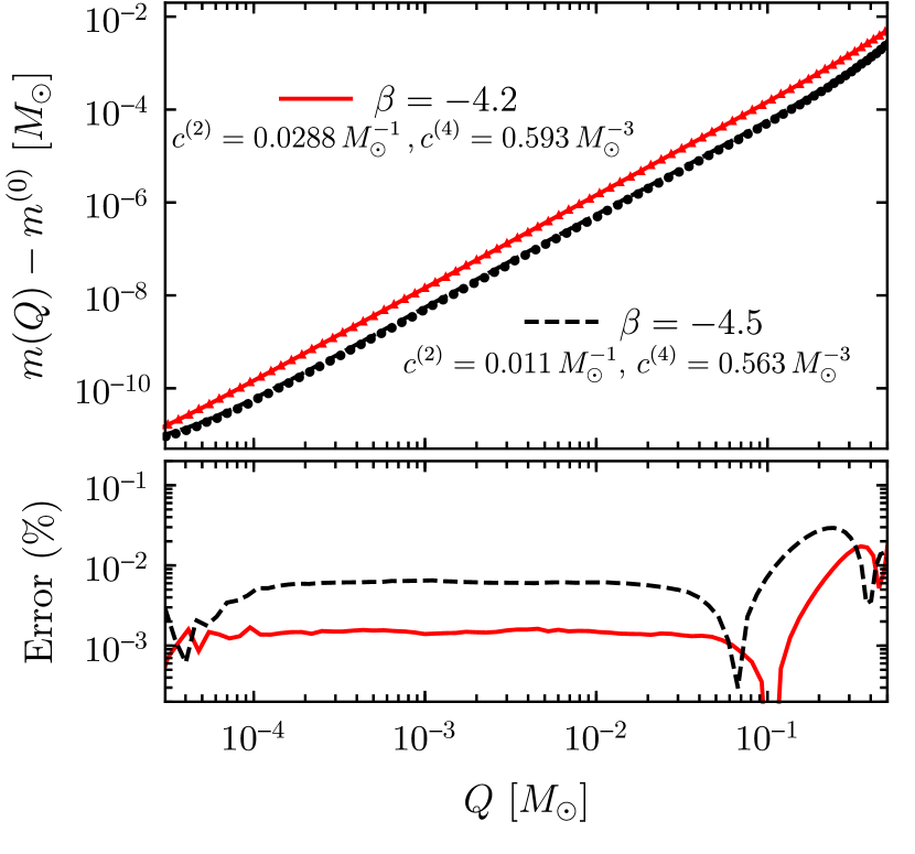
Figure 1: Potential $m$ as a function of scalar charge $Q$ for a $1.35\,M_{\odot}$ NS with the APR4 EOS. Top: The numerical values and polynomial fit are plotted with points and lines, respectively, for $\beta=-4.2$ (red) and $\beta=-4.5$ (dashed black). We have subtracted the leading-order term $m^{(0)}=1.35\,M_{\odot}$ from $m$ to improve readability. Bottom: We plot the fractional error in $m(Q)-m^{(0)}$ between the numerical data and polynomial fits.

We compute the coefficients $c^{(i)}$ by fitting the numerically computed $m(Q)$ with a polynomial of the form (22). The numerical values and polynomial fit of $m(Q)$ are plotted with dots and solid lines, respectively, in the top panel of Fig. 1 for the NS parameters discussed above. To improve readability, we have subtracted the leading-order coefficient ${m^{(0)}=1.35M_{\odot}}$ from $m$. The values for $c^{(i)}$ computed through the polynomial fit are also given in Fig. 1; the $i$-th coefficient has dimension of $\text{[mass]}^{i-1}$. The bottom panel of the figure shows the fractional error between numerical values and polynomial fits of $m-m^{(0)}$. We see that deviations are generally of the order $\lesssim 0.01\%$, slightly worsening as the charge increases. The range in $Q$ plotted here covers the typical range achievable by this NS over an entire inspiral in which dynamical scalarization occurs. As a check of our initial ansatz (22), we also fit the data to polynomials including $Q^{3}$, $Q^{5}$ and $Q^{6}$ terms; we find that these additional powers of $Q$ shift our estimates for $c^{(i)}$ by less than $\sim 0.1\%$ and only marginally improve the overall agreement to data.

IV.2 Comparison against previous models

As a first test of our model, we compute the scalar charge $Q$ as a function of frequency. Because we only consider equal-mass systems, this relation can be found by solving the cubic equation (30) for $Q=Q_{A}=Q_{B}$ as a function of separation $r$. Then, by inserting this result into Eq. (36), we determine an exact relation between $r$ and the orbital frequency $\Omega$. Finally, we invert this relation and insert it into the solution to Eq. (32) to find an implicit expression for $Q(\Omega)$. We plot $Q(\Omega)$ in Fig. 2 computed with our model in red. The lower axis gives the dimensionless orbital frequency, normalized by the total rest mass $M$, which we define as,

$$M\equiv m_{A}^{(0)}+m_{B}^{(0)},$$ (37)

i.e. the sum of the component ADM masses in GR. The upper axis gives the dominant frequency $f_{\text{GW}}=\Omega/\pi$ of the GWs produced by the binary in hertz.

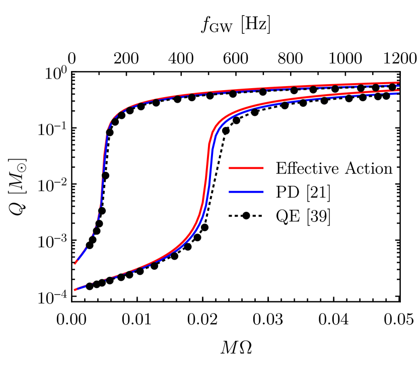
Figure 2: Scalar charge of each star as a function of frequency for a $(1.35+1.35)\,M_{\odot}$ BNS with the APR4 EOS. The lower axis indicates the orbital frequency $\Omega$; the upper axis shows the dominant GW frequency $f_{\text{GW}}=\Omega/\pi$. The model developed here using an effective action is shown in red. The analytic post-Dickean (PD) model of Ref. Sennett and Buonanno (2016) is shown in blue. The numerical calculations of quasi-equilibrium (QE) configurations performed in Ref. Taniguchi et al. (2015) are shown in black. The curves depicting earlier scalarization were computed with $\beta=-4.5$; the other set of curves correspond to $\beta=-4.2$.

We plot in blue the predictions of the post-Dickean (PD) model constructed in Ref. Sennett and Buonanno (2016). The PD approach resums the PN dynamics to reproduce dynamical scalarization. To accomplish this resummation, one promotes the mass $m_{E}$ and its derivatives to functions of two scalar fields $m_{E}(\varphi,\xi)$, Then, one field ($\varphi$) is integrated out of the point-particle action (16) through a standard PN expansion, while the other ($\xi$) is treated as a new dynamical degree of freedom in the theory. In this way, the PD approximation resembles the model presented here. Both methods introduce new degrees of freedom at the level of the action, and extremizing the action with respect to these quantities yields algebraic equations that relate the quantities to the bodies’ positions and momenta. However, in the PD approach, these equations involve the potentially complicated function $m_{E}(\varphi,\xi)$ and its derivatives, whereas in the formalism presented here, one needs only the coefficients $c^{(i)}$. In the notation of Ref. Sennett and Buonanno (2016), we define the natural analog of the scalar charge as $Q\equiv m^{(\text{RE},\varphi)}\alpha^{(\text{RE},\varphi)}/\sqrt{\phi_{0}}$ and plot this quantity in the figure; see Eqs. (A3) and (A4) in Ref. Sennett and Buonanno (2016) for the explicit definitions of these quantities. The blue curve shown in Fig. 2 corresponds to the next-to-leading-order dynamics in an expansion in $c^{-2}$.

Finally, we plot the results of the numerical QE configuration calculations performed in Ref. Taniguchi et al. (2015) with black dots. These calculations were made under the assumption of conformal flatness and stationarity; physically, each configuration represents a binary on an exactly circular orbit emitting no GWs. This setup is used to approximate a BNS during its adiabatic inspiral. The scalar mass $M_{\text{S}}$ of the total system, defined in the Jordan frame, was computed in Ref. Taniguchi et al. (2015). To convert this quantity to the scalar charge of the full system, we use $Q_{\text{tot}}=M_{\text{S}}/\left(-\beta\varphi_{0}\right)$; this conversion is discussed in detail in footnote 2 of Ref. Taniguchi et al. (2015). For simplicity, we assume that the component scalar charges are simply half of the total scalar charge, $Q=Q_{\text{tot}}/2$.

As evidenced by Fig. 2, we find very close agreement to previous predictions of the evolution of the scalar charge with our effective-action model. A key feature is the frequency $\Omega_{\text{DS}}$ at which dynamical scalarization occurs. As discussed above, our model predicts the onset of dynamical scalarization when the binary separation $r=1/c^{(2)}$. Converting the separation into an orbital frequency using Eq. (36), we find agreement to within $\lesssim 10\%$ compared to the values presented in Table II of Ref. Sennett and Buonanno (2016) for both the PD model and the QE configuration calculations. We emphasize that our effective action model is in no way calibrated to fit the QE results; the only numerical input to the model comes from isolated NS solutions of the TOV equations.

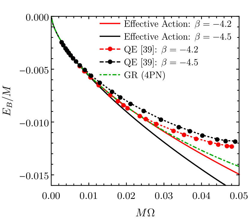
Figure 3: Binding energy $E_{B}$ normalized by the total mass $M=2.7M_{\odot}$ as a function of orbital frequency for the same BNS system as in Fig. 2. The predictions of the effective action model introduced here are shown in solid lines; we add to our Newtonian-order result the 1PN, 2PN, 3PN, and 4PN contributions found in GR. The QE configuration calculations performed in Ref. Taniguchi et al. (2015) are shown with dashed lines. Red (black) curves correspond to $\beta=-4.2$ ($\beta=-4.5$). For comparison, we have also plotted in green the 4PN prediction for the point-particle binding energy in GR.

Having computed $Q(\Omega)$, we now compute the energy of the binary system as a function of frequency. We define the binding energy $E_{B}$ of the binary as,

$$E_{B}\equiv H-M,$$ (38)

and use Eq. (29) to evaluate the Hamiltonian. Using Eq. (36) to convert $r$ to $\Omega$ we plot the binding energy (normalized by the total mass $M$) as a function of orbital frequency in Fig. 3. We also plot the binding energy computed from QE configurations in Ref. Taniguchi et al. (2015) as dashed lines and the 4PN prediction for nonspinning point particles in GR Damour et al. (2014) as a green dashed-dotted line. To improve comparison, we have added to the predictions of our effective-action model (computed at Newtonian order), the 1PN, 2PN, 3PN, and 4PN corrections to the binding energy in GR. These corrections raise the binding energy closer to the other curves in Fig. 3, but do not influence the ordering of the various curves, and thus do not affect our conclusions.

As expected, prior to the onset of dynamical scalarization, the binding energy closely resembles that of the corresponding system in GR. After dynamical scalarization occurs, we find significant differences between our analytic model and the QE results of Ref. Taniguchi et al. (2015): the present model predicts an increase in the magnitude of the binding energy $|E_{B}|$ relative to GR whereas the QE computations indicate that the magnitude should decrease. Given the interpretation of dynamical scalarization as a phase transition detailed in Sec. V, one expects the scalarized binary to be more tightly bound than the corresponding unscalarized binary, i.e., the GR prediction. If this were not the case, dynamical scalarization would be an endothermic process (requiring energy input) and the $\varphi\rightarrow-\varphi$ symmetry would not spontaneously break. Based on this intuition, the predictions of our model in Fig. 3 appear qualitatively correct. The cause of the disagreement between our model and Ref. Taniguchi et al. (2015) remains unclear. The discrepancy could stem from the assumption of conformal flatness and/or the presence of tidal interactions absent in our point-particle model of the dynamics. However, to explain the disagreement in Fig. 3, these factors would need to play a more significant role in the presence of scalar charges; analogous calculations done in GR agree with analytic point-particle predictions of the binding energy much more closely than the deviations shown in Fig. 3 (see, e.g., Ref. Taniguchi and Shibata (2010)).

V Dynamical scalarization as a phase transition

Having validated its accuracy in Sec. IV, in this section we explore an important conceptual implication of our effective action model: we definitively establish dynamical scalarization as a second-order phase transition. Using the Landau theory of phase transitions Landau (1937); *LandauTranslation, we discuss the scalarization of an isolated NS (spontaneous scalarization), an equal-mass BNS (dynamical scalarization), and an unequal-mass BNS (spontaneous, induced, and dynamical scalarization).

The approach by Landau Landau (1937); *LandauTranslation allows one to relate certain types of phase transitions to broken symmetries. We begin with a schematic review, closely following Ref. Landau (1937); *LandauTranslation. Consider a system described by a set of state variables $\bm{\zeta}$ and thermodynamic potential $\Xi(\bm{\zeta})$ that undergoes a second-order transition between two phases at some critical point $\bm{\zeta}^{*}$. The degree of symmetry in each phase can be described by an order parameter $\eta$. We choose the order parameter such that it vanishes for the phase with greater symmetry, but in the other phase, the breaking of some of these symmetries causes $\eta$ to be nonzero. To exhibit a second-order phase transition, the thermodynamic potential must admit an expansion near the critical point of the form

$$\Xi(\bm{\zeta},\eta)=\Xi_{0}(\bm{\zeta})+\Xi_{2}(\bm{\zeta})\eta^{2}+\Xi_{4}(\bm{\zeta})\eta^{4}+\mathcal{O}\left(\eta^{6}\right),$$ (39)

where the coefficients obey the following conditions:

$$\Xi_{4}(\bm{\zeta})> 0,$$ (40)

$$\Xi_{2}(\bm{\zeta}^{*})= 0.$$ (41)

The first condition guarantees that the system has an equilibrium solution (found at the minimum of $\Xi$). We discuss the second condition below.

For states “above” $\bm{\zeta}^{*}$, i.e., those for which $\Xi_{2}(\bm{\zeta})>0$, the potential (39) is positive definite, and so the system reaches equilibrium in the more symmetric state (the one in which $\eta$ vanishes). However, as one passes through the point $\bm{\zeta}^{*}$, the coefficient $\Xi_{2}(\bm{\zeta})$ changes sign; now the potential (39) is minimized for configurations with nonzero values of $\eta$.

In anticipation of later discussion, we generalize the treatment above to systems described by a vector order parameter $\bm{\eta}\in\mathbb{R}^{n}$, where Euclidean coordinates are denoted with unitalicized Latin indices. In this generalization, the functions $\Xi_{m}(\bm{\zeta})$ become rank-$m$ tensors of dimension $n$ such that Eq. (39) becomes

$$\begin{split}\Xi(\bm{\zeta},\bm{\eta})=&\Xi_{0}(\bm{\zeta})+\left[\Xi_{2}(\bm{\zeta})\right]_{\text{ab}}\eta^{\text{a}}\eta^{\text{b}}+\left[\Xi_{4}(\bm{\zeta})\right]_{\text{abcd}}\eta^{\text{a}}\eta^{\text{b}}\eta^{\text{c}}\eta^{\text{d}}\\ &+{\cal O}\left(\bm{\eta}^{6}\right).\end{split}$$ (42)

The conditions (40) and (41) must be appropriately extended, as well. To ensure that the system has an equilibrium solution, we require that $\Xi_{4}$ be positive definite, in the sense that

$$\left[\Xi_{4}(\bm{\zeta})\right]_{\text{abcd}}\eta^{\text{a}}\eta^{\text{b}}\eta^{\text{c}}\eta^{\text{d}}>0,\qquad\forall\,{\bm{\eta}}\in\mathbb{R}^{n}.$$ (43)

The $n$-dimensional generalization of Eq. (41) is

$$\det\left(\left[\Xi_{2}(\bm{\zeta}^{*})\right]_{\text{ab}}\right)=0.$$ (44)

Note that in the phase with greater symmetry, our assumption that $\Xi$ is minimized when $\bm{\eta}$ vanishes ensures that all eigenvalues of the matrix $\left[\Xi_{2}(\bm{\zeta}^{*})\right]_{\text{ab}}$ must be positive. In the less symmetric phase, at least one of the eigenvalues must be negative; however, the determinant of the matrix remains positive if an even number of eigenvectors have negative eigenvalues.

V.1 Spontaneous scalarization of an isolated body

The classical illustration of a second-order phase transition is spontaneous magnetization in a ferromagnet at the Curie temperature $T_{C}$. In this example, $\Xi$ is the energy $E$ of the system and $\bm{\zeta}$ represents the temperature and external magnetic field $\bm{B}$. The order parameter $\eta$ is the total magnetization $\bm{M}\equiv-\partial E/\partial\bm{B}$, which is thermodynamically conjugate to $\bm{B}$. Inspired by this example, Damour and Esposito-Farèse (1996) considered a phenomenological model of spontaneous scalarization following the Landau ansatz (39). Starting from the total energy of an isolated NS $m_{E}(\varphi)$, the authors selected the potential $m(Q)$, defined as in Eq. (18), to play the role of $\Xi$. The bulk properties of the NS are its baryonic mass $\bar{m}$ and external scalar field $\varphi$. Analogous to spontaneous magnetization, the authors identified the order parameter $Q$ as the conjugate variable to the scalar field [c.f. Eq. (15)]. The behavior of the potential $m$ around the critical baryonic mass $\bar{m}_{\text{cr}}$ was modeled by Damour and Esposito-Farèse (1996)

$$m(Q)=\frac{1}{2}a\left(\bar{m}_{\text{cr}}-\bar{m}\right)Q^{2}+\frac{1}{4}bQ^{4},$$ (45)

where $a$ and $b$ are constant (positive) coefficients. Above the critical baryonic mass, NSs equilibrate in configurations with nonzero scalar charge.

By design, our point-particle model (22) takes the same form as Eq. (45), and thus can model spontaneous scalarization as well. Unlike Eq. (45), we do not factor out any mass-dependence of the coefficients $c^{(i)}$. As demonstrated in Section IV.1, our model remains valid for stars with $\bar{m}\not\approx\bar{m}_{\text{cr}}$—these stars were not considered in Ref.  Damour and Esposito-Farèse (1996). The coefficient $c^{(2)}$ plays the role of $\Xi_{2}$ in the Landau ansatz (39); note that this coefficient depends on the properties of the NS (e.g., the mass and EOS) and on the scalar-tensor coupling (characterized by $\beta$). The critical point at which a NS transitions from an unscalarized state ($Q=0$) to a spontaneously scalarized state ($Q\neq 0$) occurs when $c^{(2)}$ is zero. Neutron stars with negative values of $c^{(2)}$ must spontaneously scalarize; the unscalarized state is unstable.

V.2 Dynamical scalarization of equal-mass binaries

With our effective action model, we can now apply this analysis to a binary system of NSs. For simplicity, we begin by studying equal-mass systems with zero background scalar field $\varphi_{0}$. We assume that NSs have the same properties as well, i.e., $c^{(i)}_{A}=c^{(i)}_{B}$. For illustrative purposes, we drop the $\mathbf{p}^{2}$ and $m/r$ terms in the Hamiltonian (29); restoring these terms does not affect the qualitative behavior we describe below.

Under these assumptions, the Hamiltonian is given by

$$H=2m^{(0)}+\left(c^{(2)}-\frac{1}{r}\right)Q^{2}+\frac{c^{(4)}}{12}Q^{4},$$ (46)

where we have dropped the body labels. This expression takes the same form as Eq. (39). Using the same analysis as in the previous subsection, we show that dynamical scalarization is a second-order phase transition that occurs at a separation ${r_{\text{DS}}=1/c^{(2)}}$; this conclusion agrees with our prediction in Eq. (34). By comparing Eqs. (22) and (46) we see that an equal-mass dynamically scalarizing system behaves like an isolated NS with an effective coefficient $c^{(2)}_{\text{eff}}\equiv c^{(2)}-1/r$ that decreases as the binary coalesces.

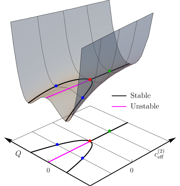
Figure 4: Illustration of the Hamiltonian of an equal-mass BNS as function of scalar charge and effective coefficient $c^{(2)}_{\text{eff}}=c^{(2)}-1/r$. Solutions to the equations of motion are highlighted with solid lines. When $c^{(2)}_{\text{eff}}$ becomes negative, the trivial solutions $Q=0$ become unstable. The bottom lower plane shows the projection of the solutions.

In Fig. 4, we plot the simplified Hamiltonian  (46) as a function of charge and effective coefficient $c^{(2)}-1/r$. For positive values of this effective coefficient, the energy is minimized in the trivial configuration $Q=0$. Below the critical point $c^{(2)}_{\text{eff}}=0$, the unscalarized state becomes unstable; instead, the binary system transitions into a scalarized state. The bottom plane shows the projection of the equilibrium solutions in black. As predicted by Eq.  (34), the stable solutions bifurcate at the critical point, spontaneously breaking the scalar-parity symmetry of the theory. Note that this entire discussion can be applied directly to isolated NSs that undergo spontaneous scalarization by taking $r\rightarrow\infty$.

V.3 Scalarization of unequal-mass binaries

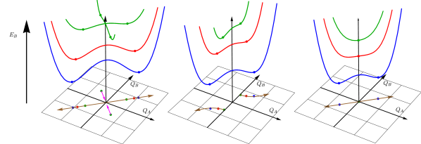
Figure 5: Illustration of the binding energy as a function of scalar charge for BNSs that undergo: (left) spontaneous scalarization, (middle) induced scalarization, and (right) dynamical scalarization. Equilibrium solutions are highlighted with dots. The solutions are projected onto the $(Q_{A},Q_{B})$ plane below; colored arrows indicate the flow of these solutions as the binary coalesces.

Finally, we turn our attention to the critical phenomena that can occur in unequal-mass binaries. The (vector) order parameter $\bm{\eta}\in\mathbb{R}^{2}$ is given by

$$(\eta^{1},\eta^{2})=(Q_{A},Q_{B})\,.$$ (47)

Again, we assume that the background scalar field $\varphi_{0}$ vanishes and drop the $\mathbf{p}^{2}$ and $m/r$ terms in the Hamiltonian (29); these simplifications do not affect the qualitative behavior described below. Under these assumptions, the Hamiltonian takes the same form as Eq. (42) with

$$\Xi_{0}= m_{A}^{(0)}+m_{B}^{(0)},$$ (48)

$$\left[\Xi_{2}\right]_{\text{ab}}= \frac{1}{2}\begin{pmatrix}c_{A}^{(2)}&-r^{-1}\\ -r^{-1}&c_{B}^{(2)}\end{pmatrix},$$ (49)

$$\left[\Xi_{4}\right]_{\text{abcd}}= \frac{1}{24}\left(c_{A}^{(4)}\delta_{\text{a}}^{1}\delta_{\text{b}}^{1}\delta_{\text{c}}^{1}\delta_{\text{d}}^{1}+c_{B}^{(4)}\delta_{\text{a}}^{2}\delta_{\text{b}}^{2}\delta_{\text{c}}^{2}\delta_{\text{d}}^{2}\right).$$ (50)

We examine the Hamiltonian (29) for systems that undergo:

1. Spontaneous scalarization: Both stars are initially scalarized $(c^{(2)}_{A}<0,\,c^{(2)}_{B}<0)$,

2. Induced scalarization: Only one star is initially scalarized $(c^{(2)}_{A}>0,\,c^{(2)}_{B}<0)$,

3. Dynamical scalarization: Neither star is initially scalarized $(c^{(2)}_{A}>0,\,c^{(2)}_{B}>0)$.

For all three cases, we restrict our attention to binaries following circular orbits. The binding energy is shown in Fig. 5 as a function of the NS charges. We show only the slices of the full graph $E_{B}(Q_{A},Q_{B})$ that pass through equilibrium solutions; for comparison, these curves correspond to the thin black lines on the surface in Fig. 4. Moving from left to right, the plots correspond to spontaneous, induced, and dynamical scalarization, respectively. Moving downwards in each plot, the green, red, and blue curves depict the binding energy at progressively smaller separations. The equilibrium solutions are denoted with dots on the curves and are projected onto the $(Q_{A},Q_{B})$-plane in the color corresponding to their separation. The colored arrows depict the flow of equilibrium solutions as the separation decreases.

At large separations (green), there exist four stable configurations for spontaneously scalarized binaries (left panel): each NS can exhibit a positive or negative scalar charge, and the choices for each are uncorrelated. However, as the separation decreases (red and blue), configurations in which the two stars have opposite-parity charges become energetically unfavorable. As indicated by the pink arrows, these solutions flow towards the origin and transform into a saddle point, i.e., this branch of solutions becomes unstable. Thus, at this critical separation (red) there exists a new phase transition distinct from those discussed above. From Eqs. (44) and (49), we find that this critical point occurs at a separation of $r^{*}=(c_{A}^{(2)}c_{B}^{(2)})^{-1/2}$. Unlike with dynamical scalarization, the more symmetric state phase occurs at separations smaller than $r^{*}$. The equilibrium solutions with charges of the same sign flow away from the origin as the binary coalesces. The charge of each spontaneously scalarized star will continue to grow during the inspiral due to feedback from its companion.

Binaries that undergo induced scalarization (middle panel) begin with an unscalarized star $Q_{A}=0$ and a scalarized star $Q_{B}\neq 0$ (green). As the stars are brought closer together (red), the unscalarized star rapidly develops scalar charge, whereas the initially scalarized star remains (approximately) unchanged. However, as the separation decreases further (blue), the two charges become of the same order of magnitude and continue to increase at roughly the same rate through the remainder of the coalescence. Unlike for spontaneous and dynamical scalarization, the branches of equilibrium solutions are disjoint throughout the entire coalescence, i.e. the colored arrows in Fig. 5 never meet. Because $c_{A}^{(2)}$ and $c_{B}^{(2)}$ have opposite signs, the determinant of $\left[\Xi_{2}\right]_{\text{ab}}$ [given in Eq. (49)] is negative for all separations. Induced scalarization fails to meet condition (44) and therefore cannot be classified as a phase transition.

Finally, initially unscalarized unequal-mass binaries (right panel) evolve similarly as in Fig. 4. As seen in Fig. 5, the binary system begins in an unscalarized state (green). At the critical transition point (red), the effective $c^{(2)}$ coefficient vanishes; beyond that point (blue), scalarization becomes energetically favorable. Again, Eqs. (44) and (49) reveal that dynamical scalarization occurs at a separation of $r_{\text{DS}}=(c_{A}^{(2)}c_{B}^{(2)})^{-1/2}$, which reduces to the result in Sec. V.2 when $c_{A}^{(2)}=c_{B}^{(2)}$. As before, the scalar charges continue to grow after the onset of dynamical scalarization.

VI Conclusions

In the present paper, we developed a new point-particle model for NSs in scalar-tensor gravity that can reproduce spontaneous, induced, and dynamical scalarization. The model parametrizes the various scalarization phenomena by just two coefficients $c^{(2)}$, $c^{(4)}$ for each NS. This approach should be contrasted with previous analytic models of dynamical scalarization  Palenzuela et al. (2014); Sennett and Buonanno (2016), which relied upon numerically solving equations containing the generic function $m_{E}(\varphi)$. For the first time, we have computed a two-body Hamiltonian that incorporates dynamical scalarization in a self-consistent manner (see Ref. Sennett and Buonanno (2016) for a discussion of previous attempts). Observables derived from the model at leading order in the PN expansion were shown to be in good agreement with earlier analytic models and numerical QE calculations. The identification of the relevant dynamical variables in the effective action is crucial to our model.

Analogous to the analysis done in Ref. Damour and Esposito-Farèse (1996) concerning spontaneous scalarization, our model rigorously establishes dynamical scalarization as a phase transition as per Landau theory Landau (1937); *LandauTranslation. Additionally, it demonstrates the intimate connection between spontaneous and dynamical scalarization. The mapping between an equal-mass BNS undergoing dynamical scalarization and an effective spontaneously scalarized NS is detailed in Sec. V.2.

Our effective action stands as an important first step towards accurate analytic waveforms of dynamically scalarizing BNSs. The model benefits from its close analogy to the effective action model of dynamical tides detailed in Refs. Hinderer et al. (2016); Steinhoff et al. (2016)—the dynamical scalar monopole $Q$ here corresponds to the dynamical gravitational quadrupole therein. References Hinderer et al. (2016); Steinhoff et al. (2016) derived an accurate EOB Buonanno and Damour (1999, 2000) waveform model incorporating dynamical tidal interactions. Using this model as a template, one could construct an analogous model for dynamical scalar-tensor effects. This construction will require calculations of dissipative effects and higher PN order results for the conservative dynamics.

Another avenue for future work is the addition of kinetic-energy terms to the effective action as in Eq. (23). Resonant effects play an important role in the dynamical tides model of Refs. Hinderer et al. (2016); Steinhoff et al. (2016); it remains to be seen whether analogous effects could be important with dynamical scalar charges. Formulating the effective action in this manner offers a conceptual advantage over the current model, as it guarantees that all of the equations of motion are ordinary differential equations (rather than a mix of nonlinear algebraic and differential equations).

Finally, an intriguing extension of this work is to theories with a massive scalar field. Pulsar timing cannot constrain sufficiently short-range scalar fields, so a much wider range of parameter space of massive scalar-tensor theories remains to be constrained by GW observations than that of theories with a massless scalar Ramazanoglu and Pretorius (2016). The PN dynamics of a simple massive scalar-tensor theory were investigated in Ref. Alsing et al. (2012), and spontaneous scalarization of isolated NSs was studied in Refs. Ramazanoglu and Pretorius (2016); Yazadjiev et al. (2016); the framework we have presented above could synthesize these results with appropriate modifications to the field equations (6) and (7).