An equilibrium-conserving taxation scheme for income from capital

Abstract

Under conditions of market equilibrium, the distribution of capital income follows a Pareto power law, with an exponent that characterizes the given equilibrium. Here, a simple taxation scheme is proposed such that the post-tax capital income distribution remains an equilibrium distribution, albeit with a different exponent. This taxation scheme is shown to be progressive, and its parameters can be simply derived from (i) the total amount of tax that will be levied, (ii) the threshold selected above which capital income will be taxed and (iii) the total amount of capital income. The latter can be obtained either by using Piketty’s estimates of the capital/labor income ratio or by fitting the initial Pareto exponent. Both ways moreover provide a check on the amount of declared income from capital.

I Introduction

The distribution of income has been studied for a long time in the economic literature, and has more recently become a topic of investigation for statistical physicists turning to econophysics Chak1 ; Chak2 ; Yakovenko ; Chak3 . The income distribution is characterized by a density function $f(x)$ such that $f(x)dx$ is the number of individuals earning income between $x$ and $x+dx$. From the empirical data obtained from tax records, two different regimes are readily distinguished. For income levels below a certain threshold $x_{c}$, the distribution follows and exponential (Boltzmann) law, $f(x)\propto\exp(-x/\bar{x})$, whereas for income levels above $x_{c}$ the distribution is better fitted by a power law, $f(x)\propto x^{-\gamma}$. Note that for the bottom incomes, a deviation from the Boltzmann law is visible. This is due to redistribution (such as social security benefits) which lifts a certain amount of people above a poverty threshold $x_{\textrm{pov}}$.

For income above the poverty level but below $x_{c}$ the distribution is very well fitted by a Gibbs distribution Dragulescu2000 ; Ispolatov98 . Tax records that keep track of the source of income indicate that income in this regime is dominated by labor income (salaries and wages) Willis . In this regime, economic transactions can be modelled by additive processes Ispolatov98 ; Chak3 : money exchanges hands between agents but the total amount of money is conserved over the transaction. For example, each month an employee gets a certain sum of money added to his account, and this sum is subtracted from the account of the employer’s company. Using this principle of local money conservation, Dragulescu and Yakovenko Dragulescu2000 have shown that the equilibrium distribution of money over the agents involved in additive transactions follows a Boltzmann-Gibbs exponential distribution. Note that this is a strongly simplified model of economic activity: it is clear that in reality global money conservation is violated. Indeed, banks can issue (or recall) loans, thereby increasing (or decreasing) the total money supply.

This brings us to the higher incomes, $x>x_{c}$. As noted already by Pareto in 1897, these follow a power law Pareto . Records that keep track of the source of income reveal that income in the power law regime is mainly capital income (rent, profits, interests, dividends,…) Clementi ; Hungerford . For these types of income, economic transactions are better modeled by multiplicative processes Ispolatov98 ; Levy2003 ; Fujiwara2003 . In contrast to a wage worker, a rentier expects that at each time step the money in his investment is multiplied by an interest factor. For such processes, it is $\log(x)$ rather than $x$ which is conserved locally, and this leads naturally to a power law rather than an exponential equilibrium distribution Levy1996 .

The change from exponential regime to power-law regime occurs in a narrow interval Dragulescu2001 ; Dragulescu2003 around $x_{c}$, allowing to separate not only the income in two sources ($M_{\textrm{lab}}$ from labor and $M_{\textrm{cap}}$ from capital), but also the population in two groups ($N_{\textrm{lab}}$ and $N_{\textrm{cap}}$, respectively). Of course, these are not clearly delineated, and also people filing tax forms for income below $x_{c}$ have a portion of their income coming from returnon capital, but the problem can be greatly simplified by taking the main source of income to be the entire income. The value $x_{c}$ separating the exponential from the power-law regimes lies between three and four times the average income in the exponential part of the distribution Dragulescu2001 ; Dragulescu2003 ; Silva2006 .

The question that I wish to address in this paper is how to levy taxes such that the immediate after-tax income distribution remains in equilibrium (i.e. of Boltzmann type for $x<x_{c}$, and of Pareto type for $x>x_{c}$). The parameters ($\bar{x}$ and $\gamma$) of the pre-tax and after-tax distributions will be different, reflecting the change from one equilibrium to another rather than a shift to a non-equilibrium distribution. Free-market advocates can argue that this type of equilibrium-to-equilibrium taxation is the least disruptive choice. The conjecture behind this is that when the income distribution is pushed strongly out of equilibrium the market is far from optimized as transactions that are wished for may not take place. Hence a taxation scheme that results in an out-of-equilibrium after-tax income distribution would be more detrimental to the market. Of course, whether any scheme is just or desirable is well beyond the scope of this paper. Nevertheless, given the current debate taking place (in the USA, the UK and the EU) of how to tax the rich, I believe the results presented here can contribute to an informed discussion.

II Capital and labor income for Belgium

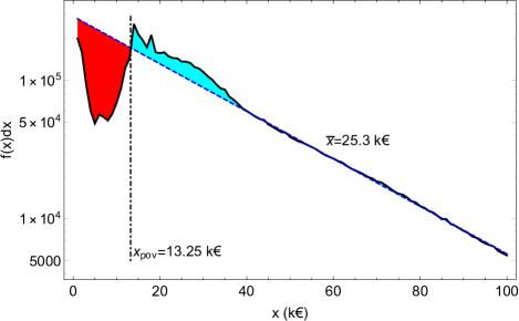
Figure 1: (color online) The (annual) income distribution in Belgium in 2014 as obtained from personal tax records taxdata , in bins of d$x=1$ k€. The distribution follows a Boltzmann law (dashed line) except for the lowest income. Redistributive taxation lifts people with an income below $x_{\textrm{pov}}$ (area shaded in dark red) above this poverty threshold (area shaded in light blue).

To illustrate the results with numbers, I use my home country of Belgium as an example, taking $x_{c}\approx 100$ k€. There were $N_{\textrm{tot}}=6.26\times 10^{6}$ people filing a non-zero income tax record in Belgium in 2014, the latest year with complete information taxdata . Of these, $N_{\textrm{cap}}=1.73\times 10^{5}$ (or 2.8% of the total) indicate an income above $x_{c}$. The remaining $N_{\textrm{lab}}=6.09\times 10^{6}$ are in the exponential regime and represent a cumulative income of $M_{\textrm{lab}}=170.6$ G€. As seen in Fig. 1, there is a strong deviation of the exponential regime for income levels below $x_{\textrm{pov}}=13.25$ k€: this is the poverty threshold. People below this threshold receive social security benefits lifting them to roughly the threshhold level and slightly above.

Estimating the amount of capital income $M_{\textrm{cap}}$ for Belgium is difficult to do based on tax forms. The reason is that not all sources of capital income need to be declared in Belgium: For instance, income from renting out apartments or offices is not declared. Piketty Piketty provides an alternative way to estimate $M_{\textrm{cap}}$ from $M_{\textrm{lab}}$. His study of the historical ratio between capital income and labor income for developed economies shows that this income has its own slow dynamics over time. Currently, the capital share of income in rich countries stands at 25-30% of national income. The dynamics of the capital/labor income ratio is slow enough such that the income distribution is close to equilibrium at any time. Taking the above-mentioned capital share of the national income into account results in an estimatenoot1 of $M_{\textrm{cap}}\approx 60$ G€.

The additive class, $x_{\textrm{pov}}<x<x_{c}$ is subject to the (normalized) Boltzmann-Gibbs distrubution

$$f_{\textrm{lab}}(x)=\frac{N_{\textrm{lab}}}{\bar{x}}\exp(-x/\bar{x}),$$ (1)

with $\bar{x}=M_{\textrm{lab}}/N_{\textrm{lab}}$ the average income in this class.

The multiplicative class is subject to the power law distribution

$$f_{\textrm{cap}}(x>x_{c})=\frac{(\gamma-1)N_{\textrm{cap}}}{x_{c}}(x/x_{c})^{-\gamma}.$$ (2)

The Pareto parameter $\gamma$ is fixed by $M_{\textrm{cap}}$ through the normalization $M_{\textrm{cap}}=\int_{x_{c}}^{\infty}{xf_{\textrm{cap}}(x)dx}$ by

$$\gamma=\frac{2M_{\textrm{cap}}-N_{\textrm{cap}}x_{c}}{M_{\textrm{cap}}-N_{\textrm{cap}}x_{c}}.$$ (3)

This restricts $\gamma>2$, since $M_{\textrm{cap}}>N_{\textrm{cap}}x_{c}$. The estimate $M_{\textrm{cap}}=60$ G€  based on Piketty’s observations corresponds to $\gamma=2.4$. This value is in agreement with the estimate of $\gamma\approx 2.5$ obtained by Silva and Yakovenko Silva2006 .

Eq. (3) can also be inverted, so that an empirical fit yielding $\gamma$ (in combination with $x_{c}$ and $N_{\textrm{cap}}$) may be used to estimate the total amount of income from capital. Detailed data for the high-income distribution is not publicly available in Belgium, and as mentioned above, exemption of some capital income sources in Belgium complicates data finding. However, for countries with an obligation to declare all capital income, Eq. 3 could be used to estimate the amount of undeclared income and hence the level of tax evasion by rentiers. A similar proposal, based on deviations from the Pareto distribution, was introduced to estimate the size of shadow banking Marsili .

III Taxing capital income

Suppose one wants to levy taxes to raise a given amount $\Delta M$ of money. For example, to bring all the poor to a minimum wage of $x_{\textrm{pov}}$, one would need

$$\Delta M = \int_{0}^{x_{c}}(x_{c}-x)f_{\textrm{lab}}(x)dx$$ (4)

$$= M_{\textrm{lab}}\left[(x_{\textrm{pov}}/\bar{x})-(1-e^{-x_{\textrm{pov}}/\bar{x}})\right].$$ (5)

Using the numbers listed above for Belgium, the topping up of all lower incomes to $x_{\textrm{pov}}$ would require 16.4 G€.

Suppose moreover that one wants to obtain the amount of $\Delta M$ by taxing capital income in such a way that the after-tax capital income distribution follows again a Pareto law. The post-tax power law distribution necessarily has a different exponent $\eta>\gamma$, given by

$$\eta=\frac{2(M_{\textrm{cap}}-\Delta{M})-N_{\textrm{cap}}x_{c}}{M_{\textrm{cap}}-\Delta{M}-N_{\textrm{cap}}x_{c}}.$$ (6)

In our Belgian example, this would mean a change from $\gamma=2.41$ to $\eta=2.66$. To describe the taxation scheme, we introduce a function $X(x)$ that gives the post-tax net income $X$ as a function of the pre-tax income $x$. The distribution of post-tax income is denoted by

$$f_{\textrm{cap}}^{\textrm{post-tax}}(X)=\frac{(\eta-1)N_{\textrm{cap}}}{x_{c}}(X/x_{c})^{-\eta}.$$ (7)

This distribution has to obey

$$f_{\textrm{cap}}^{\textrm{post-tax}}(X)dX=f_{\textrm{cap}}[x(X)]dx.$$ (8)

Substituting the Pareto distributions in the above equation yields a differential equation for X(x),

$$\frac{(\eta-1)}{x_{c}^{1-\eta}}X^{-\eta}(x)\frac{dX}{dx}=\frac{(\gamma-1)}{x_{c}^{1-\gamma}}x^{-\gamma}.$$ (9)

It solution depends on the parameter

$$\tau=\frac{\gamma-1}{\eta-1},$$ (10)

and is given by

$$X(x)=x_{c}^{1-\tau}x^{\tau}.$$ (11)

As $\tau<1$, this solution corresponds to a weighted geometric averaging between the capital income and the threshold $x_{c}$ where main income switches from additive to multiplicative. For a pre-tax income $x$ the corresponding tax rate $T(x)=(x-X)/x$ is given by

$$T(x)=1-\left(x_{c}/x\right)^{1-\tau}.$$ (12)

Figure 2: Taxation levels as a function of capital income, for different values of the parameter $\tau$, which is fixed by the amount of tax $\Delta M$ that will be levied from the total capital income $M_{\textrm{cap}}$. The tax rate is progressive and taxation starts at the income level $x_{c}$ separating the Boltzmann-type labor income distribution from the Pareto-type capital income distribution.

This represents a progressive tax rate. Taking our example $\tau=0.85$, and the resulting tax rate is shown as the full curve in Fig. 2. Whereas for a capital income of 120 k€  (slightly above the threshold when one can be called a rentier or “rich”) the tax rate is about 3%, at 200 k€  it has risen to 10%, doubling again to 20% for 500 k€.

IV Discussion and conclusions

Eqs. (6),(10) and (12) represent a simple taxation scheme that preserves the power law nature of capital income. In order to implement it, policy makers need to select a threshold $x_{c}$ of income from capital above which the tax is levied, and choose a value of $\tau$, or equivalently, an amount $\Delta M$ of money that the tax should raise. The basic idea behind preserving the power law is that this law represents a distribution in which the market is in equilibrium.

Free market proponents claim, in the first fundamental theorem of welfare economics, that a competetive market produces a (non-unique) Pareto efficient equilibrium outcome. Moreover, in this train of thought, a social planner could select the most suitable efficient outcome by lump sum transfers, according to the second fundamental theorem. In this context, the current proposal for taxation is precisely a way to organise a transfer that links one equilibrium for capital income to another.

What if one would use the same logic to labor income? Changing one Boltzmann distribution into another only requires a scale change $x\rightarrow\alpha x$ where $\alpha=1-\Delta M/M_{\textrm{lab}}$. This corresponds to a proportional tax system (a “flat tax”, such as a fixed sales tax). This is not always seen as the socially most desirable outcome as it penalizes the low-income segment of the population, who have less disposable income. In essence, the current proposal represents a flat tax on $\log(x)$, modified by the presence of a the threshold $x_{c}$. Regardless of the desirability debate, it is clear that proponents of a flat tax for labor income who base their arguments on market efficiency, should then logically advocate the current progressive tax on capital income. Another commonly encountered argument for a flat tax is its simplicity. In this respect, the proposal for a progressive capital income taxation put forward in this paper offers a scheme which, at least to a physicist, is of similar simplicity.

References

- (1) Econophysics of Wealth Distributions, ed. A. Chatterjee, S. Yarlagadda, B.K. Chakrabarti (Springer Verlag, Milan, 2005).
- (2) A. Chatterjee and B.K. Chakrabarti, Eur. Phys. J. B 60, 135 (2007).
- (3) V.M. Yakovenko and J. Barkley Rosser, Rev. Mod. Phys. 81, 1703 (2009).
- (4) B.K. Chakrabarti, A. Chakraborti, S.R. Chakravarti, and A. Chatterjee, Econophysics of Income and Wealth Disitributions (Cambridge University Press, Cambridge, 2013).
- (5) A.A. Dragulescu and V.M. Yakovenko, Eur. Phys. J. B 17, 723 (2000).
- (6) S. Ispolatov, P.L. Krapivsky, S. Redner, Eur. Phys. J. B 2, 267 (1998).
- (7) G. Willis and J. Mimkes, e-print arXiv:cond-mat/0406694
- (8) V. Pareto, Cours d’Economie Politique (ed. F. Rouge, Librairie de l’Université, Lausanne, 1897).
- (9) F. Clementi and M. Gallegati, Income Inequality Dynamics: Evidence from a Pool of Major Industrialized Countries, Talk at the International Workshop of Econophysics of Wealth Distributions, Kolkata, March 15-19, 2005. Retrieved from http://www.saha.ac.in/cmp/econophysics/abstracts.html.
- (10) T.L. Hungerford, Changes in the Distribution of Income Among Tax Filers Between 1996 and 2006: The Role of Labor Income, Capital Income, and Tax Policy, Congressional Research Service, 2011. Retrieved from http://taxprof.typepad.com/files/crs-1.pdf
- (11) M. Levy and H. Levy, Rev. Econ. Stat. 85, 709 (2003).
- (12) Y. Fujiwara, W. Souma, H. Aoyama, T. Kaizoji, and M. Aoki, Physica A 321, 598 (2003).
- (13) M. Levy and S. Solomon, Int. J. Mod. Phys. C 7, 595 (1996).
- (14) A.A. Dragulescu and V.M. Yakovenko, Physica A 299, 213 (2001).
- (15) A.A. Dragulescu and V.M. Yakovenko, Statistical mechanics of money, income, and wealth: a short survey. In Garrido, P.L., and Marro, J. (eds.), Modeling of Complex Systems: Seventh Granada Lectures, vol. 661. American Institute of Physics (AIP) Conference Proceedings. Melville, NY, AIP (2003).
- (16) A.C. Silva and V.M. Yakovenko, Europhys. Lett. 69, 304 (2005).
- (17) Data source: Algemene Directie Statistiek - Statistics Belgium, Fiscale inkomens, http://statbel.fgov.be/nl/modules/publications/statistiques/arbeidsmarkt_levensomstandigheden/Statistique_fiscale_des_revenus.jsp, retrieved on July 1st, 2017.
- (18) T. Piketty, Capital in the Twenty-First Century (translation A. Goldhammer, Harvard University Press, Cambridge, USA, 2014).
- (19) D. Fiaschi, I. Kondor, M. Marsili, V. Volpati, PLoS ONE 9, e94237 (2014).