Topological magnetoelectric pump in three dimensions

Abstract

We study the topological pump for a lattice fermion model mainly in three spatial dimensions. We first calculate the U(1) current density for the Dirac model defined in continuous space-time to review the known results as well as to introduce some technical details convenient for the calculations of the lattice model. We next investigate the U(1) current density for a lattice fermion model, a variant of the Wilson-Dirac model. The model we introduce is defined on a lattice in space but in continuous time, which is suited for the study of the topological pump. For such a model, we derive the conserved U(1) current density and calculate it directly for the $1+1$ dimensional system as well as $3+1$ dimensional system in the limit of the small lattice constant. We find that the current includes a nontrivial lattice effect characterized by the Chern number, and therefore, the pumped particle number is quantized by the topological reason. Finally we study the topological temporal pump in $3+1$ dimensions by numerical calculations. We discuss the relationship between the second Chern number and the first Chern number, the bulk-edge correspondence, and the generalized Streda formula which enables us to compute the second Chern number using the spectral asymmetry.

I Introduction

In a topological background such as a soliton or a vortex, the vacuum state of the Dirac fermion shows a nontrivial topological structure. Goldstone and Wilczek (1981); Wilczek (1987) One of famous examples in condensed matter physics is the mid-gap states of the SSH soliton,Su et al. (1979, 1980) which can be effectively described by a Dirac fermion model with a nontrivial mass term.Takayama et al. (1980) Recent discovery of topological insulators Kane and Mele (2005); Qi et al. (2008) tells us that topological states of matter are richer than we expected, Hasan and Kane (2010); Qi and Zhang (2011) and the Dirac fermion model is very convenient for the classification of symmetry classes. Schnyder et al. (2008); Ryu et al. (2010)

The topological pump in one dimensional (1D) systems has been proposed by Thouless,Thouless (1983) and experimentally observed quite recently. Nakajima et al. (2016); Lohse et al. (2016) This can also be described very simply by the Dirac fermion, as already seen in Ref. Goldstone and Wilczek (1981). The topological pump has been generalized to three dimensional (3D) systems.Qi et al. (2008) The 3D pump is unique, since it is a part of topological magneto-electric effect, Qi et al. (2008) which has close relationship with the chiral anomaly of the Dirac fermion.Wilczek (1987) Here, the pumping parameter plays a role of the axion field.Wilczek (1987) The magneto-electric response in generic systems has also been studied by developing the theory of the orbital magneto-electric polarization. Essin et al. (2009, 2010); Malashevich et al. (2010)

The chiral magnetic effect (CME), originally proposed for the quark-gluon plasma, Fukushima et al. (2008) has also been attracting much interest in condensed matter physics. In particular, the discovery of the Weyl semimetal Murakami (2007); Burkov and Balents (2011); Wan et al. (2011); Xiong et al. (2015a, b); Zhang et al. (2017) has led our interest to the observation of the chiral anomaly in a crystal through the magneto-electric response, Nielsen and Ninomiya (1983); Chen et al. (2013); Parameswaran et al. (2014) including the CME, Başar et al. (2014); Zyuzin and Burkov (2012); Jian-Hui et al. (2013); Chang and Yang (2015); Ma and Pesin (2015); Sumiyoshi and Fujimoto (2016); Alavirad and Sau (2016); O’Brien et al. (2017); Sekine and Nomura (2016); Sekine (2016) the anomalous Hall effect (AHE), Yang et al. (2011); Zyuzin and Burkov (2012); Grushin (2012); Vazifeh and Franz (2013); Goswami and Tewari (2013); Sekine and Nomura (2016); Sekine (2016) axial-magneto-electric effect, Grushin et al. (2016); Pikulin et al. (2016) and Z₂ anomaly in Dirac semimetals, Burkov and Kim (2016) etc. Thus, the chiral anomaly and its related phenomena have been one of hot topics in condensed matter physics.

In this paper, we examine mainly the topological pump in a 3D system using a lattice fermion model. In the next section II, we present the U(1) current of the Dirac fermion in continuous space-time. Here, some notations are fixed and some techniques convenient to the lattice model are given. In Sec. III.1, we introduce a Wilson-Dirac model defined on the spatial 1D or 3D lattice but in continuous time to study the topological temporal pump in Sec. IV. Throughout the paper, this model is simply referred to as Wilson-Dirac model. In Sec. III.2, we derive the conserved U(1) current density for the Wilson-Dirac model. Because of continuous time, the charge density is the same as that of the Dirac fermion, whereas the current density includes some lattice effects. Therefore, we calculate the charge density and the current density separately in Sec. III.3 and Appendix A. In Sec. III.4, we calculate the Chern numbers exactly. In particular, we show that the 3D model has nontrivial second Chern number $1$ or $-2$. It should be noted that such second Chern numbers are due to the Berry curvature of the wave function in the zero field limit. Derivation of the exact conserved current and the second Chern number for the lattice Wilson-Dirac model are one of main results of the present paper.

In Sec. IV, we restrict our discussions to the temporal 3D pump, and present some numerical results in detail. Various numerical analyses of the 3D pump which give physical interpretations of the exact results in Sec. III are another main results of the present paper. In Sec. IV.1, the number of pumped particles is explicitly derived in the case of a static and uniform magnetic field. This number is proportional to the second Chern number as well as the magnetic field and the system size.Qi et al. (2008) In 3D systems, particles are pumped toward the direction of the applied magnetic field. Qi et al. (2008) Therefore, it can also be viewed as a 1D pump. Based on the Thouless formula for the 1D pump, Thouless (1983) the number of the pumped particle is rederived, which is given by the first Chern number. Here, the first Chern number is computed using the wave function under the magnetic field. The equivalence of the two formula gives an interesting relation between two kinds of Chern numbers. We present numerical calculation of the first Chern number, and show that this relation is valid as far as the mass gap is open. The relationship between the second Chern number associated with the Berry curvature under zero magnetic field and the first Chern number associated with the Berry curvature under a finite magnetic field is one of the main results.

In Sec. IV.3, we consider the system with boundaries perpendicular to the magnetic field. Then it is possible to define the center of mass of the occupied particles along the pumped direction, which played a central role in the experimental observation of the 1D pump. Wang et al. (2013); Nakajima et al. (2016); Lohse et al. (2016) We show that the bulk-edge correspondence recently established for the 1D pump Hatsugai and Fukui (2016) is also valid for the 3D pump. Thus, from the behavior of the center of mass as the function of time, we can compute the number of the pumped particle, and hence the second Chern number.

Finally in Sec. IV.4, we give an alternative method of computing the second Chern number (and hence, the number of the pumped particles) using the generalized Streda formula.Fukui and Fujiwara (2016) This method is based on the four dimensional Hamiltonian in discrete time whose spectral asymmetry gives the chiral anomaly for the lattice fermion. Since the generalized Streda formula is the only one method of numerically computing the second Chern number for generic models, the success in reproducing the exact Chern number for the present model is of significance. In Sec. V, we give summary and discussion including outlook.

II Dirac model

The main topic of this paper is to calculate the U(1) current for the Dirac fermion on the lattice, including external scalar and pseudscalar fields which serve as nonuniform mass terms. Calculations on the lattice, however, is quite complicated, so that we first examine the Dirac fermion defined in continuous space-time, which may be of help in Sec. III.

Let us directly calculate the vector current for the model described by the Lagrangian density

$${\cal L}=\bar{\psi}\left(i\gamma^{\mu}D_{\mu}-\sigma-i\gamma_{5}\pi\right)\psi,$$ (1)

where $\mu=0,1$ with $\gamma^{0}=\sigma^{1}$, $\gamma^{1}=-i\sigma^{2}$, and $\gamma_{5}=\sigma^{3}$ for a $d=1+1$ model, whereas $\mu=0,\cdots,3$ for a $d=3+1$ model with $\gamma$ matrices defined by

$$\gamma^{0}=\begin{pmatrix}0&\bm{1}\\ \bm{1}&0\end{pmatrix},\quad\bm{\gamma}=\begin{pmatrix}0&-\bm{\sigma}\\ \bm{\sigma}&0\end{pmatrix},\quad\gamma_{5}=\begin{pmatrix}\bm{1}&0\\ 0&-\bm{1}\end{pmatrix}.$$ (2)

These satisfy $\{\gamma^{\mu},\gamma^{\nu}\}=2g^{\mu\nu}$, where $g^{\mu\nu}=\mbox{diag}(1,-1,-1,-1)$, and $\gamma_{5}=i\gamma^{0}\gamma^{1}\gamma^{2}\gamma^{3}$. The covariant derivative under a background electro-magnetic field is defined by $D_{\mu}=\partial_{\mu}-ieA_{\mu}(x)$. Note $e<0$ for electrons. We have introduced external scalar and pseudscalar fields denoted by $\sigma$ and $\pi$. This model has been studied in Ref.Goldstone and Wilczek (1981) for the fractional fermion numbers on solitons and in Ref. Sekine (2016) for the CME and AHE for an antiferromagnetic topological insulator with broken time reversal and parity symmetries. In this paper, we assume that $\sigma$ and $\pi$ depend on the coordinates $x=(t,\bm{x})$ through a single parameter $\theta(x)$ such that $\sigma(x)=m\cos\theta(x)$ and $\pi(x)=m\sin\theta(x)$. Then, we readily see that $\sigma+i\gamma_{5}\pi=me^{i\gamma_{5}\theta}$ in Eq. (1). This model is invariant not only U(1) but also axial U(1) transformations, $\psi\rightarrow e^{i\gamma_{5}\alpha}\psi$, $\bar{\psi}\rightarrow\bar{\psi}e^{i\gamma_{5}\alpha}$, and $\theta\rightarrow\theta-2\alpha$. In what follows, we calculate the U(1) vector current in the $m\rightarrow\infty$ limit.

The U(1) vector current is defined by

$$\langle j^{\mu}(x)\rangle =\langle 0|\bar{\psi}(x)\gamma^{\mu}\psi(x)|0\rangle$$

$$=-\lim_{x^{\prime}\rightarrow x}{\rm tr}\,\gamma^{\mu}\langle 0|T\psi(x)\bar{\psi}(x^{\prime})|0\rangle,$$ (3)

where the propagator is given by

$$\langle 0|T\psi(x)\bar{\psi}(x^{\prime})|0\rangle=\frac{i}{i\not{D}-me^{i\gamma_{5}\theta}+i\epsilon}\delta(x-x^{\prime}).$$ (4)

The positive infinitesimal constant $\epsilon$ will be sometimes suppressed for simplicity below. Inserting

$$\delta(x-x^{\prime})=\int\frac{d^{d}k}{(2\pi)^{d}}e^{ik(x-x^{\prime})},$$ (5)

with $kx=\omega t-\bm{k}\cdot\bm{x}$ and $d=2$ $(4)$ for a $1+1$ ($1+3$) dimensional system, we can write Eq. (3) as

$$\langle j^{\mu}(x)\rangle=\int\frac{d^{d}k}{i(2\pi)^{d}}e^{-ikx}{\rm tr}\,\gamma^{\mu}\frac{1}{i\not{D}-me^{i\gamma_{5}\theta}+i\epsilon}e^{ikx}.$$ (6)

To calculate the topological sector of the current, it is convenient to use the identity

$$\frac{1}{i\not{D}-me^{i\gamma_{5}\theta}}=(-i\not{D}-me^{-i\gamma_{5}\theta})\frac{1}{\not{D}^{2}+m^{2}+me^{i\gamma_{5}\theta}\gamma_{5}\not{\partial}\theta}.$$ (7)

In the denominator, we further have $\not{D}^{2}=D^{\mu}D_{\mu}-\frac{i\gamma^{\mu}\gamma^{\nu}}{2}eF_{\mu\nu}$, where $F_{\mu\nu}=\partial_{\mu}A_{\nu}-\partial_{\nu}A_{\mu}$ is the field strength of the background electro-magnetic field. Note also $e^{-ikx}\not{D}e^{ikx}=\not{D}+i\not{k}$. Finally, let us make a scale transformation for the momentum, $k^{\mu}\rightarrow mk^{\mu}$, and expand the propagator with respect to $1/m$. Then, Eq. (6) becomes

$$\langle j^{\mu}(x)\rangle =\int\frac{d^{d}k}{i(2\pi)^{d}}m^{d-2}{\rm tr}\,\gamma^{\mu}(-i\not{D}+m\not{k}-me^{-i\gamma_{5}\theta})\frac{1}{1-k^{2}+e^{i\gamma_{5}\theta}\gamma_{5}\not{\partial}\theta/m-\frac{i\gamma^{\rho}\gamma^{\sigma}}{2}eF_{\rho\sigma}/m^{2}+\mathcal{O}/m^{2}}$$

$$=\int\frac{d^{d}k}{i(2\pi)^{d}}\sum_{n=0}^{\infty}\frac{m^{d-1-n}}{(1-k^{2}-i\epsilon)^{n+1}}{\rm tr}\,\gamma^{\mu}\left(-i\frac{\not{D}}{m}+\not{k}-e^{-i\gamma_{5}\theta}\right)\left(-e^{i\gamma_{5}\theta}\gamma_{5}\not{\partial}\theta+\frac{i\gamma^{\rho}\gamma^{\sigma}}{2m}{eF}_{\rho\sigma}+\frac{\mathcal{O}}{m}\right)^{n},$$ (8)

where $k^{2}=\omega^{2}-\bm{k}^{2}$ and $\mathcal{O}=2ik^{\mu}D_{\mu}+D^{\mu}D_{\mu}$. The topological sector of the current is associated with the terms including $\gamma_{5}$. For the $d=1+1$ system, using (94), it turns out that the $n=1$ term in Eq. (8) survives in the $m\rightarrow\infty$ limit. Thus, we have

$$\langle j^{\mu}(x)\rangle =\int\frac{d^{2}k}{i(2\pi)^{2}}\frac{{\rm tr}\,\gamma^{\mu}\gamma_{5}\gamma^{\nu}\partial_{\nu}\theta}{(1-k^{2}-i\epsilon)^{2}}+O(m^{-1})=\frac{1}{2\pi}\epsilon^{\mu\nu}\partial_{\nu}\theta,$$ (9)

where we have used Eq. (96). For the $d=3+1$ system, using (95), we see that among terms with $\gamma_{5}$, only those included in the $n=2$ term in Eq. (8) survive,

$$\langle j^{\mu}(x)\rangle =\int\frac{d^{4}k}{i(2\pi)^{4}}\frac{m}{(1-k^{2}-i\epsilon)^{3}}{\rm tr}\,\gamma^{\mu}\cdot 2\gamma_{5}\gamma^{\nu}\partial_{\nu}\theta\frac{i\gamma^{\rho}\gamma^{\sigma}}{2m}{eF}_{\rho\sigma}+O(m^{-1})=-\frac{e}{8\pi^{2}}\epsilon^{\mu\nu\rho\sigma}(\partial_{\nu}\theta)F_{\rho\sigma}.$$ (10)

This result can be written more explicitly as

$$\rho(x)=\frac{-e}{4\pi^{2}}\nabla\theta(x)\cdot\bm{B}(x),$$

$$\bm{j}(x)=\frac{e}{4\pi^{2}}\left[\dot{\theta}(x)\bm{B}(x)+\nabla\theta(x)\times\bm{E}(x)\right].$$ (11)

Thus, we have reached the known result.Wilczek (1987); Qi et al. (2008) In the next section, we use a similar method to calculate the current for the Wilson-Dirac model.

III Wilson-Dirac model

In this section, we calculate the U(1) current density for the Wilson-Dirac model based on a similar technique demonstrated in Sec. II.

III.1 Lattice action

We consider the Wilson-Dirac HamiltonianQi et al. (2008) defined on the 1D or 3D regular lattices,

$$H=\sum_{\bm{x}}a^{d-1}\psi^{\dagger}(t,\bm{x}){\cal H}(t,\bm{x})\psi(t,\bm{x}),$$

$${\cal H}(t,\bm{x})\equiv-i\bm{\alpha}\cdot\bm{D}^{\rm L}-\beta\left(\frac{m}{a}e^{i\gamma_{5}\theta}+\frac{ba}{2}\Delta^{\rm L}\right),$$ (12)

where $a$ is the lattice constant, and $\bm{\alpha}$ and $\beta$ are given by the $\gamma$-matrices in Sec. II, $\bm{\alpha}=\beta\bm{\gamma}$ and $\beta=\gamma^{0}$. The mass is written by $m/a$, where $m$ is a dimensionless parameter. We will keep $m$ finite as $a\rightarrow 0$. This corresponds to taking $m\rightarrow\infty$ limit in the continuum theory in Sec. II. The lattice operators are introduced by

$$D_{j}^{\rm L} =\frac{1}{2}(\nabla_{j}+\nabla_{j}^{*}),\quad\Delta^{\rm L}=\frac{1}{a}\sum_{j}(\nabla_{j}-\nabla_{j}^{*}),$$ (13)

where the forward and backward covariant differences are defined by

$$\nabla_{j}\psi(t,\bm{x})=\frac{1}{a}\left[U_{j}(t,\bm{x})\psi(t,\bm{x}+a\hat{j})-\psi(t,\bm{x})\right],$$

$$\nabla_{j}^{*}\psi(t,\bm{x})=\frac{1}{a}\left[\psi(t,\bm{x})-U^{\dagger}_{j}(t,\bm{x}-a\hat{j})\psi(t,\bm{x}-a\hat{j})\right],$$ (14)

with the gauge field $U_{j}(t,\bm{x})=e^{-ieaA_{j}(t,\bm{x})}$, and $\hat{j}$ stands for the unit vector in the $j$ direction. The term associated with the Laplacian on the lattice, $\Delta^{\rm L}$, is the Wilson term originally introduced to avoid the doubling of fermions. It violates the axial U(1) symmetry and is the origin of the axial anomaly. In the condensed matter physics literature, it is known to control the topological property of the ground state. In this paper, we consider the case $b>0$. We derive the current of the lattice model in the limit $a\rightarrow 0$ in a way similar to the continuum model in Sec. II.

We treat time $t$ as continuous variable, so that the lattice action reads

$$S=\int_{-\infty}^{\infty}dt\sum_{\bm{x}}a^{d-1}\bar{\psi}(x)\left(i\not{D}^{\rm L}-\frac{m}{a}e^{i\gamma_{5}\theta}-\frac{ba}{2}\Delta^{L}\right)\psi(x),$$ (15)

where $x=(t,\bm{x})$ and the covariant derivative with respect to $t$ is the same as that in the continuum model, $D_{0}\equiv D_{0}^{\rm L}=\partial_{0}-ieA_{0}$.

The fermion propagator on the lattice is

$$\langle 0 |T\psi(x)\bar{\psi}(x^{\prime})|0\rangle$$

$$=\frac{1}{i\not{D}^{\rm L}-\frac{m}{a}e^{i\gamma_{5}\theta}-\frac{ba}{2}\Delta^{\rm L}+i\epsilon}\frac{i}{a^{d-1}}\delta(t-t^{\prime})\delta_{\bm{x},\bm{x}^{\prime}},$$ (16)

where $\epsilon$ is a positive infinitesimal constant to implement the time ordering, which will be sometimes suppressed for simplicity below. This follows from the identity

$$0 =\frac{1}{Z}\int{\cal D}\psi{\cal D\bar{\psi}}\frac{\delta}{\delta\bar{\psi}(x)}\left[e^{iS}\bar{\psi}(x^{\prime})\right]$$

$$=ia^{d-1}\left(i\not{D}^{\rm L}-\frac{m}{a}e^{i\gamma_{5}\theta}-\frac{ba}{2}\Delta^{\rm L}\right)\langle\psi(x)\bar{\psi}(x^{\prime})\rangle$$

$$\qquad+\delta(t-t^{\prime})\delta_{\bm{x},\bm{x}^{\prime}}.$$ (17)

III.2 Conserved U(1) current

The action (15) is invariant under the gauge transformation

$$\psi^{\prime}(x)=\Lambda(x)\psi(x),$$

$$\bar{\psi}^{\prime}(x)=\bar{\psi}(x)\Lambda^{\dagger}(x),$$

$$eA_{0}^{\prime}(x)=eA_{0}(x)-i\Lambda^{\dagger}(x)\partial_{0}\Lambda(x),$$

$$U^{\prime}_{j}(x)=\Lambda(x)U_{j}(x)\Lambda^{\dagger}(x+a\hat{j}).$$ (18)

For the U(1) gauge theory, the conserved current density can be obtained by considering an infinitesimal gauge transformation, $\Lambda(x)=1+i\lambda(x)$, which induces

$$\delta A_{0}(x)=\partial_{0}\lambda(x),$$

$$\delta U_{j}(x)=-ia\left(\partial_{j}\lambda(x)\right)U_{j}(x),$$

$$\delta U_{j}^{\dagger}(x-a\hat{j})=ia\left(\partial_{j}^{*}\lambda(x)\right)U_{j}^{\dagger}(x-a\hat{j}),$$ (19)

where we have introduced the forward and backward differences by

$$\partial_{j}\lambda(x)=\frac{1}{a}\left[\lambda(x+a\hat{j})-\lambda(x)\right],$$

$$\partial^{*}_{j}\lambda(x)=\frac{1}{a}\left[\lambda(x)-\lambda(x-a\hat{j})\right].$$ (20)

It is only in this subsection III.2 to use the symbols $\partial_{j}$ and $\partial_{j}^{*}$ as differences. The change of the action (15) under the infinitesimal gauge transformation reads

$$\delta S =\int dt\sum_{\bm{x}}a^{d-1}\Big{\{}\bar{\psi}(x)i\gamma^{0}\left[-ie\delta A_{0}(x)\right]\psi(x)+\frac{i}{2a}\bar{\psi}(x)\sum_{j}\gamma^{j}\left[\delta U_{j}(x)\psi(x+a\hat{j})-\delta U_{j}^{\dagger}(x-a\hat{j})\psi(x-a\hat{j})\right]$$

$$\qquad\qquad-\frac{b}{2a}\bar{\psi}(x)\sum_{j}\left[\delta U_{j}(x)\psi(x+a\hat{j})+\delta U_{j}^{\dagger}(x-a\hat{j})\psi(x-a\hat{j})\right]\Big{\}}.$$ (21)

Substituting the infinitesimal gauge transformation (19) into the above equation and using the relations $\sum_{x}\partial_{j}f(x)g(x)=-\sum_{x}f(x)\partial_{j}^{*}g(x)$, and $\partial_{j}f(x)=\partial_{j}^{*}f(x+a\hat{j})$, we have

$$\delta S =-\int dt\sum_{x}a^{d-1}\lambda(x)\Big{\{}\partial_{0}\left[\bar{\psi}(x)\gamma^{0}\psi(x)\right]+\frac{1}{2}\sum_{j}\partial_{j}^{*}\left[\bar{\psi}(x)\gamma^{j}U_{j}(x)\psi(x+a\hat{j})+\bar{\psi}(x+a\hat{j})\gamma^{j}U_{j}^{\dagger}(x)\psi(x)\right]$$

$$\qquad\qquad+\frac{ib}{2}\sum_{j}\partial_{j}^{*}\left[\bar{\psi}(x)U_{j}(x)\psi(x+a\hat{j})-\bar{\psi}(x+a\hat{j})U_{j}^{\dagger}(x)\psi(x)\right]\Big{\}}$$

$$\equiv-\int dt\sum_{\bm{x}}a^{d-1}\lambda(x)\left[\partial_{0}j^{0}(x)+\sum_{l}\partial_{l}^{*}j^{l}(x)\right],$$ (22)

where $\partial_{0}=\partial_{t}$ is the derivative with respect to $t$ and $\partial_{j}^{*}$ is the backward difference operator in Eq. (20). Thus, we reach the conserved U(1) current density

$$j^{0}(x)=\bar{\psi}(x)\gamma^{0}\psi(x),$$

$$j^{l}(x)=\bar{\psi}(x)\gamma^{l}\psi(x)+\frac{a}{2}\left[\bar{\psi}(x)\gamma^{l}\nabla_{l}\psi(x)+\bar{\psi}(x)\overleftarrow{\nabla}_{l}\gamma^{l}\psi(x)\right]+\frac{iba}{2}\left[\bar{\psi}(x)\nabla_{l}\psi(x)-\bar{\psi}(x)\overleftarrow{\nabla}_{l}\psi(x)\right],$$ (23)

where repeated $l$ in the middle term on the rhs of the second equation is not summed. We have also defined

$$a\bar{\psi}(x)\overleftarrow{\nabla}_{l}\equiv\bar{\psi}(x+a\hat{l})U^{\dagger}(x)-\bar{\psi}(x).$$ (24)

While the charge density is the same as that of the continuum theory, the current density includes lattice effects described by the differences. In what follows, we calculate the charge density and current density, separately.

III.3 Charge density in the continuum limit

The computation of the charge density $j^{0}(x)$ is much simpler than that of the current density, since we have regarded $t$ as continuous variable. Therefore, let us first start with the charge density,

$$\langle j^{0}(x)\rangle =\langle 0|\bar{\psi}(x)\gamma^{0}\psi(x)|0\rangle$$

$$=\lim_{x^{\prime}\rightarrow x}(-){\rm tr}\,\langle 0|T\gamma^{0}\psi(x)\bar{\psi}(x^{\prime})|0\rangle.$$ (25)

This can be calculated in a way similar to the continuum model. Namely, substituting the propagator (16) and inserting the plane-wave representation of the $\delta$ function, we have

$$\langle j^{0}(x)\rangle =\lim_{x^{\prime}\rightarrow x}{\rm tr}\,\gamma^{0}\frac{1}{i\not{D}^{\rm L}-\frac{m}{a}e^{i\gamma_{5}\theta}-\frac{b}{2}a\Delta^{\rm L}+i\epsilon}\frac{-i}{a^{d-1}}\delta(t-t^{\prime})\delta_{\bm{x},\bm{x}^{\prime}}$$

$$=\frac{1}{a^{d-1}}\int_{-\infty}^{\infty}\frac{d\omega}{2\pi i}\int_{-\pi}^{\pi}\frac{d^{d-1}k}{(2\pi)^{d-1}}e^{-i(\omega t-\frac{\bm{k}\cdot\bm{x}}{a})}{\rm tr}\,\gamma^{0}\frac{1}{i\not{D}^{\rm L}-\frac{m}{a}e^{i\gamma_{5}\theta}-\frac{b}{2}a\Delta^{\rm L}+i\epsilon}e^{i(\omega t-\frac{\bm{k}\cdot\bm{x}}{a})}$$

$$=\frac{1}{a^{d-1}}\int_{-\infty}^{\infty}\frac{d\omega}{2\pi i}\int\frac{d^{d-1}k}{(2\pi)^{d-1}}e^{-i\frac{kx}{a}}{\rm tr}\,\gamma^{0}\frac{1}{ia\not{D}^{\rm L}-me^{i\gamma_{5}\theta}-\frac{b}{2}a^{2}\Delta^{\rm L}+i\epsilon}e^{i\frac{kx}{a}},$$ (26)

where in the last line, we have rescaled $\omega\rightarrow\omega/a$, and $kx$ stands for the abbreviation of $\omega t-\bm{k}\cdot\bm{x}$. We will carry out the above integral in the limit $a\rightarrow 0$, implying the large mass limit $m/a\rightarrow\infty$ in the continuum model. Notice that

$$e^{-i\frac{kx}{a}}a\nabla_{j}e^{i\frac{kx}{a}}=e^{-ik_{j}}a\nabla_{j}+e^{-ik_{j}}-1,$$

$$e^{-i\frac{kx}{a}}a\nabla_{j}^{*}e^{i\frac{kx}{a}}=e^{ik_{j}}a\nabla_{j}^{*}-e^{ik_{j}}+1,$$ (27)

where $j$ denotes the spatial direction. Therefore, in the limit $a\rightarrow 0$, the difference becomes

$$e^{-i\frac{kx}{a}}aD^{\rm L}_{j}e^{i\frac{kx}{a}} =-i\sin k_{j}+\cos k_{j}aD_{j}+O(a^{2})$$

$$\equiv-is_{j}+a\widetilde{D}_{j}+O(a^{2}),$$ (28)

where $D_{j}$ in the first line is the covariant derivative in the continuum limit in Sec. II, and in the second line, the abbreviations $s_{j}$ (and $c_{j}$) mean $s_{j}\equiv\sin k_{j}$ (and $c_{j}=\cos k_{j}$), and repeated $j$ in the definition of $\widetilde{D}_{j}=c_{j}D_{j}$ is not summed. As for the time component, we simply have

$$e^{-i\frac{kx}{a}}aD^{\rm L}_{0}e^{i\frac{kx}{a}} =i\omega+aD_{0}\equiv is_{0}+a\widetilde{D}_{0}.$$ (29)

Thus, the differences $D_{\mu}^{\rm L}$ in Eqs. (28) and (29) are summarized as

$$e^{-i\frac{kx}{a}}aD^{\rm L}_{\mu}e^{i\frac{kx}{a}} =is_{\mu}+a\widetilde{D}_{\mu}+O(a^{2}),$$ (30)

where $s_{\mu}=(\omega,-s_{j})$, and $\widetilde{D}_{\mu}=c_{\mu}D_{\mu}$ (no summation over $\mu$) with $c_{\mu}=(1,c_{j})$. Likewise, the Laplacian on the lattice becomes

$$e^{-i\frac{k\cdot x}{a}}a^{2}\Delta^{\rm L}e^{i\frac{k\cdot x}{a}} =2\sum_{j=1}^{d-1}\left(\cos k_{j}-1-i\sin k_{j}aD_{j}\right)+O(a^{2})$$

$$=2\left(c_{\rm s}-ia\widetilde{D}_{\rm s}\right)+O(a^{2}),$$ (31)

where $c_{\rm s}=\sum_{j=1}^{d-1}(c_{j}-1)$ and $\widetilde{D}_{\rm s}\equiv\sum_{j=1}^{d-1}s_{j}D_{j}$. Using these, the propagator in Eq. (26) can be written as

$$e^{-i\frac{kx}{a}} \frac{1}{ia\not{D}^{L}-me^{i\gamma_{5}\theta}-\frac{b}{2}a^{2}\Delta^{L}}e^{i\frac{kx}{a}}=\frac{1}{i(i\not{s}+a\not{\widetilde{D}})-me^{i\gamma_{5}\theta}-b(c_{\rm s}-ia\widetilde{D}_{\rm s})}$$

$$=\left\{-i(i\not{s}+a\widetilde{\not{D}})-me^{-i\gamma_{5}\theta}-b(c_{\rm s}-ia\widetilde{D}_{\rm s})\right\}$$

$$\qquad\qquad\times\frac{1}{\mu^{2}-s^{2}+me^{i\gamma_{5}\theta}\gamma_{5}a\tilde{\not{\partial}}\theta-mbe^{-i\gamma_{5}\theta}\gamma_{5}a\tilde{\partial}_{\rm s}\theta-\frac{i\gamma^{\rho}\gamma^{\sigma}}{2}ea^{2}\widetilde{F}_{\rho\sigma}+ib\gamma^{\rho}ea^{2}\widetilde{F}_{\rho,{\rm s}}+\tilde{\mathcal{O}}},$$ (32)

where $s^{2}=\omega^{2}-\bm{s}^{2}$, $\tilde{\partial}_{\mu}\equiv c_{\mu}\partial_{\mu}$ (no sum over $\mu$), $\tilde{\partial}_{\rm s}=\sum_{j=1}^{d-1}s_{j}\partial_{j}$, and

$$\mu^{2}=m^{2}\sin^{2}\theta+(m\cos\theta+bc_{\rm s})^{2}.$$ (33)

We have also introduced two kinds of the field strength: First, $\widetilde{F}_{\mu\nu}\equiv c_{\mu}c_{\nu}F_{\mu\nu}$ (no sum over $\mu,\nu$) which follows from

$$[\widetilde{D}_{\mu},\widetilde{D}_{\nu}]=-ie\widetilde{F}_{\mu\nu},$$ (34)

and second, $\widetilde{F}_{\mu,{\rm s}}\equiv\sum_{j=1}^{3}c_{\mu}s_{j}F_{\mu j}$ (no sum over $\mu$) coming from

$$[\widetilde{D}_{\mu},\widetilde{D}_{\rm s}]=-ie\widetilde{F}_{\mu,{\rm s}},$$ (35)

where $F_{\mu\nu}$ is the field strength of the electro-magnetic field in the continuum model defined in Sec. II. In Eq. (32) the other operators without $\gamma$-matrices are simply denoted as $\tilde{\mathcal{O}}\equiv a^{2}\widetilde{D}^{\mu}\widetilde{D}_{\mu}+2is^{\mu}a\widetilde{D}_{\mu}-b^{2}(a^{2}\widetilde{D}_{\rm s}^{2}+2ic_{\rm s}a\widetilde{D}_{\rm s})-2imb\cos\theta a\widetilde{D}_{\rm s}$. Furthermore, we have ignored the $O(a^{2})$ terms in Eqs. (30) and (31) since they do not contribute to the charge density in the continuum limit.

For sufficiently small $a$, we can expand the denominator on the rhs of Eq. (32). The charge density (26) then can be written as

$$\langle j^{0}(x)\rangle =\frac{1}{a^{d-1}}\int_{-\infty}^{\infty}\frac{d\omega}{2\pi i}\int\frac{d^{d-1}k}{(2\pi)^{d-1}}\sum_{n=0}^{\infty}\frac{1}{(\mu^{2}-s^{2}-i\epsilon)^{n+1}}{\rm tr}\,\gamma^{0}\left(\not{s}-me^{-i\gamma_{5}\theta}-bc_{\rm s}-ia\widetilde{\not{D}}+ia\widetilde{D}_{\rm s}\right)$$

$$\times\left(-me^{i\gamma_{5}\theta}\gamma_{5}a\tilde{\not{\partial}}\theta+mbe^{-i\gamma_{5}\theta}\gamma_{5}a\tilde{\partial}_{\rm s}\theta+\frac{i\gamma^{\rho}\gamma^{\sigma}}{2}ea^{2}\widetilde{F}_{\rho\sigma}-ib\gamma^{\rho}ea^{2}\widetilde{F}_{\rho,{\rm s}}+\tilde{\mathcal{O}}\right)^{n}.$$ (36)

This equation for the lattice Wilson-Dirac fermion corresponds to Eq. (8) for the continuum Dirac fermion.

III.3.1 $d=1+1$ system

We are interested in the terms with $\gamma_{5}$ in Eq. (36) which survive in the limit $a\rightarrow 0$. Due to Eq. (94), it is enough to consider the $n=1$ term in Eq. (36).

$$\langle j^{0}(x)\rangle =\frac{1}{a}\int_{-\infty}^{\infty}\frac{d\omega}{2\pi i}\int_{-\pi}^{\pi}\frac{dk_{1}}{2\pi}\frac{{\rm tr}\,\gamma^{0}\left(\not{s}-me^{-i\gamma_{5}\theta}-bc_{\rm s}\right)(-ma\gamma_{5})\left(e^{i\gamma_{5}\theta}\tilde{\not{\partial}}\theta-be^{-i\gamma_{5}\theta}\tilde{\partial}_{\rm s}\theta\right)}{(\mu^{2}-s^{2}-i\epsilon)^{2}}.$$ (37)

It turns out that the trace in the numerator of the above equation yields

$$(-ma)\left[{\rm tr}\,\gamma_{5}\gamma^{0}\left(me^{-i\gamma_{5}\theta}+bc_{\rm s}\right)e^{i\gamma_{5}\theta}\tilde{\not{\partial}}\theta-b{\rm tr}\,\gamma_{5}\gamma^{0}\not{s}e^{-i\gamma_{5}\theta}\tilde{\partial}_{\rm s}\theta)\right]=2am\left[(m+bc_{\rm s}\cos\theta)c_{1}+b\cos\theta s_{1}^{2}\right]\epsilon^{01}\partial_{1}\theta.$$ (38)

The denominator becomes $\mu^{2}-s^{2}=\mu^{2}+\bm{s}^{2}-\omega^{2}\equiv\Omega^{2}(k_{1},\theta)-\omega^{2}$, where we have introduced a generic expression for later convenience,

$$\Omega^{2}(\bm{k},\theta) \equiv\bm{s}^{2}+\mu^{2}$$

$$=\sum_{j=1}^{d-1}s_{j}^{2}+m^{2}\sin^{2}\theta+\left[m\cos\theta+b\sum_{j=1}^{d-1}(c_{j}-1)\right]^{2}.$$ (39)

Note $d=2$ in the present 1D system. Then, using the integration over $\omega$ in Eq. (99), we finally obtain

$$\langle j^{\mu}(x)\rangle=G_{1}(\theta)\epsilon^{\mu\nu}\partial_{\nu}\theta,$$ (40)

where we have derived the $\mu=0$ charge density in this subsection, although Eq. (40) is valid for the $\mu=1$ current density, as we will show in Appendix A, and we have introduced

$$G_{d-1}(\theta)=N_{d-1}\int_{-\pi}^{\pi}d^{d-1}k\frac{\Theta(\bm{k},\theta)}{\Omega^{d+1}(\bm{k},\theta)},$$

$$\Theta(\bm{k},\theta)\equiv m\left[m+b\sum_{j=1}^{d-1}(\sec k_{j}-1)\cos\theta\right]\prod_{j=1}^{d-1}\cos k_{j},$$ (41)

with $N_{1}=1/(4\pi)$. It should be noted that $G_{d-1}(\theta)$ is independent of the electro-magnetic field, and furthermore, it depends on $x$ only through $\theta$. Thus,

$$\int_{0}^{2\pi}G_{1}(\theta)d\theta=c_{1}$$ (42)

does not depend on $x$ any longer. This is nothing but the first Chern number, which can also be computed using the wave functions of the Wilson-Dirac Hamiltonian (12). See Sec. III.4.

In the case of $\theta=\theta(x)$, Eq. (40) as well as Eq. (9) have attracted much interest as the topological number on solitons in quantum field theory.Goldstone and Wilczek (1981); Qi et al. (2008) On the other hand, when $\theta=\theta(t)$, we nowadays know that they describe the topological pump, which is of current interest. Both phenomena mentioned above are related with the anomaly in two dimensional Dirac fermions, as will be discussed in Sec. V.

III.3.2 $d=3+1$ system

We are also interested in the terms with $\gamma_{5}$ in Eq. (36) which survive in the limit $a\rightarrow 0$. Considering Eq. (95), it is enough to take the $n=2$ term in Eq. (36) into account.

$$\langle j^{0}(x)\rangle =\frac{1}{a^{3}}\int_{-\infty}^{\infty}\frac{d\omega}{2\pi i}\int\frac{d^{3}k}{(2\pi)^{3}}\frac{1}{(\mu^{2}-s^{2}-i\epsilon)^{3}}$$

$$\times{\rm tr}\,\gamma^{0}\left(\not{s}-me^{-i\gamma_{5}\theta}-bc_{\rm s}\right)\left(-me^{i\gamma_{5}\theta}\gamma_{5}a\tilde{\not{\partial}}\theta+mbe^{-i\gamma_{5}\theta}\gamma_{5}a\tilde{\partial}_{\rm s}\theta+\frac{i}{2}\gamma^{\rho}\gamma^{\sigma}ea^{2}\widetilde{F}_{\rho\sigma}-ib\gamma^{\rho}ea^{2}\widetilde{F}_{\rho,{\rm s}}\right)^{2}.$$ (43)

Among various terms in the above equation associated with the trace of the $\gamma$ matrices, the product terms between $\partial\theta$ and $\widetilde{F}$ give finite contributions, which have indeed $a^{3}$,

$$ea^{3}\Big{\{} {\rm tr}\,\gamma^{0}(-me^{-i\gamma_{5}\theta}-bc_{\rm s})(-me^{i\gamma_{5}\theta}\gamma_{5}a\tilde{\not{\partial}}\theta)(i\gamma^{\rho}\gamma^{\sigma}\widetilde{F}_{\rho\sigma})+{\rm tr}\,\gamma^{0}\not{s}mbe^{-i\gamma_{5}\theta}\gamma_{5}\tilde{\partial}_{\rm s}\theta(i\gamma^{\rho}\gamma^{\sigma}\widetilde{F}_{\rho\sigma})$$

$$+2{\rm tr}\,\gamma^{0}\not{s}(-me^{i\gamma_{5}\theta}\gamma_{5}\tilde{\not{\partial}}\theta)(-ib\gamma^{\rho}\widetilde{F}_{\rho,{\rm s}})\Big{\}}$$

$$=-mea^{3}\Big{\{}i(m+bc_{\rm s}\cos\theta){\rm tr}\,\gamma_{5}\gamma^{0}(\tilde{\not{\partial}}\theta)\gamma^{\rho}\gamma^{\sigma}\widetilde{F}_{\rho\sigma}-ib\cos\theta{\rm tr}\,\gamma_{5}\gamma^{0}\not{s}\tilde{\partial}_{\rm s}\theta\gamma^{\rho}\gamma^{\sigma}\widetilde{F}_{\rho\sigma}-2ib\cos\theta{\rm tr}\,\gamma_{5}\gamma^{0}\not{s}\tilde{\not{\partial}}\theta\gamma^{\rho}\widetilde{F}_{\rho,{\rm s}}\Big{\}}$$

$$=-4ea^{3}m\left[m+b\sum_{j=1}^{3}(\sec k_{j}-1)\cos\theta\right]\left(\prod_{j=1}^{3}\cos k_{j}\right)\epsilon^{0\nu\rho\sigma}(\partial_{\nu}\theta)F_{\rho\sigma}.$$ (44)

Thus, we finally reach

$$\langle j^{\mu}(x)\rangle=-e\frac{G_{3}(\theta)}{4\pi}\epsilon^{\mu\nu\rho\sigma}\partial_{\nu}\theta(x)F_{\rho\sigma}(x),$$ (45)

where we have derived the $\mu=0$ charge density in this subsection, although Eq. (45) is valid for the $\mu=1,2,3$ current density, as we will show in Appendix A. $G_{3}(\theta)$ is defined by Eq. (41) with $N_{3}=3/(8\pi^{2})$, which follows from Eq. (100). Note that integration of $G_{3}(\theta)$ over $\theta$ gives the second Chern number

$$\int_{0}^{2\pi}G_{3}(\theta)d\theta=c_{2}.$$ (46)

It should be stressed here that $G_{3}(\theta)$ does not depends on the electro-magnetic field. The limit $a\rightarrow 0$ implies, therefore, small field limit as well. The Chern number $c_{2}$ is alternatively calculated using the Berry curvature with respect to the eigenfunctions of the Wilson-Dirac Hamiltonian with zero fields. See Ref. Qi et al. (2008) or Fukui and Fujiwara (2016), and also Sec. III.4.

Equation (45) or its continuum version (10) show the topological magneto-electric effects, including CME and AHE. For Weyl semimetals, $\theta$ is induced by the Zeeman term violating time reversal symmetry and/or energy imbalance between the Weyl nodes breaking the inversion symmetry. In contrast, for the present Wilson-Dirac fermion, $\theta$ describes a rotation between two kinds of mass terms which keeps a finite mass gap in the spectrum. Regardless of whether the system is massless or massive, the magneto-electric effects are associated with the chiral anomaly, as will be discussed in Sec. V.

$k_{1}$	$k_{2}$	$\qquad\xi_{3}\Omega\qquad$	$\Theta(k_{1},\theta)$
$0$	$0$	$m$	$m^{2}$
$\pi$	$0$	$m-2b$	$-m(m-2b)$
$0$	$\pi$	$-m$	$m^{2}$
$\pi$	$\pi$	$-m-2b$	$-m(m+2b)$

Table 1: List of $\xi_{3}\Omega=m\cos k_{2}+b(\cos k_{1}-1)$ and $\Theta(k_{1},\theta)=m[m+b(\sec k_{1}-1)\cos k_{2}]\cos k_{1}$ at $k_{\mu}=0$ or $\pi$.

III.4 Chern numbers

For the study of the temporal pump in the next section IV, we need an explicit value of the Chern number. Therefore, we calculate the first and second Chern numbers in Eqs. (42) and (46). Fortunately, the Wilson-Dirac model is so simple that one can calculate the second Chern number exactly.

III.4.1 First Chern number

We can regard $k_{1}$ and $k_{2}\equiv\theta$ as the coordinates of a two-dimensional torus T². A mapping $f$ from T² to S² can be defined by

$$\xi_{1}=\frac{\sin k_{1}}{\Omega(k_{1},\theta)},\quad\xi_{2}=\frac{m\sin\theta}{\Omega(k_{1},\theta)},$$

$$\xi_{3}=\frac{m\cos\theta+b(\cos k_{1}-1)}{\Omega(k_{1},\theta)},$$ (47)

where $\Omega(k_{1},\theta)$ is given by Eq. (39) for $d=2$. It is known that the Chern number is the degree of the mapping which can be computed by

$$\mbox{deg }f=\frac{1}{\mbox{Vol(S}^{2})}\int\frac{1}{2!}\epsilon^{\alpha\beta\gamma}\xi_{\alpha}d\xi_{\beta}d\xi_{\gamma},$$ (48)

where $\mbox{Vol(S}^{2})=4\pi$ and $d\xi_{\alpha}$ is the coordinate differential 1-form. Indeed, it is not difficult to rewrite Eq. (48) by $k_{\mu}$ ($\mu=1,2$) to show $\mbox{deg\>}f=c_{1}$, where $c_{1}$ is given by the lhs of Eq. (42) with $G_{1}(\theta)$ in Eq. (41).

It is readily seen that only the points $k_{\mu}=0$ or $\pi$ on T² are mapped to $\xi_{\pm}=(0,0,\pm 1)$ on S². The degree of the mapping $f$ is then given by

$$\mbox{deg }f= \sum_{k\in f^{-1}(\xi_{+})}\mbox{sgn}\left[\Theta(k_{1},\theta)\right],$$ (49)

where $\Theta(k_{1},\theta)$ is defined in Eq. (41) for $d=2$. From Table 1, we can read the coordinates $k_{\mu}$ mapped to $\xi_{+}$ with its degree of mapping (or winding number) $\pm 1$. For example, when $0<m<2b$, only $(0,0)$ is mapped to $\xi_{+}$ with a positive winding number $m^{2}>0$, whereas others $(0,\pi)$, $(\pi,0)$, and $(\pi,\pi)$ are mapped to $\xi_{-}$. Thus, we find $c_{1}=1$ in this case. The other cases are likewise. Thus, Table 1 leads to

$$\mbox{deg }f=c_{1}=\left\{\begin{array}[]{rl}+1&(0<|m|<2b)\\ 0&(2b<|m|)\end{array}\right..$$ (52)

($k_{1}$, $k_{2}$, $k_{3}$)	$k_{4}$	$\qquad\xi_{5}\Omega\qquad$	$\Theta(\bm{k},\theta)$
no $\pi$	$0$	$m$	$m^{2}$
one $\pi$	$0$	$m-2b$	$-m(m-2b)$
two $\pi$	$0$	$m-4b$	$m(m-4b)$
three $\pi$	$0$	$m-6b$	$-m(m-6b)$
no $\pi$	$\pi$	$-m$	$m^{2}$
one $\pi$	$\pi$	$-m-2b$	$-m(m+2b)$
two $\pi$	$\pi$	$-m-4b$	$m(m+4b)$
three $\pi$	$\pi$	$-m-6b$	$-m(m+6b)$

Table 2: List of $\xi_{5}\Omega=m\cos k_{4}+b\sum_{j}^{3}(\cos k_{j}-1)$ and $\Theta(\bm{k},\theta)=m[m+b\sum_{j}^{3}(\sec k_{j}-1)\cos k_{4}]\prod_{j}^{3}\cos k_{j}$ at $k_{\mu}=0$ or $\pi$. “no $\pi$” in the first column means all $k_{\mu}=0$, whereas “one $\pi$” means that one of $k_{\mu}=\pi$ and others are $0$, and so on.

III.4.2 Second Chern number

The second Chern number can be obtained by extending the computation of the first Chern number for the S² to S⁴. Let us introduce $\xi_{\mu}$ ($\mu=1,\cdots,5$) by

$$\xi_{j}=\frac{\sin k_{j}}{\Omega(\bm{k},\theta)},\quad(j=1,2,3),\quad\xi_{4}=\frac{m\sin\theta}{\Omega(\bm{k},\theta)},$$

$$\xi_{5}=\frac{m\cos\theta+b\sum_{l=1}^{3}(\cos k_{l}-1)}{\Omega(\bm{k},\theta)},$$ (53)

where $\Omega(\bm{k},\theta)$ is defined in Eq. (39) for $d=4$. These define a mapping $f$ from T⁴ spanned by $(k_{1},k_{2},k_{3},\theta\equiv k_{4})$ to S⁴ spanned by $\xi_{\mu}$ satisfying $\xi_{\mu}^{2}=1$. The Chern number is the degree of the mapping given by

$$\mbox{deg }f=\frac{1}{\mbox{Vol(S}^{4})}\int\frac{1}{4!}\epsilon^{\alpha\beta\gamma\delta\epsilon}\xi_{\alpha}d\xi_{\beta}d\xi_{\gamma}d\xi_{\delta}d\xi_{\epsilon},$$ (54)

where Vol(S⁴)$=8\pi^{2}/3$. It is straightforward to rewrite Eq. (54) by $k_{j}$ and $\theta$ to show $\mbox{deg }f=c_{2}$, where $c_{2}$ is given by the lhs of Eq. (46) with $G_{3}(\theta)$ in Eq. (41). It is readily seen that the points $k_{\mu}=0$ or $\pi$ on T⁴ are mapped to $\xi_{\pm}=(0,0,0,0,\pm 1)$ on S⁴. The degree of the mapping $f$ is then given by

$$\mbox{deg }f= \sum_{k\in f^{-1}(\xi_{+})}\mbox{sgn}\left[\Theta(\bm{k},\theta)\right],$$ (55)

where $\Theta(\bm{k},\theta)$ is defined in Eq. (41) for $d=4$. Thus, the second Chern number can be obtained from Table 2 in the similar way to the first Chern number:

$$\mbox{deg }f=c_{2}=\left\{\begin{array}[]{rl}+1&(0<|m|<2b)\\ -2&(2b<|m|<4b)\\ +1&(4b<|m|<6b)\\ 0&(6b<|m|)\\ \end{array}\right..$$ (60)

IV Magneto-electric pump

In Secs. III.3 and A, we have established the U(1) current (45) in the 3D Wilson-Dirac model. This result is obtained in the limit $a\rightarrow 0$. It also implies that the result is valid only in a weak field limit. On the other hand, the pump is topological so that the result may be valid as long as the mass gap is open. To check this point, we study the pump by numerical calculations. In this section, we restrict our discussions to the 3D temporal particle pump.

IV.1 3D pump

Assume that the electro-magnetic field is static, and consider the case in which $\theta$ depends only on $t$, $\theta=\theta(t)$ with a period $T$, $\theta(t+T)=\theta(t)$. When $1/T\ll m$, we can regard the process of changing $t$ as an adiabatic process. Then, integration of Eq. (45) over $t$ in one period yields the pumped particle density

$$\bm{q}(x)=e\frac{c_{2}}{2\pi}\bm{B}(x),$$ (61)

where $c_{2}$ is the second Chern number defined in Eq. (46) and explicitly given by (60). We have stressed there that the second Chern number (46) is that of the Wilson-Dirac model in zero field limit. Namely, the Chern number can be computed directly using the eigenfunctions of the Hamiltonian without the magnetic field.

Without loss of generality, we assume the magnetic field in the $z$ direction, $(0,0,B)$. The total pumped particle number $Q^{z}$ can be defined by integrating over the $xy$ surface,

$$Q^{z}=ec_{2}\frac{\Phi}{2\pi},$$ (62)

where $\Phi$ is the total flux penetrating the surface of an area under consideration. This integration can be simply carried out, since $c_{2}$ is independent of $B$, as stressed already. For numerical computations, we further consider a simpler case where the magnetic field $B$ is uniform, and system is periodic in $xy$ surface whose size in the $x$ ($y$) direction is $N_{x}$ ($N_{y}$). Then, $\Phi=Ba^{2}N_{x}N_{y}$, and the flux per plaquette should be rational

$$|e|\phi=|e|Ba^{2}=\frac{2\pi p}{q}\equiv\phi_{0},$$ (63)

where $p$ and $q(>0)$ are integers describing a rational magnetic flux per plaquette. Hofstadter (1976); Thouless et al. (1982); Kohmoto (1985) Thus, it turns out that the total pumped particle number $Q^{z}$ is given by

$$Q^{z}=\mbox{sgn(}e)c_{2}\frac{Ba^{2}N_{x}N_{y}}{2\pi}=\mbox{sgn(}e)c_{2}\frac{p}{q}N_{x}N_{y}.$$ (64)

The elementary pump is due to a nonzero second Chern number, and $pN_{x}N_{y}/q$ can be considered as the geometrical multiplicity of pumped particles associated with the magnetic flux.

IV.2 3D pump as a set of 1D pump

The magneto-electric pump discussed so far has deep relationship with the chiral anomaly, so that the $3+1$ dimensionality plays a crucial role. However, the pumping itself is toward one direction of the applied magnetic field, and hence, it can also be viewed as a 1D pump. In this section, we derive the pumped particle number by the Thouless formula for the 1D pump.Thouless (1983); Xiao et al. (2010)

Consider the snapshot (for a fixed $t$, i.e., fixed $\theta$) many-body ground state eigenfunction obeying $H|\Psi_{n}\rangle=E_{n}|\Psi_{n}\rangle$. We assume that $|\Psi_{0}\rangle$ is the ground state and have a spectral gap $E_{n}(t)-E_{0}(t)>0$ at any time during the pump. Then, the ground state $|G\rangle$ which satisfies the time-dependent Schrödinger equation at the first order of $\hbar$ is given by

$$|G\rangle=e^{-\frac{i}{\hbar}\int^{t}E_{0}dt}\left(|\Psi_{0}\rangle+i\hbar\sum_{n\neq 0}\frac{|\Psi_{n}\rangle\langle\Psi_{n}|\dot{\Psi}_{0}\rangle}{E_{n}-E_{0}}\right).$$ (65)

For non-interacting case, it is enough to consider the single particle states. Let ${\cal H}(\theta,\bm{k};\bm{B})$ be the Fourier-transformed Hamiltonian given by Eq. (12), and let $\psi(\theta,\bm{k};\bm{B})$ be the ground state (i.e., negative energy) multiplet wave functions of single-particle states satisfying

$${\cal H}(\theta,\bm{k};\bm{B})\psi(\theta,\bm{k};\bm{B})=\psi(\theta,\bm{k};\bm{B}){\cal E}(\theta,\bm{k};\bm{B}),$$ (66)

where ${\cal E}(\theta,\bm{k},\bm{B})$ is the diagonal matrix of the energy eigenvalues.

Let us now consider the case where uniform magnetic field is applied in the $z$ direction, as studied in Sec. IV.1. Regarding $k_{x}$ and $k_{y}$ as parameters, the current toward the $z$ direction, $J^{z}$, with respect to the state Eq. (65) is given by Thouless (1983)

$$\langle J^{z}\rangle=\int_{0}^{2\pi}\frac{dk_{z}}{2\pi i}f(\theta,k_{z};k_{x},k_{y},B),$$ (67)

where $f(\theta,k_{z};k_{x},k_{y},B)\equiv\partial_{k_{z}}\psi^{\dagger}\partial_{\theta}\psi-\partial_{\theta}\psi^{\dagger}\partial_{k_{z}}\psi$ is the Berry curvature with respect to $\theta$ and $k_{z}$ with fixed $k_{x}$ and $k_{y}$. Integrating $\langle J^{z}\rangle$ with respect to $t$ in one period as well as with respect to $k_{x}$ and $k_{y}$, we obtain the total number of pumped particle,

$$Q^{z}=\sum_{k_{x},k_{y}}c_{1}(B),$$ (68)

where

$$c_{1}(B)=\frac{1}{2\pi i}\int_{0}^{2\pi}d\theta\int_{0}^{2\pi}dk_{z}f(\theta,k_{z};k_{x},k_{y},B),$$ (69)

is the first Chern number on the section specified by fixed $k_{x},k_{y}$. However, it should be noted that the Chern number $c_{1}(B)$ does depend on the applied magnetic field, but does not depend on $k_{x}$ ($\tilde{k}_{x}$) and $k_{y}$, provided that the mass gap always opens.

When we compute the eigenfunctions in the Landau gauge $U_{j}(t,\bm{x})=e^{-ieaA_{j}(t,\bm{x})}$ with

$$e\bm{A}(\bm{x})=(0,\mbox{sgn(}e)\phi\frac{x}{a},0),$$ (70)

we can take the $q$ sites in the $x$-direction as a unit cell, and therefore, we set $N_{x}=q\tilde{N}_{x}$ for the periodic boundary condition. In this case, $k_{y}=2\pi n_{y}/N_{y}$ with $n_{y}=1,\cdots,N_{y}$ , whereas $\tilde{k}_{x}=2\pi n_{x}/\widetilde{N}_{x}$ with $n_{x}=1,\cdots,\widetilde{N}_{x}$. It follows from Eq. (68) and from the fact that $c_{1}(B)$ is independent of $k_{x}$ and $k_{y}$ that

$$Q^{z}=c_{1}(B,\mbox{sgn}(e))\tilde{N}_{x}N_{y},$$ (71)

where in Eq. (68) $k_{x}$ is replaced by $\tilde{k}_{x}$, and the dependence of $c_{1}$ on the sign of the charge $e$ through Eq. (70) has been explicitly denoted. Comparing Eq. (64), we have a simple relationship between the second Chern number $c_{2}$ in the zero magnetic field and $c_{1}$ in the magnetic field $B$,

$$c_{1}(B,\mbox{sgn}(e))=\mbox{sgn}(e)c_{2}p,$$ (72)

where $p$ is given by Eq. (63). This relation may be useful for computing the second Chern number, since the numerical method of computing the first Chern number has already been established.Fukui et al. (2005)

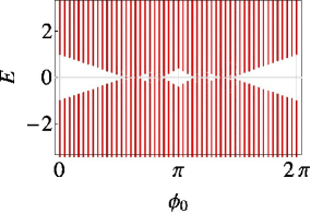
Figure 1: The Hofstadter butterfly diagrams for fixed $\theta=0$ and for $m=b$ (upper) and $m=3b$ (lower). We set $q=50$, and the system size is $\widetilde{N}_{x}=1$ and $N_{y}=N_{z}=50(=q)$.

$m=b$						$m=3b$
$\frac{p}{q}$	$c_{1}$	$\frac{p}{q}$	$c_{1}$	$\frac{p}{q}$	$c_{1}$	$\frac{p}{q}$	$c_{1}$	$\frac{p}{q}$	$c_{1}$	$\frac{p}{q}$	$c_{1}$
$\frac{1}{20}$	1					$\frac{1}{20}$	$-2$
$\frac{2}{20}$	2	$\frac{1}{10}$	1			$\frac{2}{20}$	$-4$	$\frac{1}{10}$	$-2$
$\frac{3}{20}$	3					$\frac{3}{20}$	$-6$
$\frac{4}{20}$	4	$\frac{2}{10}$	2	$\frac{1}{5}$	1	$\frac{4}{20}$	$-8$	$\frac{2}{10}$	$-4$	$\frac{1}{5}$	$-2$

Table 3: The (section) first Chern number (69) computed on the discretized $(\theta,k_{z})$ Brillouin zone Fukui et al. (2005) in the case $e<0$ for several $\frac{p}{q}=\frac{\phi_{0}}{2\pi}$.

We show in Table 3 the list of the section Chern number $c_{1}(B)$ in (69) for various $\phi_{0}$, and in Fig. 1 the corresponding Hofstadter butterfly diagrams.Hofstadter (1976) The Hofstadter diagrams tell that the mass gap at $\phi_{0}=0$ becomes smaller as a function of $\phi_{0}$, and eventually closed around $\phi_{0}\sim\pi/2$ for both cases $m=b$ and $m=3b$. Thus, it turns out from the Table 3 that the relationship (72) is indeed valid as long as the mass gap is finite. This implies the absence of the higher order corrections for the chiral anomaly. Adler and Bardeen (1969)

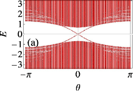
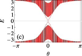
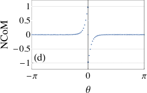
Figure 2: Upper two figures show the spectra as the function of $\theta$ of the Wilson-Dirac model for electrons ($e<0$) with top and bottom surfaces of width $N_{z}=20$ under $p/q=1/10$ magnetic flux per plaquette. Lower two figures show the normalized center of mass defined by $p_{z}(\theta)$. (a) and (b) are for the mass $m=b$ and (c) and (d) are for the mass $m=3b$. The discontinuities are (b) $p_{z}(+0)-p_{z}(-0)=0.981$ and (d) $-1.938$, which suggest that $c_{2}=1$ and $-2$.

IV.3 Bulk-edge correspondence

So far we have discussed the topological property of the bulk system. In this subsection, we discussed the surface states of the 3D topological pump, considering a system with boundaries. In Ref.Hatsugai and Fukui (2016), the bulk-edge correspondence in the 1D Thouless pump has been discussed. Consider the system with boundaries. Then one can define the center of mass of the occupied particles. Wang et al. (2013) It has been shown that the change of the center of mass is just the number of pumped particle. Wang et al. (2013) Consider here a system coupled with a particle reservoir. Then, the center of mass as a function of time shows discontinuity due to sudden change of the ground state when the chemical potential crosses the edge states.Hatsugai and Fukui (2016) After one period, the center of mass returns to the initial value. This implies that the amount of pumped particles in the bulk are compensated by these discontinuities. Thus, from the discontinuities, one can know the number of the pumped particle.Hatsugai and Fukui (2016)

Consider the Wilson-Dirac Hamiltonian with bottom and top surfaces, labeled by $j_{z}=0$ and $j_{z}=N_{z}$, respectively, perpendicular to the $z$ axis. Let $\psi^{n}(\theta,\tilde{k}_{x},k_{y};B)$ be the $n$th normalized eigenfunction of the Hamiltonian with the boundaries ${\cal H}(\theta,\tilde{k}_{x},k_{y};B)$, where we have assumed the Landau gauge in Sec. IV.2. Then, we can define the normalized center of mass of the ground state along the $z$ axis as

$$p_{z}(\theta)=\frac{1}{p\widetilde{N}_{x}N_{y}}\sum_{n~{}{\rm occ.}}\sum_{\tilde{k}_{x},k_{y}}\sum_{j_{z}=0}^{N_{z}}\left(\frac{j_{z}}{N_{z}}-\frac{1}{2}\right)|\psi_{j_{z}}^{n}(\theta,\tilde{k}_{x}.k_{y})|^{2},$$ (73)

where the normalization factor is due to the multiplicity associated with the total flux in Eq. (64). It follows from Eq. (64) that the normalized center of mass gives the second Chern number

$$c_{2}=-\mbox{sgn}(e)\left[\mbox{ sum of discontinuities of }p_{z}(\theta)\right].$$ (74)

In Fig. 2, we show the spectral flow as a function of $\theta$ and the normalized center of mass $p_{z}(\theta)$. In both cases in Fig. 2, the structure of the vacuum (negative energy states) changes at $\theta=0$, and shows the discontinuity in the center of mass, from which the second Chern number can be obtained. The result is consistent with Eq. (60).

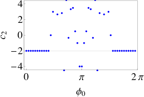
Figure 3: Upper figure shows the Hofstadter diagram of the Hamiltonian (76) as a function of the magnetic flux per plaquette (63). The parameters are $q=50$, $N_{y}=N_{z}=6$, $\tilde{q}=6$, and $\tilde{p}=1$ is fixed, whereas $p$ is changed by $\Delta p=1$. The model parameter is $m=3b$. Lower figure shows the difference of the number of the negative energy states defined in the rhs of Eq. (80).

IV.4 Generalized Streda formula

For reference, we here present a method of computing the second Chern number based on the generalized Streda formula.Fukui and Fujiwara (2016) Without an electro-magnetic field, the Wilson-Dirac Hamiltonian (12) in the momentum space reads

$${\cal H}(k)= \Gamma^{j}\sin k_{j}+m\Gamma^{4}\sin k_{4}$$

$$-\Gamma_{5}\left[m\cos k_{4}+b\sum_{j=1}^{3}(\cos k_{j}-1)\right],$$ (75)

where we have introduced $k_{4}=\theta$, and new hermitian $\Gamma$ matrices $\Gamma^{j}=\alpha^{j}$ ($j=1,2,3$), $\Gamma^{4}=-i\beta\gamma_{5}$, and $\Gamma^{5}=\beta$, with $\{\Gamma^{\mu},\Gamma^{\nu}\}=2\delta^{\mu\nu}$. Now let us regard $k_{4}$ as the frequency of discrete imaginary time. Then, we can reconstruct an equivalent lattice fermion such that

$${\cal H}= \Gamma^{j}D_{j}^{\rm L}+m\Gamma^{4}D_{4}^{\rm L}-\Gamma^{5}\left[\frac{m}{2}(\Delta_{4}^{\rm L}+2)+\frac{ba}{2}\Delta^{\rm L}\right],$$ (76)

where $D_{4}^{\rm L}\equiv(\nabla_{4}+\nabla_{4}^{*})/2$ and $\Delta_{4}^{\rm L}=(\nabla_{4}-\nabla_{4}^{*})/a$ are defined for the new coordinate $x^{4}$ in the same way as Eqs. (13) and (14).

Using this four dimensional Hamiltonian, one can define the overlap Dirac operator, Neuberger (1998a, b) which obeys the Ginsparg-Wilson relation. Ginsparg and Wilson (1982) This enables us to define the chiral anomaly on the lattice. Lüscher (1998); Kikukawa and Yamada (1999); Suzuki (1999) Taking the continuum limit, it indeed reproduces the chiral anomaly in arbitrary dimensions with a nontrivial Chern number as a coefficient.Fujiwara et al. (2002) It has been shown that the chiral anomaly thus obtained is given by the spectral asymmetry of the above Hamiltonian, and hence one can compute the second Chern number from the spectral flow of the Hamiltonian. Fukui and Fujiwara (2016) This is referred to as the generalized Streda formula. In what follows, we use $N_{-}$ rather than the spectral asymmetry $\eta=(N_{+}-N_{-})/2$, where $N_{\pm}$ is the number of positive and negative energy states.

Consider the system which includes a static and uniform magnetic field in the $x^{3}=z$ direction, as studied in Secs. IV.1, IV.2, and IV.3, and introduce a fictitious electric field associated with the imaginary time $x^{4}$ direction. As shown in Ref. Fukui and Fujiwara (2016), the density of occupied (negative energy) states

$$n_{-}=\frac{1}{2V}{\rm Tr}\left(1-\frac{{\cal H}}{\sqrt{\cal H}^{2}}\right)=\frac{N_{-}}{V}$$ (77)

of the Hamiltonian (76) as a function of the magnetic field yields the second Chern number,

$$\frac{\partial n_{-}}{\partial(\bm{B}\cdot\bm{E})}=-\frac{c_{2}}{(2\pi)^{2}},$$ (78)

where $\bm{E}$ is the fictitious electric field. To be concrete, assume that the magnetic field is included in the Landau gauge in Sec. IV.2. The fictitious electric field is also included in the $z$ direction such that

$$e\bm{A}(\bm{x})=(0,\mbox{sgn(}e)\phi\frac{x}{a},\mbox{sgn(}e)\tilde{\phi}\frac{x^{4}}{a}),$$ (79)

where $\tilde{\phi}=2\pi\tilde{p}/\tilde{q}$, gives the fictitious electric field $(0,0,E)$ such that $E=-\partial A_{z}/\partial x^{4}=-\mbox{sgn}(e)\tilde{\phi}/a^{2}$. For numerical calculations, we set the system size as $q$, $N_{y}$, $N_{z}$, and $\tilde{q}$ sites for $x$, $y$, $z$, and $x^{4}$ directions, respectively, with periodic boundary conditions imposed in all directions. Then, the volume of the system is $V=qN_{y}N_{z}\tilde{q}a^{4}$, and therefore,

$$c_{2}=-(2\pi)^{2}\frac{\Delta N_{-}}{qN_{y}N_{z}\tilde{q}a^{4}\Delta(BE)}=\frac{\Delta N_{-}}{N_{y}N_{z}\tilde{p}\Delta p},$$ (80)

where $\Delta p=1$, and we have assumed that the electric field is fixed. In Fig. 3, we show the spectrum as a function $\phi_{0}$, and corresponding difference of the density of the occupied states. This figure tells that the the second Chern number is $c_{2}=-2$, consistent with the previous results. In passing, we mention that in the case $m=b$, we can also reproduce $c_{2}=1$ in the same manner.

The Hofstadter diagram in Fig. 3 is different from that in Fig. 1, since the former includes a finite fictitious electric field. In other words, such a difference enables us to compute the second Chern number. Without the fictitious electric field, the anomaly is trivially vanishing.

V Summary and discussion

In summary, we studied mainly the 3D topological pump analytically and numerically in detail in this paper. We introduced a variant of the Wilson-Dirac model defined on the spatial lattice but in continuous time, including two kinds of mass terms depending generically on $\bm{x}$ as well as $t$. We derived the conserved current density on the lattice and calculate it in the continuum limit, or in other words in the small field limit. For the temporal pump, the result was checked by numerical calculations from various methods as follows.

Firstly, the 3D pump governed by the second Chern number (62) or (64) can be viewed as a set of 1D pump described by the first Chern number (68) or (71). It should be noted that the latter description is valid even in a strong magnetic field as long as the mass gap is open. Both results lead to the relationship between two Chern numbers (72). We showed by the numerical calculation of the first Chern number using the Berry curvature of the wave functions that Eq. (72) is valid in a strong magnetic field regime up to the gap closing point. It would be an interesting problem to ask whether the relationship (72) is restricted only to the present system or more applicable to other cases. Since the second Chern number is generically due to non-Abelian Berry curvature, its numerical calculation is very hard, and therefore, a simple relationship like (72) is quite helpful.

Secondly, as the Chern number description of the number of the pumped particles is for the bulk system, the bulk-edge correspondence enables us to observe the 3D pump as the flow of the surface states. We showed that the bulk-edge correspondence established in a 1D pump Hatsugai and Fukui (2016) can be applied to the present 3D system, and discontinuities of the center of mass of the occupied particles, which are the contribution from the surface states, reproduces the correct number of the pumped particles. The center of mass is one of important observables for the topological pump: Wang et al. (2013) Indeed, in the recent experiments of the 1D pump, Nakajima et al. (2016); Lohse et al. (2016) the center of mass played a central role. Thus, it would be expected that 3D pump can be detected experimentally using the center of mass of the occupied particles. This would also imply the experimental observation of the chiral anomaly.

In passing, we would like to add a comment on the effect of interactions. So far we have discussed the bulk-edge correspondence for a particle pump of a noninteracting system by observing the discontinuities of the center of mass of the ground state in contact with a particle reservoir. Since the present pumping is of topological origin, small interactions cannot change the quantized discontinuities of the center of mass. On the other hand, for systems with strong interactions, fractional pumping have been proposed for 1D systems with degenerate ground states. Zeng et al. (2016); Li and Fleischhauer (2017); Taddia et al. (2017) In such cases, the discontinuities of the center of mass is not obvious, but if we introduce a particle reservoir also for such systems and consider the ground states with different number of particles, we could discuss the discontinuities for the degenerate ground states. This is because of the universality of the bulk-edge correspondence: The bulk topological properties should be closely related with the edge states also for interacting systems.

Thirdly, we applied the generalized Streda formula, which is based on the chiral anomaly of the Dirac fermion, to compute the second Chern number. Let us here mention the anomaly of the present system. The current (45) may be derived from the effective action, as has been done in Ref. Qi et al. (2008). Although we did not directly calculate the effective action, we can derive it from the expressions of the current (40) and (45) as follows: Let $\Gamma_{\rm eff}[\theta,A]$ be the effective action defined by

$$i\Gamma_{\rm eff}[\theta,A]=\ln{\rm Det}\left[(i\not{D}-me^{i\gamma_{5}\theta})/(i\not{D}-m)\right].$$ (81)

Then, the current can be obtained by

$$\langle j^{\mu}(x)\rangle=\frac{1}{e}\frac{\delta\Gamma_{\rm eff}[\theta,A]}{\delta A_{\mu}(x)},$$ (82)

from which we have for $d=1+1$ system

$$\Gamma_{\rm eff}[\theta,A]=\frac{e}{2}\int d^{2}x\epsilon^{\mu\nu}P_{1}(\theta)F_{\mu\nu},$$ (83)

and for $d=3+1$ system

$$\Gamma_{\rm eff}[\theta,A]=-\frac{e^{2}}{16\pi}\int d^{4}x\epsilon^{\mu\nu\rho\sigma}P_{3}(\theta)F_{\mu\nu}F_{\rho\sigma},$$ (84)

where the charge polarization ($d=1+1$) or the magneto-electric polarization ($d=3+1$), $P_{d-1}(\theta)$, is defined by Qi et al. (2008)

$$P_{d-1}(\theta)=\int_{0}^{\theta}d\theta G_{d-1}(\theta).$$ (85)

For $\theta=2\pi$, the effective action gives the chiral anomaly. On the other hand, in Sec. IV.4 in this paper, we demonstrated the manifestation of the anomaly based on a related method developed in Ref. Fukui and Fujiwara (2016). Namely, we calculated the second Chern number from spectral asymmetry of the four dimensional Hamiltonian with an electric field as well as a magnetic field. As shown in Ref. Fukui and Fujiwara (2016), the spectral asymmetry gives the chiral anomaly of the overlap Dirac operator Neuberger (1998a, b) obeying the Ginsparg-Wilson relation. It may be usually natural to use the Wilson-Dirac Hamiltonian to construct the overlap operator $D=\frac{1}{a}\left(1-\gamma_{5}\frac{\cal H}{\sqrt{{\cal H}^{2}}}\right)$. However, for any gapped Hamiltonian, the overlap operator obeys the Ginsparg-Wilson relation.Ginsparg and Wilson (1982) Thus, it would be an interesting future problem to seek the possible Hamiltonian for the overlap operator.

Finally, we would like to add a comment on recent observations concerning the four dimensional (4D) topological pump. In Refs. Zilberberg et al. (2017); Lohse et al. (2017), the well-known two dimensional (2D) (or $d=1+1$) topological pump models such as the Harper pump model Hatsugai and Fukui (2016) or Rice-Mele model Rice and Mele (1982); Xiao et al. (2010) $H(k,t)$ are extended to a 4D model considering the direct sum, $H(k_{1},t)+H^{\prime}(k_{2},s)$. This allows a simple relationship between the second Chern number that governs the topological properties of a 4D system and the first Chern number of each 2D (or $d=1+1$) subsystem. In spite of some weak couplings between two subsystems in the experimental setup, the expected second Chern number has been observed indeed. However, if the couplings become larger, the topological change may be expected, which is an interesting future issue to explore. To this end, we note that for the lowest non-degenerate band studied in Refs. Zilberberg et al. (2017); Lohse et al. (2017), the second Chern number associated with the U(1) Berry curvature can be computed directly on the lattice. Lüscher (1999a, b); Fujiwara et al. (2002) Also it may be interesting to develop several numerical techniques studied in Sec. IV for these non-Dirac systems, or to apply the techniques of the entanglement Chern number, which can separate the Chern number into those of subsystems.Fukui and Hatsugai (2014); Araki et al. (2017).

Appendix A Current density in the continuum limit

In this Appendix, we calculate the current density given by Eq. (23). It is similar to the charge density, but it includes the lattice corrections. From Eq. (23), we need to calculate

$$\langle j^{l}(x)\rangle =-\lim_{x^{\prime}\rightarrow x}{\rm tr}\,\langle 0|T\Big{\{}\gamma^{l}\psi(x)\bar{\psi}(x^{\prime})+\frac{a}{2}\gamma^{l}\left[\nabla_{l}\psi(x)\bar{\psi}(x^{\prime})+\psi(x)\bar{\psi}(x^{\prime})\overleftarrow{\nabla}_{l}^{\prime}\right]+\frac{iba}{2}\left[\nabla_{l}\psi(x)\bar{\psi}(x^{\prime})-\psi(x)\bar{\psi}(x^{\prime})\overleftarrow{\nabla}_{l}^{\prime}\right]\Big{\}}|0\rangle,$$ (86)

where the repeated $l$ in the middle term is not summed, as have been noticed. Using the propagator (16), this can be written as

$$\langle j^{l}(x)\rangle =\frac{1}{a^{d-1}}\int_{-\infty}^{\infty}\frac{d\omega}{2\pi i}\int\frac{d^{d-1}k}{(2\pi)^{d-1}}e^{-i\frac{kx}{a}}{\rm tr}\,\Bigg{\{}\left(\gamma^{l}+\frac{a}{2}\gamma^{l}\nabla_{l}+\frac{iba}{2}\nabla_{l}\right)\frac{1}{ia\not{D}^{\rm L}-me^{i\gamma_{5}\theta}-\frac{b}{2}a^{2}\Delta^{\rm L}+i\epsilon}$$

$$\qquad+\frac{1}{ia\not{D}^{\rm L}-me^{i\gamma_{5}\theta}-\frac{b}{2}a^{2}\Delta^{\rm L}+i\epsilon}\left(\frac{a}{2}\gamma^{l}\overleftarrow{\nabla}_{l}-\frac{iba}{2}\overleftarrow{\nabla}_{l}\right)\Bigg{\}}e^{i\frac{kx}{a}}.$$ (87)

Note that in the limit $a\rightarrow 0$, the difference $\overleftarrow{\nabla}_{l}$ becomes

$$e^{-i\frac{kx}{a}}a\overleftarrow{\nabla}_{j}e^{i\frac{kx}{a}}=e^{ik_{j}}a\overleftarrow{\nabla}_{j}+e^{ik_{j}}-1=-e^{ik_{j}}aD_{j}+e^{ik_{j}}-1+O(a^{2}).$$ (88)

Using this, together with (28), we have

$$\langle j^{l}(x)\rangle= \frac{1}{a^{d-1}}\int_{-\infty}^{\infty}\frac{d\omega}{2\pi i}\int\frac{d^{d-1}k}{(2\pi)^{d-1}}{\rm tr}\,(\gamma^{l}c_{l}+bs_{l})\left(\not{s}-me^{-i\gamma_{5}\theta}-bc_{\rm s}\right)$$

$$\times\frac{1}{\mu^{2}-s^{2}+me^{i\gamma_{5}\theta}\gamma_{5}a\tilde{\not{\partial}}\theta-mbe^{-i\gamma_{5}\theta}\gamma_{5}a\tilde{\partial}_{\rm s}\theta-\frac{i\gamma^{\rho}\gamma^{\sigma}}{2}ea^{2}\widetilde{F}_{\rho\sigma}+ib\gamma^{\rho}ea^{2}\widetilde{F}_{\rho,{\rm s}}},$$ (89)

where the repeated $l$ in the rhs is not summed, and we have already omitted irrelevant operators after the limit $a\rightarrow 0$ as well as after the trace over the $\gamma$ matrices. Expanding the propagator in (89) with respect to $a$ as we did to compute the charge density in Sec. III.3, we can calculate the current density. In what follows, we briefly show several steps of the calculations separately in $d=1+1$ and $d=3+1$.

A.1 $d=1+1$ system

Corresponding to Eq. (37), the following expression can be obtained for the current density,

$$\langle j^{1}(x)\rangle= \frac{1}{a}\int_{-\infty}^{\infty}\frac{d\omega}{2\pi i}\int\frac{dk_{1}}{2\pi}\frac{{\rm tr}\,(\gamma^{1}c_{1}+bs_{1})\left(\not{s}-me^{-i\gamma_{5}\theta}-bc_{\rm s}\right)(-ma\gamma_{5})(e^{i\gamma_{5}\theta}\tilde{\not{\partial}}\theta-be^{-i\gamma_{5}\theta}\tilde{\partial}_{\rm s}\theta)}{(\mu^{2}-s^{2}-i\epsilon)^{2}}.$$ (90)

In the numerator, the terms which survive after the trace and integration over $\omega$ are

$$(-ma)\left[{\rm tr}\,\gamma_{5}\gamma^{1}c_{1}(me^{-i\gamma_{5}\theta}+bc_{\rm s})e^{i\gamma_{5}\theta}\tilde{\not{\partial}}\theta-bs_{1}{\rm tr}\,\gamma_{5}\not{s}e^{i\gamma_{5}\theta}\tilde{\not{\partial}}\theta\right]=2am\left[(m+bc_{\rm s}\cos\theta)c_{1}+bs_{1}^{2}\cos\theta\right]\epsilon^{10}\partial_{0}\theta.$$ (91)

This is nothing but Eq. (40) for $\mu=1$. Thus, we have established that the result in Eq. (40) is valid for any $\mu$.

A.2 $d=3+1$ system

From Eq. (89), we obtain the following equation similar to Eq. (43),

$$\langle j^{l}(x)\rangle =\frac{1}{a^{3}}\int_{-\infty}^{\infty}\frac{d\omega}{2\pi i}\int\frac{d^{3}k}{(2\pi)^{3}}\frac{1}{(\mu^{2}-s^{2}-i\epsilon)^{3}}$$

$$\times{\rm tr}\,(\gamma^{l}c_{l}+bs_{l})\left(\not{s}-me^{-i\gamma_{5}\theta}-bc_{\rm s}\right)\left(-me^{i\gamma_{5}\theta}\gamma_{5}a\tilde{\not{\partial}}\theta+mbe^{-i\gamma_{5}\theta}\gamma_{5}a\tilde{\partial}_{\rm s}\theta+\frac{i}{2}\gamma^{\rho}\gamma^{\sigma}ea^{2}\widetilde{F}_{\rho\sigma}-ib\gamma^{\rho}ea^{2}\widetilde{F}_{\rho,{\rm s}}\right)^{2}.$$ (92)

As in the case of the charge density, the product terms between $\partial\theta$ and $\widetilde{F}$ survive in the limit $a\rightarrow 0$ and after the trace over the $\gamma$ matrices. To be concrete, the trace for the $\gamma$ matrices yields

$$ea^{3}\Big{\{} {\rm tr}\,\gamma^{l}c_{l}(-me^{-i\gamma_{5}\theta}-bc_{\rm s})(-me^{i\gamma_{5}\theta}\gamma_{5}a\tilde{\not{\partial}}\theta)(i\gamma^{\rho}\gamma^{\sigma}\widetilde{F}_{\rho\sigma})+{\rm tr}\,\gamma^{l}c_{l}\not{s}mbe^{-i\gamma_{5}\theta}\gamma_{5}\tilde{\partial}_{\rm s}\theta(i\gamma^{\rho}\gamma^{\sigma}\widetilde{F}_{\rho\sigma})$$

$$+2{\rm tr}\,\gamma^{l}c_{l}\not{s}(-me^{i\gamma_{5}\theta}\gamma_{5}\tilde{\not{\partial}}\theta)(-ib\gamma^{\rho}\widetilde{F}_{\rho,{\rm s}})+bs_{l}{\rm tr}\,\not{s}(-me^{i\gamma_{5}\theta}\gamma_{5}\tilde{\not{\partial}}\theta)(i\gamma^{\rho}\gamma^{\sigma}\widetilde{F}_{\rho\sigma})\Big{\}}$$

$$= -mea^{3}i\Big{\{}(m+bc_{\rm s}\cos\theta)c_{l}{\rm tr}\,\gamma_{5}\gamma^{l}(\tilde{\not{\partial}}\theta)\gamma^{\rho}\gamma^{\sigma}\widetilde{F}_{\rho\sigma}-b\cos\theta c_{l}{\rm tr}\,\gamma_{5}\gamma^{l}\not{s}\tilde{\partial}_{\rm s}\theta\gamma^{\rho}\gamma^{\sigma}\widetilde{F}_{\rho\sigma}$$

$$-2b\cos\theta c_{l}{\rm tr}\,\gamma_{5}\gamma^{l}\not{s}\tilde{\not{\partial}}\theta\gamma^{\rho}\widetilde{F}_{\rho,{\rm s}}-bs_{l}\cos\theta{\rm tr}\,\gamma_{5}\not{s}\tilde{\not{\partial}}\theta\gamma^{\rho}\gamma^{\sigma}\widetilde{F}_{\rho\sigma}\Big{\}}$$

$$= -4ea^{3}m\left[m+b\sum_{j=1}^{3}(\sec k_{j}-1)\cos\theta\right]\left(\prod_{j=1}^{3}\cos k_{j}\right)\epsilon^{l\nu\rho\sigma}(\partial_{\nu}\theta)F_{\rho\sigma}.$$ (93)

Thus, we finally reach Eq. (45) for $\mu=l$, and the formula (45) has been established for any $\mu$.

Appendix B Mathematical formulas

In this Appendix, we show some mathematical formulas used in the text.

B.1 Trace for $\gamma$ matrices

The trace of the $\gamma$ matrices including $\gamma_{5}$ is summarized as follows: In $d=1+1$ dimensions,

$${\rm tr}\,\gamma_{5}={\rm tr}\,\gamma_{5}\gamma^{\mu}=0,\quad{\rm tr}\,\gamma_{5}\gamma^{\mu}\gamma^{\nu}=-2\epsilon^{\mu\nu}.$$ (94)

In $d=3+1$ dimensions,

$${\rm tr}\,\gamma_{5}={\rm tr}\,\gamma_{5}\gamma^{\mu}={\rm tr}\,\gamma_{5}\gamma^{\mu}\gamma^{\nu}={\rm tr}\,\gamma_{5}\gamma^{\mu}\gamma^{\nu}\gamma^{\rho}=0,$$

$${\rm tr}\,\gamma_{5}\gamma^{\mu}\gamma^{\nu}\gamma^{\rho}\gamma^{\sigma}=-4i\epsilon^{\mu\nu\rho\sigma}.$$ (95)

B.2 Integral

For the $d$ dimensional momentum integration in the continuum model, we use

$$\int\frac{d^{d}k}{i(2\pi)^{d}}\frac{1}{(1-k^{2}-i\epsilon)^{n}}=\frac{\Gamma(n-d/2)}{(4\pi)^{d/2}\Gamma(n)}.$$ (96)

As to the integration over $\omega$ in the lattice model,

$$I_{n}\equiv\int_{-\infty}^{\infty}\frac{d\omega}{2\pi i}\frac{1}{(\Omega^{2}-\omega^{2}-i\epsilon)^{n}}.$$ (97)

we simply have in the $n=1$ case,

$$I_{1}=\frac{1}{2\Omega}.$$ (98)

Then, we have

$$I_{2}=-\frac{d}{d\Omega^{2}}I_{1}=\frac{1}{4\Omega^{3}},$$ (99)

$$I_{3}=-\frac{1}{2}\frac{d}{d\Omega^{2}}I_{2}=\frac{3}{16\Omega^{3}}.$$ (100)

References

- Goldstone and Wilczek (1981) J. Goldstone and F. Wilczek, Physical Review Letters 47, 986 (1981), URL https://link.aps.org/doi/10.1103/PhysRevLett.47.986.
- Wilczek (1987) F. Wilczek, Physical Review Letters 58, 1799 (1987), URL https://link.aps.org/doi/10.1103/PhysRevLett.58.1799.
- Su et al. (1979) W. P. Su, J. R. Schrieffer, and A. J. Heeger, Physical Review Letters 42, 1698 (1979), URL https://link.aps.org/doi/10.1103/PhysRevLett.42.1698.
- Su et al. (1980) W. P. Su, J. R. Schrieffer, and A. J. Heeger, Physical Review B 22, 2099 (1980), URL https://link.aps.org/doi/10.1103/PhysRevB.22.2099.
- Takayama et al. (1980) H. Takayama, Y. R. Lin-Liu, and K. Maki, Physical Review B 21, 2388 (1980), URL https://link.aps.org/doi/10.1103/PhysRevB.21.2388.
- Kane and Mele (2005) C. L. Kane and E. J. Mele, Physical Review Letters 95, 146802 (2005), URL http://link.aps.org/doi/10.1103/PhysRevLett.95.146802.
- Qi et al. (2008) X.-L. Qi, T. L. Hughes, and S.-C. Zhang, Physical Review B 78, 195424 (2008), URL http://link.aps.org/doi/10.1103/PhysRevB.78.195424.
- Hasan and Kane (2010) M. Z. Hasan and C. L. Kane, Reviews of Modern Physics 82, 3045 (2010), URL http://link.aps.org/doi/10.1103/RevModPhys.82.3045.
- Qi and Zhang (2011) X.-L. Qi and S.-C. Zhang, Reviews of Modern Physics 83, 1057 (2011), URL http://link.aps.org/doi/10.1103/RevModPhys.83.1057.
- Schnyder et al. (2008) A. P. Schnyder, S. Ryu, A. Furusaki, and A. W. W. Ludwig, Physical Review B 78, 195125 (2008), URL http://link.aps.org/doi/10.1103/PhysRevB.78.195125.
- Ryu et al. (2010) S. Ryu, A. Schnyder, A. Furusaki, and A. Ludwig, New J. Phys. 12, 065010 (2010), eprint 0912.2157, URL http://arXiv.org/abs/0912.2157.
- Thouless (1983) D. J. Thouless, Physical Review B 27, 6083 (1983), URL http://link.aps.org/doi/10.1103/PhysRevB.27.6083.
- Nakajima et al. (2016) S. Nakajima, T. Tomita, S. Taie, T. Ichinose, H. Ozawa, L. Wang, M. Troyer, and Y. Takahashi, Nat Phys 12, 296 (2016), URL http://dx.doi.org/10.1038/nphys3622.
- Lohse et al. (2016) M. Lohse, C. Schweizer, O. Zilberberg, M. Aidelsburger, and I. Bloch, Nat Phys 12, 350 (2016), URL http://dx.doi.org/10.1038/nphys3584.
- Essin et al. (2009) A. M. Essin, J. E. Moore, and D. Vanderbilt, Physical Review Letters 102, 146805 (2009), URL https://link.aps.org/doi/10.1103/PhysRevLett.102.146805.
- Essin et al. (2010) A. M. Essin, A. M. Turner, J. E. Moore, and D. Vanderbilt, Physical Review B 81, 205104 (2010), URL https://link.aps.org/doi/10.1103/PhysRevB.81.205104.
- Malashevich et al. (2010) A. Malashevich, I. Souza, S. Coh, and D. Vanderbilt, New Journal of Physics 12, 053032 (2010), URL http://stacks.iop.org/1367-2630/12/i=5/a=053032.
- Fukushima et al. (2008) K. Fukushima, D. E. Kharzeev, and H. J. Warringa, Physical Review D 78, 074033 (2008), URL http://link.aps.org/doi/10.1103/PhysRevD.78.074033.
- Murakami (2007) S. Murakami, New Journal of Physics 9, 356 (2007), URL http://stacks.iop.org/1367-2630/9/i=9/a=356.
- Burkov and Balents (2011) A. A. Burkov and L. Balents, Physical Review Letters 107, 127205 (2011), URL http://link.aps.org/doi/10.1103/PhysRevLett.107.127205.
- Wan et al. (2011) X. Wan, A. M. Turner, A. Vishwanath, and S. Y. Savrasov, Physical Review B 83, 205101 (2011), URL http://link.aps.org/doi/10.1103/PhysRevB.83.205101.
- Xiong et al. (2015a) J. Xiong, S. K. Kushwaha, T. Liang, J. W. Krizan, M. Hirschberger, W. Wang, R. J. Cava, and N. P. Ong, Science 350, 413 (2015a).
- Xiong et al. (2015b) J. Xiong, S. K. Kushwaha, T. Liang, J. W. Krizan, W. Wang, R. J. Cava, and N. P. Ong (2015b), eprint arXiv:1503.08179.
- Zhang et al. (2017) C. Zhang, E. Zhang, W. Wang, Y. Liu, Z.-G. Chen, S. Lu, S. Liang, J. Cao, X. Yuan, L. Tang, et al., Nature Communications 8, 13741 (2017), URL http://dx.doi.org/10.1038/ncomms13741.
- Nielsen and Ninomiya (1983) H. B. Nielsen and M. Ninomiya, Physics Letters B 130, 389 (1983), URL http://www.sciencedirect.com/science/article/pii/0370269383915290.
- Chen et al. (2013) Y. Chen, S. Wu, and A. A. Burkov, Physical Review B 88, 125105 (2013), URL https://link.aps.org/doi/10.1103/PhysRevB.88.125105.
- Parameswaran et al. (2014) S. A. Parameswaran, T. Grover, D. A. Abanin, D. A. Pesin, and A. Vishwanath, Physical Review X 4, 031035 (2014), URL https://link.aps.org/doi/10.1103/PhysRevX.4.031035.
- Başar et al. (2014) G. Başar, D. E. Kharzeev, and H.-U. Yee, Physical Review B 89, 035142 (2014), URL http://link.aps.org/doi/10.1103/PhysRevB.89.035142.
- Zyuzin and Burkov (2012) A. A. Zyuzin and A. A. Burkov, Physical Review B 86, 115133 (2012), URL http://link.aps.org/doi/10.1103/PhysRevB.86.115133.
- Jian-Hui et al. (2013) Z. Jian-Hui, J. Hua, N. Qian, and S. Jun-Ren, Chinese Physics Letters 30, 027101 (2013), URL http://stacks.iop.org/0256-307X/30/i=2/a=027101.
- Chang and Yang (2015) M.-C. Chang and M.-F. Yang, Physical Review B 91, 115203 (2015), URL http://link.aps.org/doi/10.1103/PhysRevB.91.115203.
- Ma and Pesin (2015) J. Ma and D. A. Pesin, Physical Review B 92, 235205 (2015), URL http://link.aps.org/doi/10.1103/PhysRevB.92.235205.
- Sumiyoshi and Fujimoto (2016) H. Sumiyoshi and S. Fujimoto, Physical Review Letters 116, 166601 (2016), URL https://link.aps.org/doi/10.1103/PhysRevLett.116.166601.
- Alavirad and Sau (2016) Y. Alavirad and J. D. Sau, Physical Review B 94, 115160 (2016), URL http://link.aps.org/doi/10.1103/PhysRevB.94.115160.
- O’Brien et al. (2017) T. E. O’Brien, C. W. J. Beenakker, and İ. Adagideli, Physical Review Letters 118, 207701 (2017), URL https://link.aps.org/doi/10.1103/PhysRevLett.118.207701.
- Sekine and Nomura (2016) A. Sekine and K. Nomura, Physical Review Letters 116, 096401 (2016), URL https://link.aps.org/doi/10.1103/PhysRevLett.116.096401.
- Sekine (2016) A. Sekine, Physical Review B 93, 094510 (2016), URL https://link.aps.org/doi/10.1103/PhysRevB.93.094510.
- Yang et al. (2011) K.-Y. Yang, Y.-M. Lu, and Y. Ran, Physical Review B 84, 075129 (2011), URL http://link.aps.org/doi/10.1103/PhysRevB.84.075129.
- Grushin (2012) A. G. Grushin, Physical Review D 86, 045001 (2012), URL https://link.aps.org/doi/10.1103/PhysRevD.86.045001.
- Vazifeh and Franz (2013) M. M. Vazifeh and M. Franz, Physical Review Letters 111, 027201 (2013), URL http://link.aps.org/doi/10.1103/PhysRevLett.111.027201.
- Goswami and Tewari (2013) P. Goswami and S. Tewari, Physical Review B 88, 245107 (2013), URL https://link.aps.org/doi/10.1103/PhysRevB.88.245107.
- Grushin et al. (2016) A. G. Grushin, J. W. F. Venderbos, A. Vishwanath, and R. Ilan, Physical Review X 6, 041046 (2016), URL https://link.aps.org/doi/10.1103/PhysRevX.6.041046.
- Pikulin et al. (2016) D. I. Pikulin, A. Chen, and M. Franz, Physical Review X 6, 041021 (2016), URL https://link.aps.org/doi/10.1103/PhysRevX.6.041021.
- Burkov and Kim (2016) A. A. Burkov and Y. B. Kim, Physical Review Letters 117, 136602 (2016), URL https://link.aps.org/doi/10.1103/PhysRevLett.117.136602.
- Wang et al. (2013) L. Wang, M. Troyer, and X. Dai, Physical Review Letters 111, 026802 (2013), URL http://link.aps.org/doi/10.1103/PhysRevLett.111.026802.
- Hatsugai and Fukui (2016) Y. Hatsugai and T. Fukui, Physical Review B 94, 041102 (2016), URL http://link.aps.org/doi/10.1103/PhysRevB.94.041102.
- Fukui and Fujiwara (2016) T. Fukui and T. Fujiwara, Journal of the Physical Society of Japan 85, 124709 (2016), URL http://dx.doi.org/10.7566/JPSJ.85.124709.
- Hofstadter (1976) D. R. Hofstadter, Physical Review B 14, 2239 (1976), URL http://link.aps.org/doi/10.1103/PhysRevB.14.2239.
- Thouless et al. (1982) D. J. Thouless, M. Kohmoto, M. P. Nightingale, and M. den Nijs, Physical Review Letters 49, 405 (1982), URL http://link.aps.org/doi/10.1103/PhysRevLett.49.405.
- Kohmoto (1985) M. Kohmoto, Annals of Physics 160, 343 (1985).
- Xiao et al. (2010) D. Xiao, M.-C. Chang, and Q. Niu, Reviews of Modern Physics 82, 1959 (2010), URL http://link.aps.org/doi/10.1103/RevModPhys.82.1959.
- Fukui et al. (2005) T. Fukui, Y. Hatsugai, and H. Suzuki, Journal of the Physical Society of Japan 74, 1674 (2005), URL http://dx.doi.org/10.1143/JPSJ.74.1674.
- Adler and Bardeen (1969) S. L. Adler and W. A. Bardeen, Physical Review 182, 1517 (1969), URL http://link.aps.org/doi/10.1103/PhysRev.182.1517.
- Neuberger (1998a) H. Neuberger, Physics Letters B 417, 141 (1998a), URL http://www.sciencedirect.com/science/article/pii/S0370269397013683.
- Neuberger (1998b) H. Neuberger, Physics Letters B 427, 353 (1998b), URL http://www.sciencedirect.com/science/article/pii/S0370269398003554.
- Ginsparg and Wilson (1982) P. H. Ginsparg and K. G. Wilson, Physical Review D 25, 2649 (1982), URL http://link.aps.org/doi/10.1103/PhysRevD.25.2649.
- Lüscher (1998) M. Lüscher, Physics Letters B 428, 342 (1998), URL http://www.sciencedirect.com/science/article/pii/S0370269398004237.
- Kikukawa and Yamada (1999) Y. Kikukawa and A. Yamada, Physics Letters B 448, 265 (1999), URL http://www.sciencedirect.com/science/article/pii/S0370269399000210.
- Suzuki (1999) H. Suzuki, Progress of Theoretical Physics 102, 141 (1999), eprint http://ptp.oxfordjournals.org/content/102/1/141.full.pdf+html, URL http://ptp.oxfordjournals.org/content/102/1/141.abstract.
- Fujiwara et al. (2002) T. Fujiwara, K. Nagao, and H. Suzuki, Journal of High Energy Physics 2002, 025 (2002), URL http://stacks.iop.org/1126-6708/2002/i=09/a=025.
- Zeng et al. (2016) T.-S. Zeng, W. Zhu, and D. N. Sheng, Physical Review B 94, 235139 (2016), URL https://link.aps.org/doi/10.1103/PhysRevB.94.235139.
- Li and Fleischhauer (2017) R. Li and M. Fleischhauer, Physical Review B 96, 085444 (2017), URL https://link.aps.org/doi/10.1103/PhysRevB.96.085444.
- Taddia et al. (2017) L. Taddia, E. Cornfeld, D. Rossini, L. Mazza, E. Sela, and R. Fazio, Physical Review Letters 118, 230402 (2017), URL https://link.aps.org/doi/10.1103/PhysRevLett.118.230402.
- Zilberberg et al. (2017) O. Zilberberg, S. Huang, J. Guglielmon, M. Wang, K. Chen, Y. E. Kraus, and M. C. Rechtsman (2017), eprint arXiv:1705.08361.
- Lohse et al. (2017) M. Lohse, C. Schweizer, H. M. Price, O. Zilberberg, and I. Bloch (2017), eprint arXiv:1705.08371.
- Rice and Mele (1982) M. J. Rice and E. J. Mele, Physical Review Letters 49, 1455 (1982), URL http://link.aps.org/doi/10.1103/PhysRevLett.49.1455.
- Lüscher (1999a) M. Lüscher, Nuclear Physics B 549, 295 (1999a).
- Lüscher (1999b) M. Lüscher, Nuclear Physics B 538, 515 (1999b).
- Fukui and Hatsugai (2014) T. Fukui and Y. Hatsugai, Journal of the Physical Society of Japan 83, 113705 (2014), URL http://dx.doi.org/10.7566/JPSJ.83.113705.
- Araki et al. (2017) H. Araki, T. Fukui, and Y. Hatsugai, Physical Review B 96, 165139 (2017), URL https://link.aps.org/doi/10.1103/PhysRevB.96.165139.