Two interacting current model of holographic Dirac fluid in graphene

Abstract

The electrons in graphene for energies close to the Dirac point have been found to form strongly interacting fluid. Taking this fact into account we have extended previous work on the transport properties of graphene by taking into account possible interactions between the currents and adding the external magnetic field directed perpendicularly to the graphene sheet. The perpendicular magnetic field $B$ severely modifies the transport parameters. In the present approach the quantization of the spectrum and formation of Landau levels is ignored. Gauge/gravity duality has been used in the probe limit. The dependence on the charge density of the Seebeck coefficient and thermo-electric parameters $\alpha^{ij}$ nicely agree with recent experimental data for graphene. The holographic model allows for the interpretation of one of the fields representing the currents as resulting from the dark matter sector. For the studied geometry with electric field perpendicular to the thermal gradient the effect of dark sector has been found to modify the transport parameters but mostly in a quantitative way only. This makes difficult the detection of this elusive component of the Universe by studying transport properties of graphene.

I Introduction

The crossroads between gravity theory and condensed matter physics have recently become an intense field of research with at least two-fold goal. On one side, the expectation of the condensed matter community is that the approach providing strong coupling analysis of problems will shed some light on those aspects being difficult to access by other means erdbook ; zaanen-book . On the other hand, such studies can shed the light on the question whether the holographic approach is able to describe real phenomena observed in experiments.

The exploit of the gauge/gravity correspondence mal ; wit98 ; gub98 in studying strongly correlated systems resulted, among others, in establishing the lower bound $\hbar/4\pi$ on the ratio of the shear viscosity $\eta_{s}$ to entropy density $s$ in holographic fluid kovtun2005 . This interesting result has contributed to the deeper understanding of the state of strongly interacting quark-gluon plasma obtained at RHIC rom07 -mat07 . Related studies based on the gauge/gravity duality har07 ; luc16 have also triggered the shear viscosity measurements in the ultra-cold Fermi gases cao11 , and more recently in the condensed matter systems such as graphene crossno2016 ; bandurin2016 and strongly correlated oxide moll2016 . The comprehensive discussion of this novel set of experiments is given in zaanen2016 .

Recently, a great resurgence of the interests in holographic lattice studies of the thermoelectric DC transport has been observed. Breaking of the translation invariance provides the mechanism of momentum dissipation in the underlying field theory and disposes to the finite values of holographic DC kinetic coefficients including thermoelectric matrix elements.

The number of results have already been obtained by this technique for a similar model of dissipation and valid in principle for arbitrary value of temperature and the strength of momentum dissipation. Namely, the massive gravity electrical conductivity was analyzed in bla13 -dav13 and the consecutive generalization to the lattice models appeared bla14 -don14a . The linear axions disturbing the translation invariance were elaborated in and14 , while the thermal conductivities were calculated in don14b -amo15 .

On the other hand, it was shown that for Einstein-Maxwell scalar field gravity, the thermoelectric DC conductivity of the dual field theory can be achieved by considering a linearized Navier-Stokes equations on the black hole event horizon don15 -don16 . The studies in question were generalized to higher derivative gravity, which emerged due to the perturbative effective expansion of the string action don17 . The exact solution for Gauss-Bonnet-Maxwell scalar field theory for holographic DC thermoelectric conductivities with momentum relaxation was given in che15 .

The important ingredient in studying transport properties is a magnetic field, which is essential in such phenomena like quantum Hall, the Nerst and other effects. The researches in this direction were conducted in bla15 -kim15 . Recently, the very important holographic generalization of the hydrodynamic approach foster2009 appeared seo17 , where the holographic model of strongly coupled plasma with two distinct conserved $U(1)$-gauge currents was presented, in order to describe the nature of graphene. The very good agreement with the existing experimental data was achieved.

In our paper we shall study some generalization of the aforementioned model seo17 . Namely, we shall elaborate the transport properties of 2+1 dimensional strongly coupled quantum fluid in a graphene under the influence of weak ($i.e.,$ non-quantizing) perpendicular magnetic field and in the presence of the second $U(1)$-gauge field. Our model assumes the interaction between both fields responsible for the adequate currents. The main objective of our work is to find the influence of $\alpha$-coupling constant of the fields in question on the transport properties of the holographic model of graphene.

It has to be recalled that the geometry of the system is crucial and has to be carefully analyzed when comparing the results with experimental data on graphene.

The paper is organized as follows. In Sec.II we present the holographic model and discuss the adequate perturbations needed to find the currents in the system. One also pays attention to the generalization of the Sachdev model of holographic Dirac fluid with two interacting currents. In Sec.III we find the transport coefficients for the underlying holographic model with the influence of magnetic field. Sec.IV and V tackle the four-dimensional dyonic black hole with two $U(1)$-gauge fields and the transport and kinetic coefficients for the spacetime of black hole in question. In Sec.VI we discuss our results in the light of the recent experiments on graphene and elaborate the dependence of $\alpha$-coupling constant on Hall angle. Sec.VII is devoted to the conclusions, as well as, we provide there, the discussion of the other possible interpretation of the model, as a model of dark matter sector.

II Holographic model

In this section we shall tackle the problem of the holographic set-up. It has been argued that the hydrodynamical models as suggested in har07 ; luc16 lead to a better agreements with the observations but still there exist a room for improvements. In seo17 the holographic model of the two conserved $U(1)$-gauge currents with momentum dissipation envisaging the weak point-like disorder, was introduced to describe Dirac fluid. The main idea standing behind the introducing a new current was that it could enhance the transport of the heat relative to its charge.

In the present paper we propose some generalization of the aforementioned model, considering two interacting $U(1)$-gauge fields. The main objective in our research will be to find the influence of the field coupling constant on the transport properties of the system in question.

The gravitational background for the holographic model in $(3+1)$-dimensions with the two interacting $U(1)$-gauge fields is taken in the form

$$S=\int\sqrt{-g}d^{4}x\big{(}R+\frac{6}{L^{2}}-\frac{1}{2}\nabla_{\mu}\phi_{i}\nabla^{\mu}\phi^{i}-\frac{1}{4}F_{\mu\nu}F^{\mu\nu}-\frac{1}{4}B_{\mu\nu}B^{\mu\nu}-\frac{\alpha}{4}F_{\mu\nu}B^{\mu\nu}\big{)},$$ (1)

where $F_{\mu\nu}=2\nabla_{[\mu}A_{\nu]}$ stands for the ordinary Maxwell field strength tensor, while the second $U(1)$-gauge field $B_{\mu\nu}$ is given by $B_{\mu\nu}=2\nabla_{[\mu}B_{\nu]}$. $\alpha$ is a coupling constant between two gauge fields.

The justifications of such kind of models can be acquitted from the top-down perspective ach16 , starting from the string/M-theory. This fact is important in the holographic attitude, since the theory in question is a fully consistent quantum theory and guarantees that any phenomenon described by the top-down theory is physical. In the action (1) the second gauge field is bounded with some hidden sector ach16 . The term which depicts interaction of visible (Maxwell field) sector and the hidden $U(1)$-gauge field is called the kinetic mixing term. For the first time it was used in hol86 , in order to describe the existence and subsequent integrating out of heavy bi-fundamental fields charged under the $U(1)$-gauge groups. In general, such kind of terms arise in the theories that have in addition to some visible gauge group an additional one, in the hidden sector. The compactified string or M-theory solutions generically possess hidden sectors (containing at a minimum, the gauge fields and gauginos, due to the various group factors included in the gauge group symmetry of the hidden sector). The hidden sector contains states in the low-energy effective theory which are uncharged under the the Standard Model gauge symmetry groups. They are charged under their own groups. Hidden sectors interact with the visible ones via gravitational interaction. In principle one can also think out other portals to our visible sector. This interesting problem was discussed in portal1 ; portal2

One can also notice, that many extensions of the Standard Model also contain hidden sectors that have no renormalizable interactions with particle of the model in question. The realistic embeddings of the Standard Model in $E8\times E8$ string theory, as well as, in type I, IIA, or IIB open string theory with branes, require the existence of the hidden sectors for the consistency and supersymmetry breaking abe08 . The most generic portal emerging from the string theory is the aforementioned kinetic mixing one.

The kinetic mixing term can contribute significantly and dominantly to the supersymmetry breaking mediation abe04 ; die97 , ensuing in the contributions to the scalar mass squared terms proportional to their hypercharges. The mediation of supersymmetry breaking, in models involving stacks of D-brane and anti D-brane, producing a kinetic mixing term of $U(N)$-groups, was presented in abe04 .

Generally, in string phenomenology abe08 the dimensionless kinetic mixing term parameter $\alpha$ can be produced at an arbitrary high energy scale and it does not deteriorate from any kind of mass suppression from the messenger introducing it. This fact is of a great importance from the experimental point of view, due to the fact that its measurement can provide some interesting features of high energy physics beyond the range of the contemporary colliders.

The mixing term of two gauge sectors are typical for states for open string theories, where both $U(1)$-gauge groups are advocated by D-branes that are separated in extra dimensions. It happens in supersymmetric Type I, Type IIA, Type IIB models. It results in the existence of massive open strings which stretch between two D-branes in question. It accomplishes the scenario of the connection of different gauge sectors. It can be realized by M2-branes wrapped on surfaces which intersect two distinct codimension four orbifolds singularities (they correspond (at low energy) to massive particles which are charged under both gauge groups). Some generalizations of this statement to M, F-theory and heterotic string theory are also known.

On the other hand, the model with two coupled vector fields, was also implemented in a generalization of p-wave superconductivity, for the holographic model of ferromagnetic superconductivity amo14 and, without coupling $\alpha$, for the description of the thermal conductivity in graphene seo17 .

The equations of motion obtained from the variation of the action $S$ with respect to the metric, the scalar and gauge fields imply

$$G_{\mu\nu}-\frac{3g_{\mu\nu}}{L^{2}} = T_{\mu\nu}(\phi_{i})+T_{\mu\nu}(F)+T_{\mu\nu}(B)+\alpha T_{\mu\nu}(F,B),$$ (2)

$$\nabla_{\mu}F^{\mu\nu} + \frac{\alpha}{2}~{}\nabla_{\mu}B^{\mu\nu}=0,$$ (3)

$$\nabla_{\mu}B^{\mu\nu} + \frac{\alpha}{2}~{}\nabla_{\mu}F^{\mu\nu}=0,$$ (4)

$$\nabla_{\mu}\nabla^{\mu}\phi_{i} = 0,$$ (5)

where the energy momentum tensors for the adequate fields are provided by

$$T_{\mu\nu}(\phi_{i}) = \frac{1}{2}\nabla_{\mu}\phi_{i}\nabla_{\nu}\phi_{i}-\frac{1}{4}~{}g_{\mu\nu}~{}\nabla_{\delta}\phi_{i}\nabla^{\delta}\phi_{i},$$ (6)

$$T_{\mu\nu}(F) = \frac{1}{2}~{}F_{\mu\delta}F_{\nu}{}^{\delta}-\frac{1}{8}~{}g_{\mu\nu}~{}F_{\alpha\beta}F^{\alpha\beta},$$ (7)

$$T_{\mu\nu}(B) = \frac{1}{2}~{}B_{\mu\delta}B_{\nu}{}^{\delta}-\frac{1}{8}~{}g_{\mu\nu}~{}B_{\alpha\beta}B^{\alpha\beta},$$ (8)

$$T_{\mu\nu}(F,~{}B) = \frac{1}{2}~{}F_{\mu\delta}B_{\nu}{}^{\delta}-\frac{1}{8}~{}g_{\mu\nu}~{}F_{\alpha\beta}B^{\alpha\beta}.$$ (9)

One supposes that the scalar fields depend on the three spatial coordinates, i.e., $\phi_{i}(x_{\alpha})=\beta_{i\mu}x^{\mu}=a_{i}x+b_{i}y$. The dependence will be of the same form for all the coordinates, which means that $a_{i}=b_{i}=\beta$.

In the considered holographic model, we propose the ansatze for the gauge fields given by

$$A_{\mu}(r)~{}dx^{\mu} = a(r)~{}dt+\frac{B}{2}~{}(xdy-ydx),$$ (10)

$$B_{\mu}(r)~{}dx^{\mu} = b(r)~{}dt,$$ (11)

where by $B$ is a background magnetic field.

The general spacetime which will be consistent with the above choice implies

$$ds^{2}=-f(r)dt^{2}+\frac{dr^{2}}{f(r)}+r^{2}(dx^{2}+dy^{2}).$$ (12)

In order to find the thermoelectric and DC-conductivities one should find the radially independent quantities in the bulk that can be identified with the adequate boundary currents don14 ; don14a ; don14b ; kim15 .

First let us suppose that $k_{\alpha}=(\partial/\partial t)_{\alpha}$ is a timelike Killing vector field. Because of the fact that we are considering the static spacetime the spacelike hypersurfaces are orthogonal to the orbits of the isometry generated by the Killing vector field in question. The general properties of the Killing vector field and gauge fields in visible and hidden sectors, enable us to define the two-form which implies

$$\tilde{G}^{\nu\rho} = \nabla^{\nu}k^{\rho}+\frac{1}{2}\Big{(}k^{[\nu}F^{\rho]\alpha}A_{\alpha}\Big{)}+\frac{1}{4}\Big{[}\Big{(}\psi-2\theta_{(F)}\Big{)}~{}F^{\nu\rho}\Big{]}$$

$$+ \frac{1}{2}\Big{(}k^{[\nu}B^{\rho]\alpha}B_{\alpha}\Big{)}+\frac{1}{4}\Big{[}\Big{(}\chi-2\theta_{(B)}\Big{)}~{}B^{\nu\rho}\Big{]}$$

$$+ \frac{\alpha}{4}\Big{[}\Big{(}k^{[\nu}B^{\rho]\alpha}A_{\alpha}\Big{)}+\Big{(}k^{[\nu}F^{\rho]\alpha}B_{\alpha}\Big{)}\Big{]}$$

$$+ \frac{\alpha}{8}\Big{[}\Big{(}\psi-2\theta_{(F)}\Big{)}~{}B^{\nu\rho}\Big{]}+\frac{\alpha}{8}\Big{[}\Big{(}\chi-2\theta_{(B)}\Big{)}~{}F^{\nu\rho}\Big{]}.$$

where we have set $\psi,~{}\chi,~{}\theta_{(F)},~{}\theta_{(B)}$ the following relations:

$$\psi = E_{\alpha}x^{\alpha},\qquad\theta_{(F)}=-E_{\alpha}x^{\alpha}-a(r),$$ (14)

$$\chi = B_{\beta}x^{\beta},\qquad\theta_{(B)}=-B_{\beta}x^{\beta}-b(r),$$ (15)

where $\alpha,~{}\beta=x,~{}y$. In the above equations $E_{a}$ is the Maxwell electric field while $B_{a}$ is ’electric’ field is bounded with the hidden sector gauge field. As it can be deduced from the definition, $\tilde{G}_{\alpha\beta}$ tensor is antisymmetric and fulfills the following:

$$\partial_{\rho}\big{(}2~{}\sqrt{-g}~{}\tilde{G}^{\nu\rho}\big{)}=-2\frac{\Lambda~{}\sqrt{-g}~{}k^{\nu}}{d-2},$$ (16)

where $d$ stands for the dimensionality of the spacetime, while $\Lambda$ is the cosmological constant.
A close inspection of (16) reveals that the right-hand side is equal to zero if one considers the Killing vector $k^{\nu}$ with the index different from the connected with time coordinate. In our considerations we shall use the two-form given by $2\tilde{G}_{\nu\rho}$, i.e., the heat current will be defined as $Q^{i}=2~{}\sqrt{-g}\tilde{G}^{ri}$.

On the other hand, having in mind equations of motion for gauge fields, one finds the adequate conserved charges in the $r$-direction

$$\tilde{Q}_{(F)} = \sqrt{-g}~{}\big{(}F^{rt}+\frac{\alpha}{2}B^{rt}\big{)}=Q_{(F)}+\frac{\alpha}{2}Q_{(B)},$$ (17)

$$\tilde{Q}_{(B)} = \sqrt{-g}~{}\big{(}B^{rt}+\frac{\alpha}{2}F^{rt}\big{)}=Q_{(B)}+\frac{\alpha}{2}Q_{(F)},$$ (18)

where we set $Q_{(F)}=r^{2}~{}a^{\prime}(r),~{}Q_{(B)}=r^{2}~{}b^{\prime}(r).$

In order to find the conductivities for the background in question, one takes into account small perturbations around the background solution obtained from Einstein equations of motion. The perturbations imply

$$\delta A_{i} = t~{}\Big{(}-E_{i}+\xi_{i}~{}a(r)\Big{)}+\delta a_{i}(r),$$ (19)

$$\delta B_{i} = t~{}\Big{(}-B_{i}+\xi_{i}~{}b(r)\Big{)}+\delta b_{i}(r),$$ (20)

$$\delta G_{ti} = t~{}\Big{(}-\xi_{i}~{}f(r)\Big{)}+\delta g_{ti}(r),$$ (21)

$$\delta G_{ri} = r^{2}~{}\delta g_{ri}(r),$$ (22)

$$\delta\phi_{i} = \delta\phi_{i}(r),$$ (23)

where $t$ is time coordinate. We put $i=x,~{}y$, and denote the temperature gradient by $\xi_{i}=-\nabla_{i}T/T$.

However, the presence of magnetization causes that one should take into account the non-trivial fluxes connected with the non-zero components $B$. The linearized equations describing can be written in the form as

$$0 = \partial_{M}\big{[}\sqrt{-g}\big{(}F^{iM}+\frac{\alpha}{2}B^{iM}\Big{)}\big{]}=\partial_{r}\big{[}\sqrt{-g}\big{(}F^{ir}+\frac{\alpha}{2}B^{ir}\big{)}\big{]}$$ (24)

$$+ \partial_{t}\big{[}\sqrt{-g}~{}\big{(}F^{it}+\frac{\alpha}{2}B^{it}\big{)}\big{]},$$

and for the other gauge field equation of motion

$$0 = \partial_{M}\big{[}\sqrt{-g}~{}\big{(}B^{iM}+\frac{\alpha}{2}F^{iM}\big{)}\big{]}=\partial_{r}\big{[}\sqrt{-g}~{}\big{(}B^{ir}+\frac{\alpha}{2}F^{ir}\big{)}\big{]}$$ (25)

$$+ \partial_{t}\big{[}\sqrt{-g}~{}\big{(}B^{it}+\frac{\alpha}{2}F^{it}\big{)}\big{]}.$$

Because of the fact that electric currents are r-independent, we shall evaluate them on the black object event horizon. Integrating the above relations we arrive at the currents at the boundary of $AdS_{4}$

$$J^{i}_{(F)}(\infty) = J^{i}_{(F)}(r_{h})+\frac{B}{2}\epsilon^{ij}~{}\xi_{j}~{}\Sigma_{(1)},$$ (26)

$$J^{i}_{(B)}(\infty) = J^{i}_{(B)}(r_{h})+\frac{\alpha}{2}\frac{B}{2}~{}\xi^{i}~{}\Sigma_{(1)},$$ (27)

where $\Sigma_{(1)}=\int_{r_{h}}^{\infty}dr^{\prime}~{}\frac{1}{r^{\prime 2}}$ and $\epsilon^{ij}$ is a two dimensional anti-symmetric tensor, $\epsilon^{ij}=-\epsilon^{ji}$. The symbol $\epsilon^{ij}$ is uniquely determined by its symmetry properties up to a constant, we choose that $\epsilon_{yx}=-\epsilon_{xy}=1$.

The heat current at the linearized order implies

$$Q^{i}(r)=2~{}\sqrt{-g}\nabla^{r}k^{i}-a(r)~{}J^{i}_{(F)}(r)-b(r)~{}J^{i}_{(B)}(r),$$ (28)

The heat current is subject to the relation $\partial_{\mu}[2\sqrt{-g}\tilde{G}^{\mu\nu}]=0$, in the absence of a thermal gradient. But the existence of magnetization currents enforced that we have the following equations:

$$\partial_{r}[2\sqrt{-g}\tilde{G}^{rx}] = -\partial_{t}[2\sqrt{-g}\tilde{G}^{tx}]-\partial_{y}[2\sqrt{-g}\tilde{G}^{yx}]$$ (29)

$$- a(r)J^{x}_{(F)}(\infty)-b(r)J^{x}_{(B)}(\infty),$$

$$\partial_{r}[2\sqrt{-g}\tilde{G}^{ry}] = -\partial_{t}[2\sqrt{-g}\tilde{G}^{ty}]-\partial_{y}[2\sqrt{-g}\tilde{G}^{xy}]$$ (30)

$$- a(r)J^{y}_{(F)}(\infty)-b(r)J^{y}_{(B)}(\infty).$$

In order to achieve the radially independent form of the current, one ought to add additional terms to get rid of the aforementioned fluxes. The considered quantity should obey $\partial_{i}\tilde{Q}^{i}=0$, then one has to have

$$\tilde{Q}^{i}(\infty) = Q^{i}(r_{h})+\frac{B}{2}~{}\epsilon^{ij}~{}E_{j}\Sigma_{(1)}-B~{}\epsilon^{ij}\xi_{j}\Sigma_{(a)}$$ (31)

$$- \frac{\alpha}{2}B~{}\epsilon^{ij}~{}B_{j}\Sigma_{(b)}+\frac{\alpha}{4}B~{}\epsilon^{ij}~{}B_{j}\Sigma_{(1)},$$

where we have denoted $\Sigma_{(a)}=\int_{r_{h}}^{\infty}dr^{\prime}~{}\frac{a(r^{\prime})}{r^{\prime 2}},~{}\Sigma_{(b)}=\int_{r_{h}}^{\infty}dr^{\prime}~{}\frac{b(r^{\prime})}{r^{\prime 2}}.$ We have obtained three boundary currents $J^{i}_{(F)}(\infty),~{}J^{i}_{(B)}(\infty)$ and $\tilde{Q}^{i}(\infty)$, which can be simplified by imposing the regularity conditions at the black brane horizon. Namely, they imply the following:

$$\delta a_{i}(r) \sim -\frac{E_{i}}{4~{}\pi~{}T}\ln(r-r_{h})+\dots,$$ (32)

$$\delta b_{i}(r) \sim -\frac{B_{i}}{4~{}\pi~{}T}\ln(r-r_{h})+\dots,$$ (33)

$$\delta g_{ri}(r) \sim \frac{1}{r_{h}^{2}}~{}\frac{\delta g^{(h)}_{ti}}{f(r_{h})}+\dots,$$ (34)

$$\delta g_{ti}(r) \sim \delta g^{(h)}_{ti}+{\cal O}(r-r_{h})+\dots,$$ (35)

$$\delta\phi_{i}(r) \sim \phi_{i}(r_{h})+{\cal O}(r-r_{h})+\dots,$$ (36)

where $T=1/4\pi~{}\partial_{r}f(r)\mid_{r=r_{h}}$ is the Hawking temperature of the black brane in question.

II.1 Generalization of the Sachdev model of the Dirac fluid

In this subsection we assume that one has no magnetic field in order to confront predictions of our model with the one described in seo17 . To begin with, let us define thermoelectric forces for the visible and hidden sector fields as

$${\cal E}_{i}=E-\nabla_{i}\Big{(}\frac{\mu_{F}}{T}\Big{)},$$ (37)

$${\cal B}_{j}={\tilde{B}}-\nabla_{j}\Big{(}\frac{\mu_{B}}{T}\Big{)}.$$ (38)

The total electric current constitutes the of the currents for the visible sector gauge field $J_{(F)}$ and for the hidden sector one $J_{(B)}$

$$J=J_{(F)}+J_{(B)}=\sigma_{Fj}{\cal E}^{j}+\sigma_{Fa}{\cal B}^{a}+\sigma_{Bj}{\cal E}^{j}+\sigma_{Ba}{\cal B}^{a}.$$ (39)

On the other hand, electric conductivity is given by the relation

$$\sigma=\frac{\partial J}{\partial E}+\frac{\partial J}{\partial{\tilde{B}}}=\sigma_{FF}+\sigma_{FB}+\sigma_{BF}+\sigma_{BB}.$$ (40)

Let us restrict our considerations to x-direction, then one receives the boundary currents in terms of the external sources like $E,~{}{\tilde{B}},~{}\tilde{Q}_{(F)},~{}\tilde{Q}_{(B)}$, provided by

$$J_{(F)}(\infty) = E~{}\Big{(}1+\frac{\tilde{Q}_{(F)}^{2}}{\beta^{2}}\Big{)}+{\tilde{B}}~{}\Big{(}\frac{\alpha}{2}+\frac{\tilde{Q}_{(F)}\tilde{Q}_{(B)}}{\beta^{2}}\Big{)}+\frac{4\pi T~{}r_{h}^{2}}{\beta^{2}}\tilde{Q}_{(F)}~{}\xi,$$ (41)

$$J_{(B)}(\infty) = {\tilde{B}}~{}\Big{(}1+\frac{\tilde{Q}_{(B)}^{2}}{\beta^{2}}\Big{)}+E~{}\Big{(}\frac{\alpha}{2}+\frac{\tilde{Q}_{(B)}\tilde{Q}_{(F)}}{\beta^{2}}\Big{)}+\frac{4\pi T~{}r_{h}^{2}}{\beta^{2}}\tilde{Q}_{(B)}~{}\xi,$$ (42)

$$\tilde{Q}(\infty) = \frac{4\pi T~{}r_{h}^{2}}{\beta^{2}}\tilde{Q}_{(F)}~{}E+\frac{4\pi T~{}r_{h}^{2}}{\beta^{2}}\tilde{Q}_{(B)}~{}{\tilde{B}}+\frac{16\pi^{2}T^{2}r_{h}^{4}}{\beta^{2}}~{}\xi.$$ (43)

The above relations can be rewritten in a more compact form. Namely, in the matrix form they are given by

$$\left(\begin{array}[]{ccc}\sigma_{FF}&~{}~{}~{}\sigma_{FB}&~{}~{}~{}\alpha_{F}T\\ \sigma_{BF}&~{}~{}~{}\sigma_{BB}&~{}~{}~{}\alpha_{B}T\\ \alpha_{F}T&~{}~{}~{}\alpha_{B}T&~{}~{}~{}{\tilde{\kappa}}T\end{array}\right)\left(\begin{array}[]{c}E\\ {\tilde{B}}\\ \xi\end{array}\right)=\left(\begin{array}[]{c}J_{(F)}\\ J_{(B)}\\ \tilde{Q}\end{array}\right).$$ (44)

From the equation (42)-(43) it can be easily seen that the transport coefficients are real, symmetric and the Onsager relations are fulfilled.

Assuming that the $U(1)$-gauge charges are bounded by the relation

$$Q_{(B)}=g~{}Q_{(F)},$$ (45)

we arrive at the following equation for the electric conductivity

$$\sigma=\sigma_{0}~{}\Big{[}1+\frac{1}{2\beta^{2}}(1+g)^{2}(1+\frac{\alpha}{2})~{}Q_{(F)}^{2}\Big{]},$$ (46)

where we have denoted $\sigma_{0}=2+\alpha$. Moreover the assumption (45) enables us to write

$$\tilde{Q}_{(F)}=\Big{(}1+\frac{\alpha}{2}g\Big{)}Q_{(F)},\qquad\tilde{Q}_{(B)}=\Big{(}g+\frac{\alpha}{2}\Big{)}Q_{(F)}.$$ (47)

If we denote by $Q=Q_{(F)}+Q_{(B)}$, then $Q_{(F)}=Q/(1+g)$. Just it leads to the conclusion that in the equation (46), we have no dependence on $g$ and $Q$ has been earlier seo17 identified with the charge density $n$ in graphene.

Let us find the ratio of the electric conductivity responsible for the two-current interaction and electric conductivity without mutual influence. The relation is provided by

$$\frac{\sigma(\alpha)}{\sigma(0)}=\Big{(}1+\frac{\alpha}{2}\Big{)}\Big{[}1+\frac{\alpha~{}Q^{2}}{4\beta^{2}\bigg{(}1+\frac{Q^{2}}{2\beta^{2}}\bigg{)}}\Big{]}.$$ (48)

Then, let us define heat conductivity $\kappa$ in the standard way, i.e., as the system response to the applied temperature gradient, under the condition that the remaining currents are equal to zero. It leads to the conclusion that $\kappa$ is of the form as follows:

$$\kappa={\tilde{\kappa}}+\frac{\alpha_{F}T(\alpha_{B}~{}\sigma_{FB}-\alpha_{F}~{}\sigma_{BB})}{\sigma_{FF}~{}\sigma_{BB}-\sigma_{FB}^{2}}+\frac{\alpha_{B}T(\alpha_{F}~{}\sigma_{BF}-\alpha_{B}~{}\sigma_{FF})}{\sigma_{FF}~{}\sigma_{BB}-\sigma_{FB}^{2}},$$ (49)

and after some algebra, it reduces to

$$\kappa=\frac{{\tilde{\kappa}}}{1+\frac{Q^{2}}{\beta^{2}(1-\frac{\alpha^{2}}{4})(1+g)^{2}}\Big{[}(1+\frac{\alpha}{2}g)^{2}+(g+\frac{\alpha}{2})^{2}-\alpha~{}(1+\frac{\alpha}{2}g)(g+\frac{\alpha}{2})\Big{]}}.$$ (50)

III Thermoelectric transport coefficients with magnetic field

In the next step we calculate the DC conductivities of the two-dimensional system with perpendicular magnetic field, by taking the adequate derivatives from the boundary currents. They are provided as follows:

$$\sigma_{(FF)}^{ij} = \delta^{ij}\Bigg{[}1+\frac{8\tilde{Q}_{(F)}^{2}\Big{(}\frac{B^{2}}{r_{h}^{2}}+8\beta^{2}\Big{)}+32B^{2}\tilde{Q}_{(F)}^{2}+B^{2}\Big{(}\frac{B^{2}}{r_{h}^{2}}+8\beta^{2}\Big{)}}{\Big{(}\frac{B^{2}}{r_{h}^{2}}+8\beta^{2}\Big{)}^{2}+16~{}B^{2}\tilde{Q}_{(F)}^{2}}\Bigg{]}$$

$$- \epsilon^{ij}\Bigg{[}\frac{8B\tilde{Q}_{(F)}\Big{(}\frac{B^{2}}{r_{h}^{2}}+8\beta^{2}\Big{)}+32\tilde{Q}_{(F)}^{3}B+8B^{3}\tilde{Q}_{(F)}}{\Big{(}\frac{B^{2}}{r_{h}^{2}}+8\beta^{2}\Big{)}^{2}+16~{}B^{2}\tilde{Q}_{(F)}^{2}}\Bigg{]},$$

$$\sigma_{(FB)}^{ij} = \sigma_{(BF)}^{ij}=\delta^{ij}\Bigg{[}\frac{\alpha}{2}+\frac{8\tilde{Q}_{(F)}\tilde{Q}_{(B)}\Big{(}\frac{B^{2}}{r_{h}^{2}}+8\beta^{2}\Big{)}+16B^{2}\tilde{Q}_{(F)}\tilde{Q}_{(B)}}{\Big{(}\frac{B^{2}}{r_{h}^{2}}+8\beta^{2}\Big{)}^{2}+16~{}B^{2}\tilde{Q}_{(F)}^{2}}\Bigg{]}$$

$$- \epsilon^{ij}\Bigg{[}\frac{4\tilde{Q}_{(B)}B\Big{(}\frac{B^{2}}{r_{h}^{2}}+8\beta^{2}\Big{)}+32B\tilde{Q}_{(F)}^{2}\tilde{Q}_{(B)}}{\Big{(}\frac{B^{2}}{r_{h}^{2}}+8\beta^{2}\Big{)}^{2}+16~{}B^{2}\tilde{Q}_{(F)}^{2}}\Bigg{]},$$

$$\sigma_{(BB)}^{ij}=\delta^{ij}\Bigg{[}1+\frac{8\tilde{Q}_{(B)}^{2}\Big{(}\frac{B^{2}}{r_{h}^{2}}+8\beta^{2}\Big{)}}{\Big{(}\frac{B^{2}}{r_{h}^{2}}+8\beta^{2}\Big{)}^{2}+16~{}B^{2}\tilde{Q}_{(F)}^{2}}\Bigg{]}-\epsilon^{ij}\frac{32B\tilde{Q}_{(B)}^{2}\tilde{Q}_{(F)}}{\Big{(}\frac{B^{2}}{r_{h}^{2}}+8\beta^{2}\Big{)}^{2}+16~{}B^{2}\tilde{Q}_{(F)}^{2}}.$$ (53)

Next, the thermoelectric conductivities yield

$$\alpha_{(F)}^{ij} = 16\pi~{}r_{h}^{2}~{}\delta^{ij}\frac{2\tilde{Q}_{(F)}\Big{(}\frac{B^{2}}{r_{h}^{2}}+8\beta^{2}\Big{)}+4B^{2}\tilde{Q}_{(F)}}{\Big{(}\frac{B^{2}}{r_{h}^{2}}+8\beta^{2}\Big{)}^{2}+16~{}B^{2}\tilde{Q}_{(F)}^{2}}$$

$$- 16\pi~{}r_{h}^{2}~{}\epsilon^{ij}\frac{8B\tilde{Q}_{(F)}^{2}+B\Big{(}\frac{B^{2}}{r_{h}^{2}}+8\beta^{2}\Big{)}}{\Big{(}\frac{B^{2}}{r_{h}^{2}}+8\beta^{2}\Big{)}^{2}+16~{}B^{2}\tilde{Q}_{(F)}^{2}}+\frac{B}{2T}~{}\epsilon^{ij}~{}\Sigma_{(1)},$$

$$\alpha_{(B)}^{ij} = 32\pi~{}r_{h}^{2}~{}\delta^{ij}\frac{\tilde{Q}_{(B)}\Big{(}\frac{B^{2}}{r_{h}^{2}}+8\beta^{2}\Big{)}}{\Big{(}\frac{B^{2}}{r_{h}^{2}}+8\beta^{2}\Big{)}^{2}+16~{}B^{2}\tilde{Q}_{(F)}^{2}}$$

$$- 16\pi~{}r_{h}^{2}~{}\epsilon^{ij}\frac{8B\tilde{Q}_{(F)}\tilde{Q}_{(B)}}{\Big{(}\frac{B^{2}}{r_{h}^{2}}+8\beta^{2}\Big{)}^{2}+16~{}B^{2}\tilde{Q}_{(F)}^{2}}-\frac{\alpha~{}B}{4~{}T}~{}\epsilon^{ij}~{}\Sigma_{(1)}.$$

The thermal conductivity is of the form

$$\kappa^{ij}=64~{}\pi^{2}~{}r_{h}^{4}~{}T\Bigg{[}\delta^{ij}\frac{2\Big{(}\frac{B^{2}}{r_{h}^{2}}+8\beta^{2}\Big{)}}{\Big{(}\frac{B^{2}}{r_{h}^{2}}+8\beta^{2}\Big{)}^{2}+16~{}B^{2}\tilde{Q}_{(F)}^{2}}-\epsilon^{ij}\frac{8B\tilde{Q}_{(F)}}{\Big{(}\frac{B^{2}}{r_{h}^{2}}+8\beta^{2}\Big{)}^{2}+16~{}B^{2}\tilde{Q}_{(F)}^{2}}\Bigg{]}-\frac{B}{T}~{}\epsilon^{ij}~{}\Sigma_{(a)}.$$ (56)

In har07 ; kim15 it was revealed that the terms proportional to $\Sigma_{(m)}B/T$, where $m=1,~{}a$, emerged from the contributions of magnetization currents which stemmed from the two considered $U(1)$-gauge fields. In order to find the DC-conductivities, one ought to subtract them from the expressions in question. It implies

$$\sigma_{(ab)}^{ij} = \sigma_{(ab)}^{ij},$$ (57)

$$\alpha_{(F)}^{ij} = \alpha_{(F)}^{ij}-\frac{B}{2~{}T}~{}\epsilon^{ij}~{}\Sigma_{(1)},$$ (58)

$$\alpha_{(B)}^{ij} = \alpha_{(B)}^{ij}-\frac{\alpha~{}B}{4~{}T}~{}\epsilon^{ij}~{}\Sigma_{(1)},$$ (59)

$$\kappa^{ij} = \kappa^{ij}+\frac{\epsilon^{ij}~{}B}{T}~{}\Sigma_{(a)},$$ (60)

where $a,~{}b=F,~{}B$. All the above quantities are given by the black brane event horizon data.

IV Dyonic black hole with momentum relaxation in hidden sector

To discuss the problem more explicitly, we take into account the ansatz for static four-dimensional topological black brane with planar symmetry of the form as given by (12). The gauge fields are given by $A_{t}={\tilde{\mu}}(1-\frac{r_{h}}{r})$ and $A_{y}=q_{m}r_{h}x,~{}A_{x}=-q_{m}r_{h}y$ for Maxwell field, while for the other gauge sector we provide the ansatz $B_{t}={\tilde{\mu}}_{add}(1-\frac{r_{h}}{r}).$ The $R_{xx}$ term of Einstein-gauge scalar field gravity will reveal that

$$f(r)=\frac{r^{2}}{L^{2}}-\frac{\beta^{2}}{2}-\frac{m}{r}+\frac{({\tilde{\mu}}^{2}+{\tilde{\mu}}^{2}_{add}+\alpha{\tilde{\mu}}{\tilde{\mu}}_{add}+q_{m}^{2})r_{h}^{2}}{4~{}r^{2}},$$ (61)

where $m$ is constant. One can remark, that we get the additional term which mixes the ordinary and the additional charge parameters. It can be easily found that the ADM (Arnowitt-Deser-Misner) mass of the black object in question also contains the mixing term of the adequate gauge field parameters

$$m=\frac{r_{h}^{3}}{L^{2}}-\frac{\beta^{2}}{2}r_{h}+\frac{({\tilde{\mu}}^{2}+{\tilde{\mu}}^{2}_{add}+\alpha{\tilde{\mu}}{\tilde{\mu}}_{add}+q_{m}^{2})r_{h}}{4},$$ (62)

and the Hawking temperature is provided by

$$T=\frac{1}{4\pi}~{}\bigg{[}\frac{3r_{h}}{L^{2}}-\frac{\beta^{2}}{2r_{h}}-\frac{({\tilde{\mu}}^{2}+{\tilde{\mu}}^{2}_{add}+\alpha{\tilde{\mu}}{\tilde{\mu}}_{add}+q_{m}^{2})}{4r_{h}}\bigg{]}.$$ (63)

V Kinetic and transport coefficients for the spacetime of dyonic black hole with two interacting gauge fields

If we denote by $\mu^{2}=1/8\beta^{2}r_{h}^{2}$, then the adequate kinetic and transport coefficients can be written as follows:

$$\sigma_{(FF)}^{ij}{}$$

$$= \delta^{ij}\Bigg{[}1+\frac{8(\mu\tilde{Q}_{(F)}r_{h})^{2}(B^{2}\mu^{2}+1)+32(\mu\tilde{Q}_{(F)}r_{h})^{2}(\mu Br_{h})^{2}+(\mu Br_{h})^{2}(B^{2}\mu^{2}+1)}{(B^{2}\mu^{2}+1)^{2}+16~{}(\mu Br_{h})^{2}~{}(\tilde{Q}_{(F)}\mu r_{h})^{2}}\Bigg{]}$$

$$- \epsilon^{ij}\Bigg{[}\frac{8(\mu Br_{h})(\mu\tilde{Q}_{(F)}r_{h})(B^{2}\mu^{2}+1)+32(\mu\tilde{Q}_{(F)}r_{h})^{3}(\mu Br_{h})+8(\mu Br_{h})^{3}(\mu\tilde{Q}_{(F)}r_{h})}{(B^{2}\mu^{2}+1)^{2}+16~{}(\mu Br_{h})^{2}~{}(\tilde{Q}_{(F)}\mu r_{h})^{2}}\Bigg{]},$$

$$\sigma_{(FB)}^{ij} = \sigma_{(BF)}^{ij}{}$$

$$= \delta^{ij}\Bigg{[}\frac{\alpha}{2}+\frac{8(\mu\tilde{Q}_{(F)}r_{h})(\mu\tilde{Q}_{(B)}r_{h})(B^{2}\mu^{2}+1)+16(\mu Br_{h})^{2}(\mu\tilde{Q}_{(F)}r_{h})(\mu\tilde{Q}_{(B)}r_{h})}{(B^{2}\mu^{2}+1)^{2}+16~{}(\mu Br_{h})^{2}~{}(\tilde{Q}_{(F)}\mu r_{h})^{2}}\Bigg{]}$$

$$- \epsilon^{ij}\Bigg{[}\frac{4(\mu\tilde{Q}_{(B)}r_{h})(\mu Br_{h})(B^{2}\mu^{2}+1)+32(\mu Br_{h})(\mu\tilde{Q}_{(F)}r_{h})^{2}(\mu\tilde{Q}_{(B)}r_{h})}{(B^{2}\mu^{2}+1)^{2}+16~{}(\mu Br_{h})^{2}~{}(\tilde{Q}_{(F)}\mu r_{h})^{2}}\Bigg{]},$$

$$\sigma_{(FF)}^{ij} = \delta^{ij}\Bigg{[}1+\frac{8(\mu\tilde{Q}_{(B)}r_{h})^{2}(B^{2}\mu^{2}+1)}{(B^{2}\mu^{2}+1)^{2}+16~{}(\mu Br_{h})^{2}~{}(\tilde{Q}_{(F)}\mu r_{h})^{2}}\Bigg{]}$$

$$- \epsilon^{ij}~{}\frac{32B~{}(\mu\tilde{Q}_{(B)}r_{h})^{2}(\mu\tilde{Q}_{(F)}r_{h})}{(B^{2}\mu^{2}+1)^{2}+16~{}(\mu Br_{h})^{2}~{}(\tilde{Q}_{(F)}\mu r_{h})^{2}},$$

$$\alpha_{(F)}^{ij} = 16\pi~{}r_{h}^{2}~{}\delta^{ij}\frac{2\mu r_{h}\Big{[}(\mu\tilde{Q}_{(F)}r_{h})(B^{2}\mu^{2}+1)+4(\mu Br_{h})^{2}(\mu\tilde{Q}_{(F)}r_{h})\Big{]}}{(B^{2}\mu^{2}+1)^{2}+16~{}(\mu Br_{h})^{2}~{}(\tilde{Q}_{(F)}\mu r_{h})^{2}}$$

$$- 16\pi~{}r_{h}^{2}~{}\epsilon^{ij}\frac{\mu r_{h}\Big{[}8(\mu Br_{h})(\tilde{Q}_{(F)}\mu r_{h})^{2}+(\mu Br_{h})(B^{2}\mu^{2}+1)\Big{]}}{(B^{2}\mu^{2}+1)^{2}+16~{}(\mu Br_{h})^{2}~{}(\tilde{Q}_{(F)}\mu r_{h})^{2}},$$

$$\alpha_{(B)}^{ij} = 32\pi~{}r_{h}^{2}~{}\delta^{ij}\frac{\mu r_{h}(\mu\tilde{Q}_{(B)}r_{h})(B^{2}\mu^{2}+1)}{(B^{2}\mu^{2}+1)^{2}+16~{}(\mu Br_{h})^{2}~{}(\tilde{Q}_{(F)}\mu r_{h})^{2}}$$

$$- 16\pi~{}r_{h}^{2}~{}\epsilon^{ij}\frac{8\mu^{2}r_{h}^{2}B(\tilde{Q}_{(F)}\mu r_{h})(\tilde{Q}_{(B)}\mu r_{h})}{(B^{2}\mu^{2}+1)^{2}+16~{}(\mu Br_{h})^{2}~{}(\tilde{Q}_{(F)}\mu r_{h})^{2}},$$

$$\kappa^{ij}=64~{}\pi^{2}~{}r_{h}^{4}~{}T\Bigg{[}\delta^{ij}\frac{2\mu^{2}r_{h}^{2}(B^{2}\mu^{2}+1)}{(B^{2}\mu^{2}+1)^{2}+16~{}(\mu Br_{h})^{2}~{}(\tilde{Q}_{(F)}\mu r_{h})^{2}}$$ (69)

$$-\epsilon^{ij}\frac{8\mu^{2}r_{h}^{2}(\mu Br_{h})(\tilde{Q}_{(F)}\mu r_{h})}{(B^{2}\mu^{2}+1)^{2}+16~{}(\mu Br_{h})^{2}~{}(\tilde{Q}_{(F)}\mu r_{h})^{2}}\Bigg{]},$$

where in the context of the previous section one has that

$$\tilde{Q}_{(F)}=\Big{(}{\tilde{\mu}}+\frac{\alpha}{2}{\tilde{\mu}}_{add}\Big{)}r_{h},\qquad\tilde{Q}_{(B)}=\Big{(}{\tilde{\mu}}_{add}+\frac{\alpha}{2}{\tilde{\mu}}\Big{)}r_{h},\qquad B=q_{m}r_{h}.$$ (70)

It has to be noted again that the parameter $\mu$ plays a role of the mobility in real materials. This interpretation is supported not only by its place in the above formulas, but also the interpretation of $\beta$ leading to the momentum relaxation on a gravity side.

One can envisage that the effect of momentum relaxation $\beta$, mobility $\mu$, magnetic field $B$ and $\alpha$-coupling constant is not easily observed due to the fact that $r_{h}$ is rather complicated function of ${\tilde{\mu}},~{}{\tilde{\mu}}_{add},~{}q_{m}$ and depends moreover on the coupling constant between both sectors. However, the knowledge of the above kinetic coefficients allows us to calculate the respective transport parameters, the resistivity tensor $\rho^{ij}$ which components are given by the inverse of the conductivity matrix $\sigma$ and the Nernst and Seebeck parameters. The latter coefficient $S\equiv S^{xx}$ is defined as a longitudinal voltage (in the direction of temperature gradient) induced by the unit temperature gradient under the condition that no charge current flows. The Seebeck and Nernst transport coefficients are given by the adequate elements of the matrix

$$S^{ij}=(\sigma^{-1})^{il}\alpha_{l}^{j}.$$ (71)

VI Confrontation with experiments

Transport coefficients of graphene have been experimentally measured and theoretically analyzed in a number of works (for review see, e.g., graph-rev1 ; graph-rev2 ). Also there exist a number of papers using holographic approach har07 ; crossno2016 . In the recent paper seo17 thermal conductivity has been measured and analyzed by means of holographic approach within the two current model. Two currents can be envisaged as that of electrons and holes present in the system with the Fermi energy tuned to coincide with the Dirac point. The model seo17 neglects possible excitonic interactions between the charges and corresponds to $\alpha=0$. In the action (1) we have considered two fields leading to the two interacting currents.

We thus start to analyze the effect of the coupling $\alpha$ between the currents on the charge dependence of $\kappa^{xx}$ in a model without magnetic field. It is illustrated in Fig.1, where we show the dependence of $\kappa^{xx}$ on charge concentration $n$ ($Q=en$) for three values of $\alpha$ and for $g=2$ in the left panel and $g=0$ in the right panel. Both figures refer to the sample with modest mobility $\mu=0.5$. The effect is rather small, but the increase of $\alpha$ leads to a slight increase of the width of the normalized thermal conductivity for the model with $g=2$, while the decrease of the width is observed for $g=0$. This shows that the very precise agreement of the calculations with experimental data may require the use of the coupling between these two currents. In all calculations we assume that $r_{h}=1$ and $T=1$.

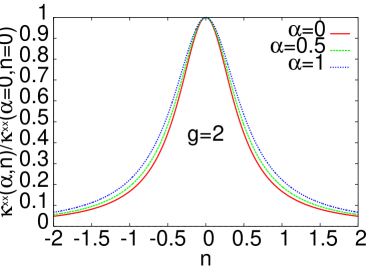
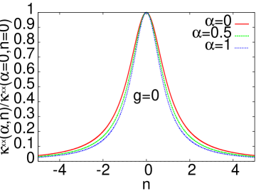
Figure 1: (color online)(left panel) Charge carrier dependence of the thermal conductivity $\kappa^{xx}$, normalized to its $\alpha=0$ value at $n=0$, obtained for the magnetic field $B=0$, mobility $\mu=0.5$, $g=2$ and a few values of $\alpha$. (right panel) The same dependence, except that $g=0$. Note, the $g$ dependent change of the width of curves for various values of $\alpha$ parameters.

As next step of our analysis of the effect of $\alpha$ on transport properties of graphene we show in Fig.2 the dependence of the Wiedemann - Franz ratio (WFR) defined as

$$WFR=W^{xx}=\kappa^{xx}/(\sigma^{xx}T),$$ (72)

where $\sigma^{xx}=\sum_{a,b}^{F,B}\sigma^{xx}_{ab}$. The effect is related to the change of the the width of curves, as well as, their heights. Again the precise analysis of the dependence of $WFR$ on $n$ can be achieved by the appropriate use of both parameters referring to the currents, namely $g$ and $\alpha$. Generally, $WFR$ diminishes with increase of $\alpha$ for all values of the charge density. This change can be attributed to the increase of conductivity or the decrease of resistivity. The latter quantity is shown in the right panel of Fig.2.

In the left panel of Fig.3 we show the dependence of the Seebeck coefficient $S^{xx}$ on the charge concentration $n$ for three systems characterized by different mobilities $\mu=0.5,1$ and $3$. With the increase of mobility $S^{xx}$ gets larger value and its maximum shifts towards smaller carrier concentration. The Seebeck coefficient has been measured in ghahari2016 as a function of gate voltage applied to the graphene sheet. To see the relevance of our calculations it has to be recalled that the charge concentration in graphene can be changed by the external gate voltage. The detailed relation between $n$ and the gate voltage is unknown but is typically of linear character. The dependence of $S$ on the gate voltage measured for different temperatures ghahari2016 and shown in Fig.3 of that paper nicely agrees with our calculations as presented in Fig.3 (left panel). In the figure we plot the Seebeck coefficient for a few values of the mobility parameter $\mu$. The authors of the experiment suggest that the interaction with the optical phonons is responsible for the observed changes of $S$ with temperature. As visible in the discussed figure we observe completely analogous changes with the mobility of the sample in question. This is sensible as in the ultra-pure graphene studied in ghahari2016 the increased interaction with phonons reduces the mobility of the system at higher temperatures. The very good agreement between the experimentally measured data and our calculations can be interpreted in favor of the holographic approach being able to describe real systems studied in the lab.

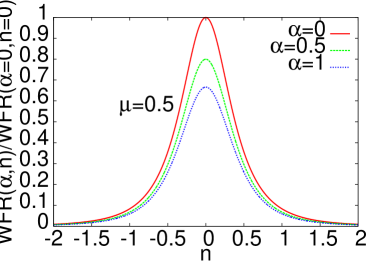
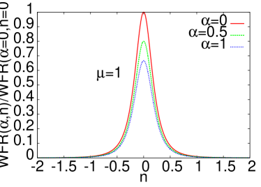
Figure 2: (color online)(left panel) Charge carrier dependence of the Wiedemann-Franz ratio (WFR) normalized to its $\alpha=0$ value at $n=0$ obtained for $B=0$, mobility $\mu=0.5$, $g=2$ and a few values of $\alpha$. (right panel) The same dependence except that $\mu=1$. Note the change of height roughly independent of the mobility and $\mu$ dependent change of width at half maximum.

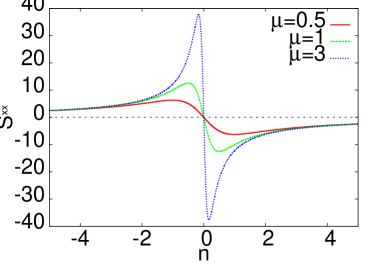
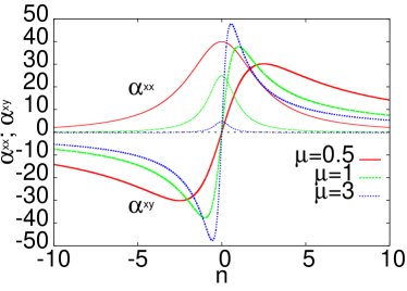
Figure 3: (color online) (left panel) Charge carrier dependence of the Seebeck coefficient $S=S^{xx}$ obtained for $B=0$ and a few values of mobility $\mu$, the parameter which on the gravity side is related to the momentum dissipation $\beta$. (right panel) The kinetic coefficients $\alpha^{xx}$ and $\alpha^{xy}$ $vs.~{}n$ obtained for magnetic field $B=1$ and a few values of $\mu$. The coefficient $\alpha^{xy}$ has been shifted upwards by the constant value 50.

Similarly, very good agreement with the experimentally determined dependence of the coefficients $\alpha^{xx}$ and $\alpha^{xy}$ on the carrier concentration is observed between our data, shown in the right panel of the Fig.3, and the dependence plotted in the Fig.4 of the paper checkelsky2009 . However, to get the agreement with the experimental dependence of $\alpha^{xy}$ we have to shift it vertically by the constant value $50$. This is probably related to the fact that experiment has been performed at high magnetic fields ($B=7T$ and $14T$). At such values of the field the spectrum becomes quantized and the occupied Landau level appears at the Dirac point graph-rev1 ; graph-rev2 . We have not taken into account this effect in our holographic approach davis2008 ; jokela2011 and the above shift corrects for it.

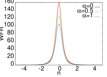
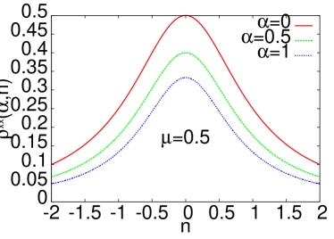
Figure 4: (color online) (left panel) Charge carrier dependence of the Wiedemann-Franz ratio (WFR) obtained for $B=0$, mobility $\mu=0.5$, $g=2$ and a few values of $\alpha$. (right panel) Similar dependence of the diagonal resistivity $\rho^{xx}$ and the same system parameters.

Finally we comment on the $\alpha$ effect on the diagonal resistivity and the Wiedemann-Franz ratio. The charge dependence of these two transport parameters are displayed in Fig.4. Increase of $\alpha$ leads to decrease of both $\rho^{xx}$ and $WFR=W^{xx}$. Again the effect is not very big but well visible and amounts to change of the maximum value of $W^{xx}$ by 20% if the coupling $\alpha$ changes from 0 to 0.5.

It has to be reminded that all transport coefficients of graphene become a two by two matrices if the magnetic field $B$ perpendicular to the layer is applied. The important parameter entering all transport coefficients together with $B$ is the effective mobility $\mu$ related to the holographic parameter $\beta$ responsible for the dissipation of momentum. It is important to notice that the diagonal transport coefficients take on finite values even at zero charge concentration. However, to have non-zero also the off-diagonal elements one has to assume finite values of the charge density. Here we shall assume $n=0.1$. With this value of charge density we are close enough to the particle - hole symmetry point and may analyze the whole matrix of kinetic and transport coefficients. We start with Seebeck $S^{xx}$ and Nernst $S_{xy}$ effects.

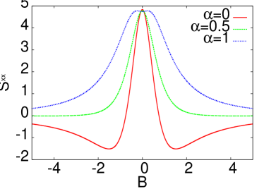
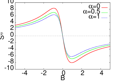
Figure 5: (color online) The Seebeck $S^{xx}$ (left panel) and Nernst $S^{xy}$ (right panel) coefficients calculated for $n=0.1$, $\mu=1$, $g=2$ and a few values of the coupling $\alpha$ as functions of magnetic field $B$.

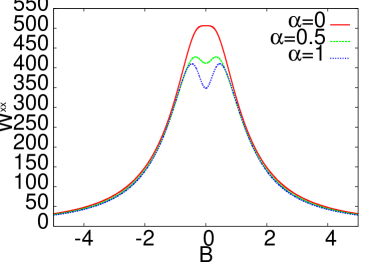
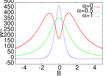
Figure 6: (color online) Magnetic field dependence of the diagonal $WFR$ (left panel) and off-diagonal $WFR^{xy}$ Wiedemann - Franz ratio (right panel) as function of magnetic field $B$ and for a few values of the coupling $\alpha$. Other parameters are set to $\mu=1$ and $g=2$.

Fig.5 illustrates the magnetic field dependence of the Seebeck and Nernst coefficients for moderate value of the mobility $\mu=1$ and for the current mixing parameter $g=2$ (this is close to the value used to describe charge dependence of thermal conductivity in graphene seo17 ). Again we pay special attention to the effect of $\alpha$ on the studied dependencies. It is especially large on the $S^{xx}(B)$ with spectacular change of shape: from the curve with two minima and a maximum for $B=0$ observed for $\alpha=0$ to the curve with a minimum at $B=0$ and two small maxima for larger absolute value of the magnetic field. The Nernst coefficient $S^{xy}$ is an anti-symmetric function of $B$ while $S^{xx}$ is symmetric in $B$.

Typically one measures the Wiedemann-Franz ratio for a system at zero or constant magnetic field varying the charge density. Here we propose the generalization of this parameter in two directions. First, we define both diagonal and off-diagonal parts and second we study it as a function of magnetic field. While $W^{xx}$ is defined in Eq. (72), we define $W^{xy}$ in the simplest possible way as

$$W^{xy}=\frac{\kappa^{xy}}{T\sigma^{xy}}.$$ (73)

We are not aware of any experimental work on graphene studying systematically these parameters as functions of the magnetic field for constant charge density and propose their measurements as a possible check of our theory and holographic analysis of transport in graphene. Such measurements would provide an important hint towards holographic modeling of transport in strongly interacting systems. Our predictions of the magnetic field dependence of $W^{xx}$ and $W^{xy}$ are shown in Fig.6.

VI.1 The Hall angle

In this subsection we shall elaborate the influence of $\alpha$-coupling constant of the two sectors in question on the hall angle. To commence with, let us define the Hall angle, by the ratio of the electric conductivities, in the form provided by

$$\tan\theta=\frac{\sigma^{xx}}{\mid\sigma^{xy}\mid}=\frac{E}{F},$$ (74)

where we have denoted

$$\sigma^{xx} = \sigma_{(FF)}^{xx}+2\sigma_{(FB)}^{xx}+\sigma_{(BB)}^{xx},$$ (75)

$$\sigma^{xy} = \sigma_{(FF)}^{xy}+2\sigma_{(FB)}^{xy}+\sigma_{(BB)}^{xy},$$ (76)

The exact forms of $\sigma_{(ab)}^{ij}$ lead to the following expressions for $E$ and $F$:

$$E = (2+\alpha)[(B^{2}+8\beta^{2}r_{h}^{2})+16B^{2}{\tilde{\mu}}^{2}~{}r_{h}^{6}]+8{\tilde{\mu}}~{}r_{h}^{4}~{}(B^{2}+8\beta^{2}r_{h}^{2})\Big{(}1+\frac{\alpha}{2}\Big{)}^{2}(1+g)^{2}$$

$$+ 32B^{2}{\tilde{\mu}}^{2}~{}r_{h}^{6}~{}\Big{(}1+\frac{\alpha}{2}\Big{)}(1+g)+B^{2}~{}r_{h}^{2}~{}(B^{2}+8\beta^{2}r_{h}^{2}),$$

and

$$F = 32B{\tilde{\mu}}^{3}~{}r_{h}^{7}~{}\Big{(}1+\frac{\alpha}{2}g\Big{)}\Big{(}1+\frac{\alpha}{2}\Big{)}^{2}(1+g)^{2}+8B^{2}{\tilde{\mu}}~{}r_{h}^{5}~{}\Big{(}1+\frac{\alpha}{2}g\Big{)}$$

$$+ 8b{\tilde{\mu}}~{}r_{h}^{3}~{}\Big{(}1+\frac{\alpha}{2}\Big{)}(1+g)(B^{2}+8\beta^{2}r_{h}^{2}).$$

The explicit value of the charge connected with Maxwell field is given by $Q_{(F)}={\tilde{\mu}}~{}r_{h}$. On the other hand, for the radius of black brane one obtains the relation

$$r_{h~{}(1,2)}=\frac{16\pi T\pm\sqrt{(16\pi T)^{2}+48(2\beta^{2}+{\tilde{\mu}}_{all}^{2}+q_{m}^{2})}}{24},$$ (79)

where ${\tilde{\mu}}_{all}={\tilde{\mu}}^{2}+{\tilde{\mu}}_{add}^{2}+\alpha{\tilde{\mu}}{\tilde{\mu}}_{add}$. Thus $r_{h}$ is roughly proportional to the Hawking temperature. From the above expression, it can be seen that in the limit of high temperature, when $\beta$ tends to zero, one gets that $\tan\theta$ increases when $B$ and $\beta$ increase. Moreover for the limit in question we obtain the proportionality of the Hall angle to the inverse of the adequate power of the temperature

$$\tan\theta=c_{0}+\frac{c_{1}}{T}+\frac{c_{2}}{T^{3}}+{\cal O}(1/T^{7}),$$ (80)

where the coefficients are provided by

$$c_{1}=\frac{B~{}(2+\alpha)}{2{\tilde{\mu}}~{}(1+\frac{\alpha}{2}g)(1+\frac{\alpha}{2})^{2}(1+g)^{2}},\qquad c_{2}=\frac{B}{4{\tilde{\mu}}~{}(1+\frac{\alpha}{2}g)}.$$ (81)

The close inspection of the above coefficients reveals, that for a constant value of magnetic and electric field ${\tilde{\mu}}$,  $\alpha>0$ and for $g=0.3$ the dominant role plays the term proportional to $1/T^{3}$. The bigger value of $\alpha$-coupling constant (and/or $g$) one considers, the greater $c_{2}$ is, in comparison to $c_{1}$.

VII Summary and conclusions

We have studied thermoelectric transport properties of graphene assuming that close to the Dirac point the carriers are strongly interacting and thus the gauge-gravity duality is applicable. We consider Hall effect geometry with the magnetic field perpendicular to the graphene plane and with the electric field and temperature gradients in the plane but being perpendicular to each other. The calculation of the DC-transport coefficients is facilitated by the introduction of the axionic field $\beta$ which on the condensed matter side provides momentum relaxation mechanism and, as our calculations show, is related to the mobility of the material. The second sector of $U(1)$-gauge field taken into account in the action affects the kinetic and transport coefficients via the parameters $g$ and $\alpha$.

Having in mind the reference seo17 , our model predicts that the increase of $\alpha$-coupling constant value leads to the increase of the width of normalized thermal conductivity with $g=2$. On the contrary, when $g=0$, the effect is quite opposite, i.e., one obtains the decrease of the width. The dependence of $\alpha$-coupling constant on the Wiedemann-Franz ratio (WFR) is related to the changes of the width of curves and their heights. The general tendency envisaged in the fact that WFR diminishes as $\alpha$-coupling constant increases. The aforementioned dependence is valid for all charge densities.

Based on the model in question we plot the dependence of the Seebeck coefficient on the charge concentration, for the different values of mobilities $\mu$. The mobility increase causes that $S^{xx}$ reaches larger values and its maximum is shifted towards the values of small carrier concentrations. One receives a very good agreement with the experimental data. The same is true for $\alpha^{xx}$ and $\alpha^{xy}$ coefficients.

As far as the charge dependence of the diagonal resistivity and the Wiedemann-Franz ratio on $\alpha$-coupling constant, we reveal that the increase of the coupling constant of two gauge fields causes the decrease of both $\rho^{xx}$ and $W^{xx}$. We also examine the influence of magnetic field on the Seebeck and Nerst coefficients, paying special attention to the $\alpha$-coupling constant effects on the aforementioned phenomena. One finds that the influence is large for $S^{xx}$, changing the shape of the curve, from the curve with two minima and a maximum (for $B=0,~{}\alpha=0$) to the curve with a minimum at $B=0$ and two small maxima for larger absolute values of magnetic field. To our knowledge, this is the new effect, which has not been observed yet. Perhaps future experiments may verify our theoretical predictions.

It also turns out that $\alpha$ influences the Hall angle, causes its increase when magnetic field and $\beta$ increase. In the high temperature regime we observe that $\tan\theta=c_{0}+c_{1}/T+c_{2}/T^{3}+{\cal O}(1/T^{7})$.

However, due to the fact that $\alpha$ modifies the pre-factors only its experimental detection in such measurements will be very hard, if possible at all. The possible exception is provided by the magnetic field dependence of the Seebeck coefficient $S^{xx}$ and the diagonal Wiedemann-Franz ratio $W^{xx}$. The situation might change in the geometry with the in-plane magnetic field. It has to be stressed that our results on the density dependence of the thermoelectric coefficients $\alpha^{xx}$ and $\alpha^{xy}$ and the Seebeck coefficient $S^{xx}$ nicely agree with the experimental data ghahari2016 ; checkelsky2009 .

VII.1 Dark matter interpretation

On the other side, the hope is that experimental studies of various condensed systems allow for checks of the approach and eventually contribute to better understanding of gravity itself. In particular the long standing problem on the gravity side is the direct observation of the dark matter. This elusive component of the Universe is expected to be responsible for more than five times of the mass in the Universe as visible one. The problem is thus serious and worth studying in view of the latest astronomical observations, proposed future investigations and negative or non-conclusive results of the present direct experiments agnes2015 ; til15 ; massey15a ; massey15b ; afa09 ; gni08 ; suz15 ; mir09 ; red13 ; reg15 ; ali15 ; foo15 ; foo15a ; bra14 ; ful15 ; lop14 ; nak12 ; nak15aa ; mun16 aiming at its detection. There has been some efforts to look again into the old astrophysical observations like supernova 1987A data and to try to reinterpret them taking into account the existence of dark radiation (the dark photon) cha17 , as well as, to find the strong constraints on emission of dark photons from stars pos13 and on the coupling of dark matter coming from light particle production in hot star cores and their effects on star cooling har17 . The aforementioned studies are also important in the context of the new rival precession of cosmic microwave background measurements, delivered by Dark Energy Survey (equipped with 570-megapixel camera, able to capture the digital imagines of galaxies at 8 billion light years distances) which supports the view that dark matter and dark energy make up most of our Universe.

One of the directions, we have followed nak14 ; nak15 ; nak15a1 ; rog15 ; rog15a ; rog16a ; rog16b ; rog17 was to analyze the effect of dark matter on the superconducting properties of materials in order to uncover possible effects which could be related to dark sector. The sharpness of the superconducting transition should be helpful to detect even small changes of e.g., transition temperature due to the presence of the dark matter. Generally it is argued that the dark sector affects various properties of the systems pen15 ; pen17 . Studying these changes may contribute to uncover other than gravity effects of dark matter sector.

As noted earlier one can interpret the second field in action (1) as the dark sector coupled to the visible one. Having in mind that the coupling to the dark sector changes only the pre-factors of $Q_{(F)}$ we conclude that in the studied geometry with magnetic field perpendicular to the plane of graphene it will be very difficult, if possible at all, to detect the effect of dark matter experimentally (more details below). The situation might change for the geometry with in-plane magnetic field, as the recent experimental detection of the mixed gauge-gravitational anomaly suggests gooth2017 . This issue is the subject of the on-going studies.

The observed dependence of transport on $g$ and $\alpha$ can be in principle at least utilized in future experiments aiming at the detection of the dark sector. One possible approach could be the long-time observations of the properties of well characterized graphene sample. If the dark matter exists, as required by the astrophysical observations, so it may be spotted during the annual motion of the Earth foo15 -foo15a and freese2013 -kou14 . The possible effect of the dark matter on graphene can in principle be detected by the precise and cleverly designed experiments looking at the annual changes of their transport properties. We rely here on the arguments presented in the aforementioned works, where the authors analyze the annual modulations of the dark matter. Our additional assumption is that dark matter is non-homogeneously distributed in the neighborhood of the Sun frenk2012 ; jungman1996 and these inhomogeneities can be vital for its detection  davoudiasl2012 . The theoretically expected small value of $\alpha$-coupling constant is an important factor making the experiments very difficult, but maybe not impossible.

References

• (1)
• (2)
• (3)
• (4) M.Ammon and J.Erdmenger, Gauge/Gravity Duality. Foundations and Applications, Cambridge University Press (2015).
• (5) J.Zaanen, Y. Sun, Y. Liu, and K.Schalm, Holographic Duality in Condensed Matter Physics, Cambridge University Press (2015).
• (6) J.M.Maldacena, The large-N limit of superconformal field theories and supergravity, Adv. Theor. Math. Phys. 2 (1998) 231.
• (7) E.Witten, Anti-de-Sitter space and holography, Adv. Theor. Math. Phys. 2 (1998) 253.
• (8) S.S.Gubser, I.R.Klebanov and A.M.Polyakov, Gauge theory correlators from noncritical string theory, Phys. Lett. B 428 (1998) 105.
• (9) P. Kovtun, D. Son and A. Starinets, Viscosity in strongly interacting quantum field theories from black hole physics, Phys. Rev. Lett. 94 (2005) 111601.
• (10) P.Romatscke and U.Romatschke, Viscosity information from relativistic nuclear collisions: how perfect is the fluid observed at RHIC, Phys. Rev. Lett. 99 (2007) 172301.
• (11) E. Shuryak, Why does the quark gluon plasma at RHIC behave as a nearly ideal fluid?, Prog. Part. Nucl. Phys. 53, 273 (2004).
• (12) D.Mateos, String theory and quantum chromodynamics, Class. Quant. Grav. 24 (2007) S713.
• (13) S.A.Hartnoll, P.K.Kovtun, M.Mรผller, and S.Sachdev, Theory of the Nerst effect near quantum phase transition in condensed matter and in dyonic black hole, Phys. Rev. B 76 (2007) 144502.
• (14) A.Lucas, J.Crossno, K.C. Fong, P.Kim, and S.Sachdev, Transport in inhomogeneous quantum critical fluids and in the Dirac fluid in graphene, Phys. Rev. B 93 (2016) 075426.
• (15) C.Cao, E.Elliot, J.Joseph, H.Wu, J.Petricka, T.Schรคfer, and J.E.Thomas, Universal Quantum Viscosity in a Unitary Fermi Gas, Science 331, (2011) 58.
• (16) D. A. Bandurin, I. Torre, R. Krishna Kumar, M. Ben Shalom, A. Tomadin, A. Principi, G. H. Auton, E. Khestanova, K. S. Novoselov, I. V. Grigorieva, L. A. Ponomarenko, A. K. Geim, M. Polini, Negative local resistance caused by viscous electron backflow in graphene, Science 351, (2016) 1055.
• (17) J. Crossno, J. K. Shi, K. Wang, X. Liu, A. Harzheim, A. Lucas, S. Sachdev, P. Kim, T. Taniguchi, K. Watanabe, T. A. Ohki, K. C. Fong, Observation of the Dirac fluid and the breakdown of the Wiedemann-Franz law in graphene, Science 351, (2016) 1058.
• (18) P. J. W. Moll, P. Kushwaha, N. Nandi, B. Schmidt, A. P. Mackenzie, Evidence for hydrodynamic electron flow in PdCoO2, Science 351, (2016) 1061.
• (19) J. Zaanen, Electrons go with the flow in exotic material systems, Science 351, (2016) 1026.
• (20) M.Blake and D.Tong, Universal resistivity from holographic massive gravity, Phys. Rev. D 88 (2013) 106004.
• (21) R.A.Davidson, Momentum relaxation in holographic massive gravity, Phys. Rev. D 88 (2013) 086003.
• (22) M.Blake, D.Tong, and D.Vegh, Holographic lattices give the graviton an effective mass, Phys. Rev. Lett. 112 (2014) 071602.
• (23) A.Donos and J.P.Gauntlett, Holographic Q-lattice, JHEP 04 (2014) 040.
• (24) A.Donos and J.P.Gauntlett, Novel metals and insulators from holography, JHEP 06 (2014) 007.
• (25) T.Andrade and B.Withers, A simple holographic model of momentum relaxation, JHEP 05 (2014) 101.
• (26) A.Donos and J.P.Gauntlett, Thermoelectric DC conductivities from black hole horizons, JHEP 11 (2014) 081.
• (27) A.Amoretti, A.Braggio, N.Maggiore, N.Magnoli, and D.Musso, Thermo-electric transport in gauge/gravity models with momentum dissipation, JHEP 09 (2014) 160.
• (28) A.Amoretti, A.Braggio, N.Maggiore, N.Magnoli, and D.Musso, Analytic dc thermoelectric conductivities in holography with massive gravitons, Phys. Rev. D 91 (2015) 025002
• (29) A.Donos and J.P.Gauntlett, Navier-Stokes equations on black hole horizons and DC thermoelectric conductivity, Phys. Rev. D 92 (2015) 121901.
• (30) E.Banks, A.Donos, and J.P.Gauntlett, Thermoelectric DC conductivities and Stokes flows on black hole horizons, JHEP 10 (2015) 103.
• (31) A.Donos, J.P.Gauntlett, T.Griffin, and L.Melgar, DC conductivity of magnetised holographic matter, JHEP 01 (2016) 113.
• (32) A.Donos, J.P.Gauntlett, T.Griffin, and L.Melgar, DC conductivity and higher derivative gravity hep-th 1701.01389 (2017).
• (33) L.Cheng, X.H.Ge, and Z.Y.Sun, Thermoelectric DC conductivities with momentum dissipation from higher derivative gravity, JHEP 04 (2015) 135.
• (34) M.Blake, A.Donos, and N.Lohitsiri, Magnetothermoelectric response from holography, JHEP 08 (2015) 124.
• (35) M.Blake and A.Donos, Quantum critical transport and the Hall angle, Phys. Rev. Lett. 114 (2015) 021601.
• (36) A.Amoretti and D.Musso, Magneto-transport from momentum dissipating holography, JHEP 09 (2015) 094.
• (37) A.Lucas and S.Sachdev, Memory matrix theory of magnetotransport in strange metals, Phys. Rev. B 91 (2015) 195122.
• (38) K.Y.Kim, K.K.Kim, Y.Seo, and S.J.Sin, Thermoelectric conductivities at finite magnetic field and the Nerst effect, JHEP 07 (2015) 027.
• (39) M. S. Foster and I. L. Aleinerm, Slow imbalance relaxation and thermoelectric transport in graphene Phys. Rev. B 79, 085415 (2009).
• (40) Y. Seo, G. Song, P. Kim, S. Sachdev, and S.-J. Sin, Holography of the Dirac Fluid in Graphene with Two Currents, Phys. Rev. Lett. 118 (2017) 036601.
• (41) B.S.Acharya, S.A.R.Ellis, G.L.Kane, B.D.Nelson and M.J.Perry, Lightest Visible-Sector Supersymmetric Particle is Likely Unstable, Phys. Rev. Lett. 117 (2016) 181802.
• (42) B.Holdom, Two U(1)โ€™s and $\epsilon$ charge shifts, Phys. Lett. B 166 (1986) 196.
• (43) D.Lรผst, Intersecting brane worlds: a path to the standard model?, Class. Quant. Grav. 21 (2004) S1399.
• (44) S.Abel and J.Santiago, Constraining the string scale: from Planck to weak and back again, J. Phys. G 30 (2004) R83.
• (45) S.A.Abel, M.D.Goodsell, J.Jaceckel, V.V. Khoze, and A.Ringwald, Kinetic mixing term of photon with hidden U(1)s in string phenomenology, JHEP 07 (2008) 124.
• (46) S.A.Abel and B.W.Schofield, Brane-antibrane kinetic mixing term, millicharged particles and SUSY braeking, Nucl. Phys. B 685 (2004) 150.
• (47) K.R.Dienes, C.F.Kolda, J.March-Russel, Kinetic mixing and the supersymmetric gauge hierarchy, Nucl. Phys. B 492 (1997) 104.
• (48) A.Amoretti, A.Braggio, N.Maggiore, N.Magnoli, and D.Musso, Coexistence of two vector order parameters: a holographic model for ferromagnetic superconductivity, JHEP 01 (2014) 054.
• (49) S. Das Sarma, S. Adam, E. H. Hwang, and E. Rossi, Electronic transport in two - dimensional graphene, Rev. Mod. Phys. 83, (2011) 407.
• (50) D.N. Basov, M.M. Fogler, A. Lanzara, F. Wang, and Y. Zhang, Colloquium: Graphene spectroscopy, Rev. Mod. Phys. 86, (2014) 959.
• (51) F. Ghahari, H.-Y. Xie, T. Taniguchi, K. Watanabe, M. S. Foster, and P. Kim, Enhanced Thermoelectric Power in Graphene: Violation of the Mott Relation by Inelastic Scattering, Phys. Rev. Lett. 116 (2016) 136802.
• (52) J. G. Checkelsky and N. P. Ong, Thermopower and Nernst effect in graphene in a magnetic field, Phys. Rev. B 80 (2009) 081413 R.
• (53) J. L. Davis, P. Kraus, and A. Shah, Gravity dual of a quantum Hall plateau transition, JHEP 11 (2008) 020.
• (54) N. Jokela, M. Jarvinenc, and M. Lippert, A holographic quantum Hall model at integer filling, JHEP 05 (2011) 101.
• (55) J. Gooth, A. C. Niemann, T. Meng, A. G. Grushin, K. Landsteiner, B. Gotsmann, F. Menges, M. Schmidt, C. Shekhar, V. Sรผss, R. Hรผhne, B. Rellinghaus, C. Felser, B. Yan and K. Nielsch, Experimental signatures of the mixed axial - gravitational anomaly in the Weyl semimetal NbP, Nature 547, (2017) 324.
• (56) K. Freese, M. Lisanti, and Ch. Savage, Colloquium: Annual modulation of dark matter, Rev. Mod. Phys. 85, (2013) 1561.
• (57) C.Kouvaris and I.M.Shoemaker, Daily modulation as a smoking gun of dark matter with significant stopping rate, Phys. Rev. D 90 (2014) 095011.
• (58) C. S. Frenk and S. D. M. White, Ann. Phys. (Berlin) 524, 507 (2012), Dark matter and cosmic structure.
• (59) G. Jungman, M. Kamionkowski, and K. Griest, Supersymmetric Dark Matter, Phys. Reports 267 (1996) 195.
• (60) H. Davoudiasl, H.-S. Lee, and W. J. Marciano, โ€œDarkโ€ Z implications for parity violation, rare meson decays, and Higgs physics, Phys. Rev. D 85 (2012) 115019.
• (61) P.Agnes, T. Alexander, A.Alton et al., First results from the DarkSide-50 dark matter experiment at Laboratori Nazionali del Gran Sasso, Phys. Lett. B 743 (2015) 456.
• (62) K.Van Tilburg, N.Leefer, L.Bougas, and D.Budker, Search for Ultralight Scalar Dark Matter with Atomic Spectroscopy, Phys. Rev. Lett. 115 (2015) 011802.
• (63) D.Harvey, R.Massey, T.Kitching, A.Taylor and E.Tittley, The nongravitational interactions of dark matter in colliding galaxy clusters, Science 347, (2015) 1462.
• (64) R.Massey et al., The behaviour of dark matter associated with four bright cluster galaxies in the 10 kpc core of Abell 3827, Mon. Not. R. Astr. Soc. 449 (2015) 3393.
• (65) A.Afanasev, O.K. Baker, K.B.Beard, G.Biallas, J.Boyce, M.Minarni, R.Ramdon, M.Shinn, and P.Slocum, New experimental limit on photon hidden-sector paraphoton mixing, Phys. Lett. B 679 (2009) 317.
• (66) S. N. Gninenko and J.Redondo, On search for EV hidden-sector in Supper-Kanionkande and CAST experiments, Phys. Lett. B 664 (2008) 180.
• (67) J.Suzuki, T.Horie, Y.Inoue, and M.Minowa, Experimental search for hidden photon CDM in the eV mass range with a dish antenna, JCAP 09, (2015) 042.
• (68) A.Mirizzi, J.Redondo, and G.Sigl, Microwave background constraints on mixing of photons with hidden photons, JCAP 03, (2009) 026.
• (69) J.Redondo and G.Raffelt, Solar constraints on hidden photons re-visited, JCAP 08, (2013) 034.
• (70) M.Regis, J.Q.Xia, A.Cuoso, E.Branchini, N.Fornengo, and M.Viel, Particle Dark Matter Searches Outside the Local Group, Phys. Rev. Lett. 114 (2015) 241301.
• (71) Y.Ali-Haimoud, J.Chluba, and M.Kamionkowski, Constraints on Dark Matter Interactions with Standard Model Particles from Cosmic Microwave Background Spectral Distortions, Phys. Rev. Lett. 115 (2015) 071304.
• (72) R.Foot and S.Vagnozzi, Dissipative hidden sector dark matter, Phys. Rev. D 91 (2015) 023512.
• (73) R.Foot and S.Vagnozzi, Diurnal modulation signal from dissipative hidden sector dark matter, Phys. Lett. B 748 (2015) 61.
• (74) J.Bramante and T.Linden, Detecting dark matter with imploding pulsars in the galactic center, Phys. Rev. Lett. 113 (2014) 191301.
• (75) J.Fuller and C.D.Ott, Dark-matter-induced collapse of neutron stars: a possible link between fast radio bursts and missing pulsar problem, Mon. Not. R. Astr. Soc. 450 (2015) L71.
• (76) I.Lopes and J.Silk, A particle dark matter footprint on the first generation of stars, Astrophys. J. 786 (2014) 25.
• (77) A.Nakonieczna, M.Rogatko, and R.Moderski, Dynamical collapse of charged scalar field in phantom gravity, Phys. Rev. D 86 (2012) 044043.
• (78) A.Nakonieczna, M.Rogatko, and L.Nakonieczny, Dark matter impact on gravitational collapse of an electrically charged scalar field, JHEP 11 (2015) 016.
• (79) J.B. Munoz, E.D. Kovetz, L. Dai, and M. Kamionkowski, Lensing of Fast Radio Bursts as a Probe of Compact Dark Matter, Phys. Rev. Lett. 117 (2016) 091301.
• (80) J.ย H. Chang, R.ย Essig, and S.ย D. McDermott, Revisiting supernova 1987a constraints on dark photons, JHEP 1 (2017) 107.
• (81) H.An, M.Pospelov, and J.Pradler, New stellar constraints on dark photons, Phys. Lett. B 725 (2013) 190.
• (82) E.Hardy and R.Lasenby, Stellar cooling bounds on new light particles: plasma mixing effects, JHEP 02 (2017) 033.
• (83) ล.Nakonieczny and M.Rogatko, Analytic study on backreacting holographic superconductors with dark matter sector, Phys. Rev. D 90 (2014) 106004.
• (84) ล.Nakonieczny, M.Rogatko and K.I. Wysokiล„ski, Magnetic field in holographic superconductors with dark matter sector, Phys. Rev. D 91 (2015) 046007.
• (85) ล. Nakonieczny, M. Rogatko and K.I. Wysokiล„ski, Analytic investigation of holographic phase transitions influenced by dark matter sector, Phys. Rev. D 92 (2015) 066008.
• (86) M. Rogatko, K.I. Wysokiล„ski, P-wave holographic superconductor/insulator phase transitions affected by dark matter sector, JHEP 03 (2016) 215.
• (87) M. Rogatko, K.I. Wysokiล„ski, Holographic vortices in the presence of dark matter sector, JHEP 12 (2015) 041.
• (88) M. Rogatko, K.I. Wysokiล„ski, Viscosity of holographic fluid in the presence of dark matter sector, JHEP 08 (2016) 124.
• (89) M. Rogatko, K.I. Wysokiล„ski, Condensate flow in holographic models in the presence of dark matter, JHEP 10 (2016) 152.
• (90) M. Rogatko, K.I. Wysokiล„ski, Viscosity bound for anisotropic superfluids with dark matter sector, Phys. Rev. D 96 (2017) 026015.
• (91) Y.Peng, Holographic entanglement entropy in superconductor phase transition with dark matter sector, Phys. Lett. B 750 (2015) 420.
• (92) Y.Peng, Q.Pan and Y.Liu, A general holographic insulator/superconductor model with dark matter sector away from the probe limit, Nucl. Phys. B 915 (2017) 69.