A Semi-smooth Newton Method For Solving semidefinite programs in electronic structure calculations

Abstract

The ground state energy of a many-electron system can be approximated by an variational approach in which the total energy of the system is minimized with respect to one and two-body reduced density matrices (RDM) instead of many-electron wavefunctions. This problem can be formulated as a semidefinite programming problem. Due the large size of the problem, the well-known interior point method can only be used to tackle problems with a few atoms. First-order methods such as the the alternating direction method of multipliers (ADMM) have much lower computational cost per iteration. However, their convergence can be slow, especially for obtaining highly accurate approximations. In this paper, we present a practical and efficient second-order semi-smooth Newton type method for solving the SDP formulation of the energy minimization problem. We discuss a number of techniques that can be used to improve the computational efficiency of the method and achieve global convergence. Extensive numerical experiments show that our approach is competitive to the state-of-the-art methods in terms of both accuracy and speed.

1 Introduction

The molecular Schrödinger’s equation, which is a many-body eigenvalue problem, is a fundamental problem to solve in quantum chemistry. Because the eigenfunction to be determined is a function of $3N$ spatial variables, where $N$ is the number of electrons in a molecule, a brute force approach to solving this equation is prohibitively costly. The most commonly used approaches to obtaining an approximate solution, such as the configuration interaction [27] and coupled cluster methods [32], express the approximate eigenfunction as a linear or nonlinear combination of a set of many-body basis functions (i.e. Slater determinants), and determine the expansion coefficients by solving a projected eigenvalue problem or a set of nonlinear equations. One has to choose the set of many-body basis functions judiciously to balance the computational cost and the accuracy of the approximation. To reach chemical accuracy, the number of basis functions can still grow rapidly with respect to $N$.

An alternative way to approximate the ground state energy (i.e., the smallest eigenvalue), which does not involve approximating the many-body eigenfunction directly, is to reformulate the problem as a convex optimization problem and express the ground state energy in terms of the so called one-body reduced density matrix (1-RDM) and two-body reduced density matrix (2-RDM) that satisfy a number of linear constraints. This convex optimization problem is a semidefinite program (SDP) that can be solved by a number of numerical algorithms to be presented below. This approach is often referred to as the variational 2-RDM (v2-RDM) or 2-RDM method in short.

The development of the 2-RDM method dates back to 1950s. Mayer [17] showed how the energy of a many-body problem can be represented in terms of 1-RDM and 2-RDM, which can be write as a matrix and a 4-order tensor. However, since not all matrices or tensors are RDMs associated with an $N$-electron wavefunction, one must add some constraints to guarantee that the matrices and tensors satisfy the so called N-representability condition, which was first proposed by Coleman [6] in 1963 and has been investigated for nearly 50 years. The N-representability condition for the 1-RDM in the variational problem has been solved in [6]. In 1964, Garrod and Percus [13] showed a sufficient and necessary condition for the 2-RDM N-representability problem. It is theoretically meaningful but computationally intractable. In 2007, Liu et al. showed that the N-representability problem of 2-RDM is QMA-complete [16]. Since then a number of approximation conditions, including the P, Q, R, T1, T2, T2’ conditions, have been proposed in [6, 13, 11, 37, 18, 3]. All these conditions are formulated by keeping matrices whose elements are linear combinations of the components of the 1-RDM and 2-RDM matrices positive semidefinite. As a result, the constrained minimization of the total energy with respect to 1-RDM and 2-RDM becomes a SDP.

The practical use of the v2-RDM approach to solving the ground state electronic structure is enabled, to some extent, by the recent advances in numerical methods for solving large-scale SDPs. In [22], Nakata et al. solved the v2-RDM problem by an interior point method. Zhao et al. reformulated the 2-RDM using the dual SDP formalism and also applied the interior point method in [37]. The problem size of the SDP formulation in [37] is usually smaller than the ones given in [22]. Rigorous error bounds for approximate solutions obtained from the v2-RDM approach are discussed in [4]. Since the computational cost of the interior point method is typically high, this approach has only been successfully used for a handful of small molecules with a few atoms. First order methods, which have much lower complexity per iteration, have gained wide acceptance in recent years. The well-known alternating direction multiplier method (ADMM) has been used to solve general SDPs in [33]. It is the basis of the boundary point method developed by Mazziotti to solve the v2-RDM in [19]. Although ADMM has relatively low complexity per iteration, it may converge slowly and take thousands or tens of thousands iterations to reach high accuracy. Recently, some new methods have been developed to speed up the solution of general SDPs. An example is the Newton-CG Augmented Lagrangian Method for SDP (SDPNAL) proposed in [36]. An enhanced version of SDPNAL called SDPNAL+ is developed in [35], which can efficiently treat nonnegative SDP matrices. However, these methods have not been applied to the v2-RDM approach for electronic structure calculation.

In this paper, we first review how the ADMM method is used to solve the SDP formulation of the v2-RDM given in [37] since it serves as the foundation of the second-order method to be introduced below. We point out a key observation that applying the ADMM to the dual SDP formulation is equivalent to applying the Douglas Rachford splitting (DRS) [8, 15, 10] method to the primal SDP formulation of the problem. The DRS method can be viewed as a fixed point iteration that yields a solution of a system of semi-smooth and monotone nonlinear equations that coincides with the solution of the corresponding SDP. The generalized Jacobian of this system of nonlinear equations is positive semidefinite and bounded. It has a special structure that allows us to compute the Newton step in our semi-smooth Newton method for solving SDPs efficiently. We apply the semi-smooth Newton method to the v2-RDM formulation of the ground state energy minimization problem, and use a hyperplane projection technique [28] to guarantee the global convergence of the method due to the monotonicity of the system of nonlinear equations. Our method is different from SDPNAL [36] and SDPNAL+ [35] which minimizes a sequence of augmented Lagrangian functions for the dual SDP by a semi-smooth Newton-CG method. To improve the computational efficiency for solving v2-RDM problem, we exploit the special structures of matrices resulting from the 1-RDM and 2-RDM constraints. The block diagonal and low rank structures of these matrices are related to spin and spatial symmetry of the molecular orbitals [14, 22, 37]. We show how they can be used to significantly reduce the computational costs in the semi-smooth Newton method. Finally, we implement our codes based on the key implementation details and subroutines of SDPNAL [36], SDPNAL+ [4] and ADMM+ [30]. Extensive numerical experiments on examples taken from [21] to demonstrate that our semi-smooth algorithm can indeed achieve higher accuracy than the ADMM method. We also show that it is competitive with SDPNAL and SDPNAL+ in terms of both computational time and accuracy.

The rest of this paper is organized as follows. In section 2, we provide some background on electronic structure calculation, establish the notation and introduce the v2-RDM formulation. In section 3, we review first order methods suitable for solving the SDP problem arising in the v2-RDM formulation. In particular, we examine the relationship between the ADMM and the DRS. We present a semi-smooth Newton method for solving the v2-RDM in section 4. Numerical results are reported in section 5. Finally, we conclude the paper in section 6.

2 Background

2.1 The variational 2-RDM formulation of the electronic structure problem

The electronic structure of a molecule can be determined by the solution to an $N$-electron Schrödinger equation

(1) $$H\Psi=E\Psi,$$

where $\Psi:\mathbb{R}^{3N}\otimes\{\pm\frac{1}{2}\}^{3N}\rightarrow\mathbb{C}$ is a N-electron antisymmetric wave function that obeys the Pauli exclusion principle, $E$ represent the total energy of the $N$-electron system, and $H$ is the molecular Hamiltonian operator defined by

(2) $$H=\underbrace{\sum_{i=1}^{N}-\frac{1}{2}\triangle_{i}-\sum_{i=1}^{N}\sum_{k=1}^{K}\frac{Z_{k}}{|R_{k}-r_{i}|}}_{\text{one-body term}}+\underbrace{\frac{1}{2}\sum_{i,j=1,\\ i\neq j}^{N}\frac{1}{|r_{i}-r_{j}|}}_{\text{two-body term}}.$$

Here $\triangle_{i}$ denotes a Laplace operator with respect to the spatial coordinate of the $i$-th electrons, $R_{k},k=1,\cdots,K$, gives the coordinates of the $k$-th nuclei with charge $Z_{k}$, and $r_{i},i=1,\cdots,N$, gives the coordinates of the $i$-th electron.

To simplify notation, let us ignore the spin degree of freedom. In this case, the wave function $\Psi$ belongs to the the Hilbert space $L_{2}((\mathbb{R}^{3})^{N})$ endowed with the inner product

$$\left\langle{\Psi_{1}},{\Psi_{2}}\right\rangle=\sum_{s=\pm\frac{1}{2}}\int_{\mathbb{R}^{3N}}\overline{\Psi_{1}(r_{1},\cdots,r_{N})}\Psi_{2}(r_{1},\cdots,r_{N})dr_{1}\cdots dr_{N}.$$

The smallest eigenvalue of $H$, often denoted by $E_{0}$, is called the ground state energy (1).

Solving (1) directly is not computationally feasible except for $N=1$ or $N=2$. A commonly used approach in quantum chemistry is to approximate $\Psi$ from a configuration interaction subspace spanned by a set of many-body basis function $\Phi_{i}$, often chosen to be Slater determinants of the form

(3) $$\Phi_{i}(r_{1},r_{2},\ldots,r_{N})=\frac{1}{\sqrt{N!}}\begin{vmatrix}\phi_{i_{1}}(r_{1})&\phi_{i_{2}}(r_{1})&\ldots&\phi_{i_{N}}(r_{1})\\ \phi_{i_{1}}(r_{2})&\phi_{i_{2}}(r_{2})&\ldots&\phi_{i_{N}}(r_{2})\\ \vdots&\vdots&&\vdots\\ \phi_{i_{1}}(r_{N})&\phi_{i_{2}}(r_{N})&\ldots&\phi_{i_{N}}(r_{N})\end{vmatrix},$$

where $\{\phi_{i}(r\}$ is a set of orthonormal basis functions known as molecular orbitals [26]. These orbitals can be obtained by substituting (3) into (1) and solving a nonlinear eigenvalue problem known as the Hartree-Fock (HF) equation. The $N$ eigenfunctions associated with the smallest $N$ eigenvalues are known as the occupied HF orbitals. All other eigenfunctions are called unoccupied or virtual orbitals. The Slater determinant that consists of the $N$ occupied HF orbitals is called the HF Slater determinant, and denoted by $\Phi_{0}$.

A new Slater determinant can be generated from an existing Slater determinant by replacing one or more orbitals with others. This process is often conveniently expressed through the use of creation and annihilation operators denoted by $\mathbf{a}_{i}^{+}$ and $\mathbf{a}_{i}$ respectively [31]. The successive applications of different combinations of creation and annihilation operators to the HF Slater determinant that replace occupied orbitals with unoccupied orbitals allow us to generate a set of Slater determinants that can be used to expand an approximate solution to (1). The entire set of such Slater determinants defines the so called full configuration interaction (FCI) space. The FCI approximation to the solution of (1) is often used as the baseline for assessing the accuracy of approximate solutions to (1). The size of the FCI space depends on the number of electrons $N$ and the number of degrees of freedom ($d$) used to discretize each orbital $\phi_{i}$ (i.e., the basis set size in the quantum chemistry language). When $N$ is large and an accurate basis set is used to discretize $\phi_{i}$, the FCI space can be extremely large. Hence, FCI calculation can only be performed for small molecules in a small basis set.

The matrix representation of the many-body Hamiltonian (2) in the space of Slater determinants is determined by one electron integrals

$$T_{i,j}=\int_{\mathbb{R}^{3}}\overline{\phi_{i}(r)}(-\frac{1}{2}\triangle-\sum_{c=1}^{K}\frac{Z_{c}}{|r-R_{c}|})\phi_{j}(r)dr,$$

and two electron integrals

$$V_{ij,kl}=\frac{1}{2}\int_{\mathbb{R}^{3}}\int_{\mathbb{R}^{3}}\overline{\phi_{i}(r)\phi_{j}(r^{\prime})}\frac{1}{|r^{\prime}-r|}\phi_{k}(r)\phi_{l}(r^{\prime})drdr^{\prime}.$$

These integrals can be used to express the many-body Hamiltonian (2) using the so called second quantization notation:

(4) $$\mathbf{H}=\sum_{i,j}^{d}T_{i,j}\mathbf{a}_{i}^{+}\mathbf{a}_{j}+\sum_{i,j,k,l=1}^{d}V_{ij,kl}\mathbf{a}_{i}^{+}\mathbf{a}_{j}^{+}\mathbf{a}_{l}\mathbf{a}_{k}.$$

It is well known that the smallest eigenvalue of $\mathbf{H}$ can be obtained from the Rayleigh-Ritz variational principle via the solution of the following constrained minimization problem:

(5) $$E_{0}=\min\left\langle{\Psi},{\mathbf{H}\Psi}\right\rangle\,\textrm{s.t.}\,\left\langle{\Psi},{\Psi}\right\rangle=1.$$

When $\Psi$ is expanded in terms of Slater determinants, substituting (4) into (5) yields

(6) $$E = \left\langle{\Psi},{\mathbf{H}\Psi}\right\rangle=\sum_{i,j}^{d}T_{i,j}\gamma_{i,j}+\sum_{i,j,k,l=1}^{d}V_{ij,kl}\Gamma_{ij,kl},$$

where

(7) $$\gamma_{i,j}=\left\langle{\Psi},{\mathbf{a}_{i}^{+}\mathbf{a}_{j}\Psi}\right\rangle\ \ \mbox{and}\ \ \Gamma_{ij,kl}=\left\langle{\Psi},{\mathbf{a}_{i}^{+}\mathbf{a}_{j}^{+}\mathbf{a}_{l}\mathbf{a}_{k}\Psi}\right\rangle$$

are elements of the so-called one-body reduced density matrix (1-RDM) $\gamma$ and two-body reduced density matrix (2-RDM) $\Gamma$, respectively.

Note that the dimensions of $\gamma$ and $\Gamma$ are $d\times d$ and $d^{2}\times d^{2}$ respectively, where $d$ is proportional to the number of electrons $N$. By treating the total energy $E$ as a function of $\gamma$ and $\Gamma$, we can obtain an approximation to the ground state energy by solving an optimization problem with $O(N^{4})$ variables instead of an eigenvalue problem of a dimension that grows exponentially with respect to $N$.

However, $\gamma$ and $\Gamma$ are not arbitrary matrices. They are said to be $N$-representible if they can be written as (7) for some many-body wavefunction $\Psi$. $N$-representible matrices are known to have a number of properties [18, 37] that can be used to constrain the set of matrices over which the objective function (6) is minimized. These properties include

(8) $$\gamma_{i,j}=\gamma_{j,i},\Gamma_{ij,kl} = \Gamma_{kl,ij};\quad\quad\quad\quad\mbox{Hermitian}$$

(9) $$\Gamma_{ij,kl}=-\Gamma_{ji,kl} = -\Gamma_{ij,lk};\quad\quad\quad\;\mbox{anti-symmetric }$$

(10) $$\mathrm{tr}(\gamma)=N\ \ \mbox{and}\ \ \mathrm{tr}(\Gamma) = \frac{N(N-1)}{2};\quad\;\;\mbox{trace }$$

(11) $$\sum_{k}\Gamma_{ik,jk} = \frac{N-1}{2}\gamma_{ij}.\quad\quad\mbox{ partial trace}$$

However, the above conditions are not sufficient to guarantee $\gamma$ and $\Gamma$ to be $N$-representible. A significant amount of effort has been devoted in the last few decades to develop additional conditions that further constrain $\gamma$ and $\Gamma$ to be $N$-representible [18, 37] without making use of $\Psi$ explicitly. These conditions are collectively called the N-representability conditions.

2.2 N-representability conditions

The N-representability conditions were first introduced in [6]. It has been shown in [6] that $\gamma$ is N-representable if and only if $0\preceq\gamma\preceq I$. For 2-RDM, it is more difficult to write down a complete set of the conditions under which $\Gamma$ is $N$-representable. Liu et al. showed that the N-representability problem is QMA-complete in [16]. There has been efforts to derive approximation conditions that are useful in practice. The well known approximation conditions in [6, 13, 11, 37, 18, 3] define the so-called $P,Q,R,T1,T2$ variables whose elements can be expressed as a linear function with respect to the elements of $\gamma$ and $\Gamma$ as follows:

(12) $$P_{ij,i^{\prime}j^{\prime}} = \left\langle{\Psi},{\mathbf{a}_{i}^{+}\mathbf{a}_{j}^{+}\mathbf{a}_{j}^{\prime}\mathbf{a}_{i}^{\prime}\Psi}\right\rangle=\Gamma_{ij,i^{\prime}j^{\prime}},$$

$$Q_{ij,i^{\prime}j^{\prime}} = \left\langle{\Psi},{\mathbf{a}_{i}\mathbf{a}_{j}\mathbf{a}_{j^{\prime}}^{+}\mathbf{a}_{i^{\prime}}^{+}\Psi}\right\rangle=(\delta_{ii^{\prime}}\delta_{jj^{\prime}}-\delta_{ij^{\prime}}\delta_{ji^{\prime}})-(\delta_{ii^{\prime}}\gamma_{jj^{\prime}}+\delta_{jj^{\prime}}\gamma_{ii^{\prime}})$$

$$+ (\delta_{ij^{\prime}}\gamma_{ji^{\prime}}+\delta_{ji^{\prime}}\gamma_{ij^{\prime}})+\Gamma_{ij,i^{\prime}j^{\prime}},$$

(14) $$G_{ij,i^{\prime}j^{\prime}} = \left\langle{\Psi},{\mathbf{a}_{i}^{+}\mathbf{a}_{j}\mathbf{a}_{j^{\prime}}^{+}\mathbf{a}_{i^{\prime}}\Psi}\right\rangle=\delta_{jj^{\prime}}\gamma_{ii^{\prime}}-\Gamma_{ij^{\prime},i^{\prime}j}$$

(15) $${T1}_{ijk,i^{\prime}j^{\prime}k^{\prime}} = \left\langle{\Psi},{(\mathbf{a}_{i}^{+}\mathbf{a}_{j}^{+}\mathbf{a}_{k}^{+}\mathbf{a}_{k^{\prime}}\mathbf{a}_{j^{\prime}}\mathbf{a}_{i^{\prime}}+\mathbf{a}_{i}\mathbf{a}_{j}\mathbf{a}_{k}\mathbf{a}_{k^{\prime}}^{+}\mathbf{a}_{j^{\prime}}^{+}\mathbf{a}_{i^{\prime}}^{+})\Psi}\right\rangle,$$

$$= \mathcal{A}[ijk]\mathcal{A}[i^{\prime}j^{\prime}k^{\prime}](\frac{1}{6}\delta_{ii^{\prime}}\delta_{jj^{\prime}}\delta_{kk^{\prime}}-\frac{1}{2}\delta_{ii^{\prime}}\delta_{jj^{\prime}}\gamma_{k,k^{\prime}}+\frac{1}{4}\delta_{ii^{\prime}}\Gamma_{jk,j^{\prime}k^{\prime}}),$$

(16) $${T2}_{ijk,i^{\prime}j^{\prime}k^{\prime}} = \left\langle{\Psi},{(\mathbf{a}_{i}^{+}\mathbf{a}_{j}^{+}\mathbf{a}_{k}\mathbf{a}_{k^{\prime}}^{+}\mathbf{a}_{j^{\prime}}\mathbf{a}_{i^{\prime}}+\mathbf{a}_{i}^{+}\mathbf{a}_{j}\mathbf{a}_{k}\mathbf{a}_{k^{\prime}}^{+}\mathbf{a}_{j^{\prime}}^{+}\mathbf{a}_{i^{\prime}})\Psi}\right\rangle$$

$$= \mathcal{A}[jk]\mathcal{A}[j^{\prime}k^{\prime}](\frac{1}{2}\delta_{jj^{\prime}}\delta_{k,k^{\prime}}\gamma_{ii^{\prime}}+\frac{1}{4}\delta_{ii^{\prime}}\Gamma_{j^{\prime}k^{\prime},jk}-\delta_{jj^{\prime}}\Gamma_{ik^{\prime},i^{\prime}k}),$$

where $\delta$ is the Kronecker delta symbol and $\mathcal{A}[ijk]f(i,j,k)=f(i,j,k)+f(j,k,i)+f(k,i,j)-f(i,k,j)-f(j,i,k)-f(k,j,i)$. The $T2$ variable can be strengthened to yield the $T2^{\prime}$ variable described in [3, 18]. We should point out that each of (12)-(16) is in fact a set of equations enumerating all possible indices $i,j,k,i^{\prime},j^{\prime}$ and $k^{\prime}$. Since $\Gamma$ is a $4$-dimensional tensor satisfying (8) and (9), one can convert it to a two-dimensional matrix $\tilde{\Gamma}$, i.e.,

$$\Gamma_{ij,i^{\prime}j^{\prime}}=\tilde{\Gamma}_{j-i+(2d-i)(i-1)/2,j^{\prime}-i^{\prime}+(2d-i^{\prime})(i^{\prime}-1)/2}.$$

Similar properties hold for $Q$. Hence, $\Gamma$ and $Q$ can be transformed into $\frac{d(d-1)}{2}\times\frac{d(d-1)}{2}$ matrices. Because (9) is not satisfied on the $4$-dimensional tensor $G$, it can only be transformed into a $d^{2}\times d^{2}$ matrix. By the anti-symmetric properties of the $6$-dimensional tensors $T1$, $T2$ and $T2^{\prime}$ [37, 3, 18], they can be transformed into $\frac{d(d-1)(d-2)}{6}\times\frac{d(d-1)(d-2)}{6}$, $\frac{d^{2}(d-1)}{2}\times\frac{d^{2}(d-1)}{2}$ and $\frac{d^{2}(d-1)+2d}{2}\times\frac{d^{2}(d-1)+2d}{2}$ matrices, respectively. For simplicity, we still use the notations $\Gamma,P,Q,G,T1,T2$ and $T2^{\prime}$ to represent the matrices translated from these tensors. Finally, the corresponding N-representability condition of (12)-(16) is to require each matrix to be positive semidefinite.

2.3 The SDP formulations

Let $b=(\mathrm{svec}(T),\mathrm{svec}(V))^{T}\in\mathbb{R}^{m}$ and
$y=(\mathrm{svec}(\gamma),\mathrm{svec}(\Gamma))^{T}\in\mathbb{R}^{m}$ be vectorized integral and reduced density matrices that appear in (6) respectively, where $\mathrm{svec}$ is used to turn a symmetric matrix $U$ into a vector according to

$$\mathrm{svec}(U)=(U_{11},\sqrt{2}U_{12},U_{22},\sqrt{2}U_{13},\sqrt{2}U_{23},U_{33},\cdots,U_{nn}).$$

To simplify notations later, we rename matrices as $S_{1}=\gamma$, $S_{2}=P$, $S_{3}=Q$, $S_{4}=G$, $S_{5}=T1$ and $S_{6}=T2$, and treat both $y$ and $\{S_{j}\}$ as variables in the SDP formulation. Using the definition of $y$, we can rewrite the equation $S_{1}=\gamma$ as a system of linear equations

(17) $$S_{1}=\mathcal{A}_{1}^{*}y+C_{1},$$

where $\mathcal{A}_{1}^{*}y=\sum_{p=1}^{m}A_{1p}y_{p}\in\mathbb{R}^{s_{1}\times s_{1}}$ with $A_{1p}\in\mathbb{R}^{s_{1}\times s_{1}}$ and $C_{1}\in\mathbb{R}^{s_{1}\times s_{1}}$. Obviously, $s_{1}=d$ and $C_{1}$ is a zero matrix. Similarly, each of (12)-(16) can be written succinctly as

(18) $$S_{j}=\mathcal{A}_{j}^{*}y-C_{j},\;j=2,\ldots,l=6,$$

where $\mathcal{A}_{j}^{*}y=\sum_{p=1}^{m}A_{jp}y_{p}$ with $A_{jp}\in\mathbb{R}^{s_{j}\times s_{j}}$ and $C_{j}\in\mathbb{R}^{s_{j}\times s_{j}}$. The integer $s_{j}$ is equal to the matrix size of $S_{j}$. The matrices $A_{jp}$ are coefficients matrices of $y_{p}$ and $C_{j}$ are constant matrices in the corresponding equation of (12)-(16).

Using these notations, we can formulate the constrained minimization of (6) subject to $N$-representability conditions as a SDP:

(19) $$\begin{split}\min_{y,S_{j}}\ &b^{T}y\\ \,\textrm{s.t.}\,\ &S_{j}=\mathcal{A}_{j}^{*}y-C_{j},j=1,\cdots,l,\\ &B^{T}y=c,\\ &0\preceq S_{1}\preceq I,\\ &S_{j}\succeq 0,j=2,\cdots,l,\\ \end{split}$$

where the linear constraints $B^{T}y=c$ follows from the conditions (10)-(11) and other equality conditions introduced in [37]. If some of conditions in (12)-(16) are not considered, then (19) can be adjusted accordingly. If the condition on $T2$ is replaced by that of $T2^{\prime}$, then we set $S_{6}=T2^{\prime}$.

The SDP problem given in (19) is often known as the dual formulation. The corresponding primal SDP of (19) is

(20) $$\begin{split}\max_{X_{j},U}\ &\sum_{j=1}^{l}\left\langle{C_{j}},{X_{j}}\right\rangle+\left\langle{c},{x}\right\rangle-\left\langle{C_{1}+I},{U}\right\rangle\\ \,\textrm{s.t.}\,\ &\sum_{j=1}^{l}\mathcal{A}_{j}(X_{j})+Bx-\mathcal{A}_{1}(U)=b,\\ &X_{j}\succeq 0,j=1,\cdots,l,\\ &U\succeq 0,\end{split}$$

where $X_{j}\in\mathbb{R}^{s_{j}\times s_{j}}$, $U\in\mathbb{R}^{s_{1}\times s_{1}}$, $\mathcal{A}_{j}$ is the conjugated operator of $\mathcal{A}_{j}^{*}$ and $\mathcal{A}_{j}(X)=(\left\langle{A_{j1}},{X}\right\rangle,\cdots,\left\langle{A_{jm}},{X}\right\rangle)^{T}$ for any matrix $X\in\mathbb{R}^{s_{j}\times s_{j}}$.

Since the largest matrix dimension of $X_{j}$ and $S_{j}$ is of order $O(d^{3})$ and $m=O(d^{4})$, problems (19) and (20) are large scale SDPs even for a moderate value $d$. However, the $S_{j}$ in (19) are block diagonal matrices due to the spatial and spin symmetries of molecules. Hence, the computational cost for solving (19) can be reduced by exploiting such block diagonal structures. In Table 1, we list the number of diagonal blocks and their dimensions resulting from spin symmetries in each of $\gamma$, $\Gamma,Q,G,T1,T2,T2^{\prime}$ matrices.

Table 1: the matrix dimensions of the block diagonal structures

$S_{j}$ matrix	block dimension
$\gamma$	$\frac{d}{2}$, 2 blocks;
$P$, $Q$, $\Gamma$	$\frac{d^{2}}{4}$, 1 blocks; $\frac{d}{4}(\frac{d}{2}-1)$, 2 blocks;
$G$	$\frac{d^{2}}{2}$, 1 blocks; $\frac{d^{2}}{4}$, 2 blocks;
$T1$	$\frac{d^{2}}{8}(\frac{d}{2}-1)$, 2 blocks; $\frac{d^{2}}{12}(\frac{d}{2}-1)(\frac{d}{2}-2)$, 2 blocks;
$T2$	$\frac{d^{2}}{8}(\frac{3d}{2}-1)$, 2 blocks; $\frac{d^{2}}{8}(\frac{d}{2}-1)$, 2 blocks;
$T2^{\prime}$	$\frac{d}{2}+\frac{d^{2}}{8}(\frac{3d}{2}-1)$, 2 blocks; $\frac{d^{2}}{8}(\frac{d}{2}-1)$, 2 blocks;

Spatial symmetry may lead to additional block diagonal structures within each spin diagonal block listed in Table 1. These block diagonal structures can be clearly seen within the largest spin block diagonal block of the $T_{2}$ matrices associated with the carbon atom and the CH molecules shown in Figure 1. These $T_{2}$ matrices are generated from spin orbitals obtained from the solution of the HF equation discretized by a double-$\zeta$ local atomic orbital basis. The block diagonal structure shown in Figure 1 is obtained by applying a suitable symmetric permutation to the rows and columns of the $T_{2}$ matrices. By representing the variables $S_{j}$ as block diagonal matrices whose sizes are much smaller, the off-diagonal parts of $S_{j}$ are no longer needed. Consequently, the length of $y$ may be reduced and each of (17)-(18) may be split into several smaller systems. Therefore, it is possible to generate a much smaller SDP. Without loss of generality, we still consider the formulation (19) and our proposed algorithm can be applied to the reduced problems as well.

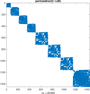
(a) C atom

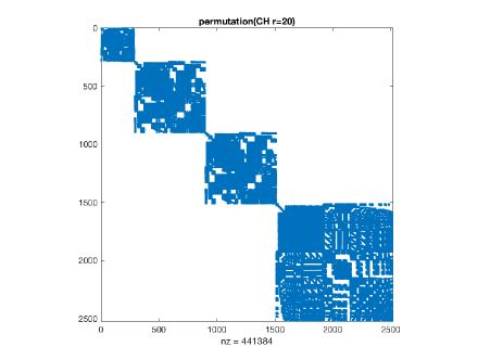
(b) CH molecule

Fig. 1: The block diagonal structures within the largest spin blocks of the $T_{2}$ matrices associated with the carbon (C) atom and the CH molecule.

In addition to exploiting the block diagonal structure in the $S_{j}$ matrices that appear in the dual SDP, we can also use the low rank structure of $\{X_{i}\}$ and $U$ to reduce the cost for solving (20). The following theorem shows that $\{X_{i}\}$, $i=1,2,...,l$ and $U$ in the primal (20) are indeed low rank as long as $d$ is sufficiently large.

Theorem 1.

Assume that there exists matrices $\hat{X}_{j}\succ 0$ and $\hat{U}\succ 0$ such that the linear equality constraints of (20) are satisfied with them and the basis size $d$ is larger than $3$. Then there exists an optimal solution $\{X_{1},\ldots,X_{l},U\}$ of (20) such that $r=\sum_{j=1}^{l}r_{j}+r_{u}\leq\frac{\sqrt{3}}{8}(d^{2}+6)$, where $r_{j}$ is the rank of $X_{j}$ and $r_{u}$ is the rank of $U$. Moreover, $r_{j}/s_{j}=O(1/d)$ for $j$’s associated with the T1, T2 and T2’ conditions.

Proof.

We first prove that there must exist a solution such that $r\leq\sqrt{m}$, where $m$ is the length of the dual variable $y$ in (19). The primal SDP (20) can be written as a standard SDP in the form of (21), where $X$ is a block diagonal matrix whose diagonal parts are $U$, $X_{j}$ and $\mathop{\operator@font diag}\nolimits(x)$. Then the size of $X$ is $\sum_{j=1}^{l}s_{j}+s_{u}+2s$. Let the rank of $X$ be $\tilde{r}$. It follows from the results shown in [23] that $\frac{\tilde{r}(\tilde{r}+1)}{2}\leq m$, which implies $\sum_{j=1}^{l}s_{j}+s_{u}+2s\leq\sqrt{m}$. Since $m=\frac{3}{64}d^{4}-\frac{1}{16}d^{3}+\frac{9}{16}d^{2}+\frac{1}{4}d\leq(\frac{\sqrt{3}}{8}(d^{2}+6))^{2}$ when $d\geq 3$, the first statement holds. The second statement follows from Table 1 that the dimension of the $S_{j}$ matrices associated with the T1, T2, T2’ conditions are on the order of $O(d^{3})$. ∎

3 The ADMM and DRS method

We now discuss using first-order methods to solve the SDP formulations of the ground state energy minimization problem for a many-electron system. For simplicity, let us first consider a generic SDP problem. Given $C,X\in\mathbb{R}^{n\times n}$, we define the linear operator $\mathcal{A}:\mathbb{R}^{n\times n}\rightarrow\mathbb{R}^{m}$ by $\mathcal{A}X=(\left\langle{A_{1}},{X}\right\rangle,\cdots,\left\langle{A_{m}},{X}\right\rangle)^{T}$ where $A_{1},\cdots,A_{m}\in\mathbb{R}^{n\times n}$. The conjugate operator of $\mathcal{A}$ is defined by $\mathcal{A}^{*}y=\sum_{p=1}^{m}A_{p}y_{p}$ for $y\in\mathbb{R}^{m}$. Using these notation, we can formulate a primal SDP as

(21) $$\max_{X} \left\langle{C},{X}\right\rangle$$

 s.t. $$\mathcal{A}X=b,$$

$$X\succeq 0.$$

The corresponding dual SDP is

(22) $$\begin{split}\min_{y,S}\ &b^{T}y\\ \,\textrm{s.t.}\,\ &S=\mathcal{A}^{*}y-C,\\ &S\succeq 0.\\ \end{split}$$

3.1 The DRS method

The DRS method, first introduced to solve nonlinear partial differential equations [8, 15, 10], can be used to solve the primal SDP. To describe the DRS method, we first establish some notations and terminologies. Given a convex function $f$ and a scalar $t>0$, the proximal mapping of $f$ is defined by

(23) $$\mathbf{prox}_{tf}(X):=\operatorname*{arg\,min}\limits_{U}f(U)+\frac{1}{2t}\|U-X\|_{F}^{2}.$$

We also define an indicator function on a convex set $\Omega$ as

$$1_{\Omega}(X):=\begin{cases}0,&\mbox{ if }X\in\Omega,\\ +\infty,&\mbox{ otherwise}.\end{cases}$$

To use the DRS method to solve (21), we let

(24) $$f(X)=-\left\langle{C},{X}\right\rangle+1_{\{\mathcal{A}X=b\}}(X)\mbox{ and }h(X)=1_{K}(X),$$

where $K=\{X:X\succeq 0\}$. Then each iteration of the DRS procedure for solving (21) can be described by the following sequences of steps

(25) $$\begin{split}&X^{k+1}=\mathbf{prox}_{th}(Z^{k}),\\ &U^{k+1}=\mathbf{prox}_{tf}(2X^{k+1}-Z^{k}),\\ &Z^{k+1}=Z^{k}+U^{k+1}-X^{k+1},\end{split}$$

where $\{U^{k}\}$ and $\{Z^{k}\}$ are two sets of auxiliary variables. It follows from some simple algebraic rearrangements that the variables $X$ and $U$ can be eliminated in (25) to yield a fixed-point iteration of the form

(26) $$Z^{k+1}=T_{\textrm{DRS}}(Z^{k}),$$

where

(27) $$T_{\textrm{DRS}}:=I+\mathbf{prox}_{tf}\circ(2\mathbf{prox}_{th}-I)-\mathbf{prox}_{th}.$$

3.2 ADMM

The ADMM is another method for solving the dual formulation of the SDP  (22). Let $X$ be the Lagrangian multiplier associated with the linear equality constraints of (22). The augmented Lagrangian function is

$$L_{\mu}(y,S,X)=b^{T}y+\left\langle{X},{S-\mathcal{A}^{*}y+C}\right\rangle+\frac{\mu}{2}||S-\mathcal{A}^{*}y+C||_{F}^{2}.$$

Applying ADMM [33] to (22) yields the following sequence of steps in the $k$th iteration

(28) $$\begin{split}&y^{k+1}={\arg\min}_{y}L_{\mu}(y,S^{k};X^{k}),\\ &S^{k+1}={\arg\min}_{S\succeq 0}L_{\mu}(y^{k+1},S;X^{k}),\\ &X^{k+1}=X^{k}+\mu(S^{k+1}-\mathcal{A}^{*}y^{k+1}+C).\\ \end{split}$$

In practice, the penalty parameter $\mu$ is often updated adaptively to achieve faster convergence in the ADMM. One strategy is to tune $\mu$ to balance the primal infeasibility $\eta_{p}$ and the dual infeasibility $\eta_{d}$ defined by

(29) $$\eta_{p}=\frac{\|\mathcal{A}(X)-b\|_{2}}{\max(1,\|b\|_{2})}\quad\text{and}\quad\eta_{d}=\frac{\|\mathcal{A}^{*}y-C-S\|_{F}}{\max(1,\|C\|_{F})}.$$

If the mean of $\eta_{p}/\eta_{q}$ in a few steps is larger (or smaller) than a constant $\delta$, we decrease (or increase) the penalty parameter $\mu$ by a multiplicative factor $\gamma$ (or $1/\gamma$) with $0<\gamma<1$. To prevent $\mu$ from becoming excessively large or small, a upper and lower bound are often imposed on $\mu$. This strategy has been demonstrated to be effectively in [33].

3.3 The connection between ADMM and DRS

It is well known that the DRS for the primal (21) is equivalent to the ADMM for dual (22). In particular, the $X$ variable produced in the $k$th step of DRS applied to (21) is exactly the $X$ variable produced in the $k$th step of ADMM applied to (22). The other variables ($Z$ and $U$) and the parameter $t$ produced in DRS are related to the variables $y$, $S$ and parameter $\mu$ produced in the ADMM via

(30) $$\left\{\begin{split}t&=\mu;\\ Z^{k}&=X^{k}-t\mathcal{A}^{*}y^{k};\\ U^{k}&=X^{k-1}+t(\mathcal{A}^{*}y^{k-1}+S^{k}-C).\end{split}\right.$$

If the DRS (25) is first executed, we can obtain the following relationship for the ADMM as

(31) $$\left\{\begin{split}t&=\mu;\\ X^{k}&=\mathbf{prox}_{th}(Z^{k-1});\\ S^{k}&=\frac{1}{t}(X^{k}-Z^{k});\\ \mathcal{A}^{*}y^{k}&=\frac{1}{t}(X^{k}-X^{k-1})-S^{k}+C.\end{split}\right.$$

The variable $y^{k}$ can be further computed from the last equation if the operator $\mathcal{A}$ is of full row rank. Consequently, the strategies of the ADMM for updating $\mu$ can be used in the DRS for modifying $t$ and vice versa. However, one should be careful on computing the primal and dual infeasibilities of the DRS when the parameter $t$ is changed from $t_{1}$ to $t_{2}$ after one loop of the DRS (25). In this case, the next immediate update of the DRS should be

(32) $$\begin{split}&X^{k+1}=\mathbf{prox}_{t_{1}h}\left(Z^{k}\right),\\ &U^{k+1}=\mathbf{prox}_{t_{2}f}\left(X^{k+1}-\frac{t_{2}}{t_{1}}(Z^{k}-X^{k+1})\right),\\ &Z^{k+1}=\frac{t_{2}}{t_{1}}(Z^{k}-X^{k+1})+U^{k+1}.\\ \end{split}$$

Thereafter, the original iterations (25) can still be used for the fixed $t_{2}$.

3.4 Application to the 2-RDM

The ADMM has been successfully used to solve the 2-RDM problem in [19] where the method is refereed to as the boundary point method. To apply ADMM to solve  (19), we first write the augmented Lagrangian function as

(33) $$\begin{split}L(y,S_{j};X_{j},x)&=b^{T}y+\sum_{j=1}^{l}\left\langle{X_{j}},{S_{j}-\mathcal{A}_{j}^{*}y+C_{j}}\right\rangle+\left\langle{x},{c-B^{T}y}\right\rangle\\ &+\frac{\mu}{2}(\sum_{j=1}^{l}\|S_{j}-\mathcal{A}_{j}^{*}y+C_{j}\|_{F}^{2}+\|c-B^{T}y\|_{2}^{2}),\end{split}$$

where $X_{j}$ and $x$ are Lagrangian multipliers and $\mu>0$ is a penalty parameter. The the $k$th iteration of ADMM consists of the following sequence of steps:

(34) $$\begin{split}&y^{k+1}={\arg\min}_{y}L(y,S_{j}^{k};X_{j}^{k},x^{k}),\\ &S_{1}^{k+1}={\arg\min}_{0\preceq S_{1}\preceq I}L(y^{k+1},S_{j};X_{j}^{k},x^{k}),\\ &S_{j}^{k+1}={\arg\min}_{S_{j}\succeq 0}L(y^{k+1},S_{j};X_{j}^{k},x^{k}),\ j=2,\cdots,l,\\ &X_{j}^{k+1}=X_{j}^{k}+\mu(S_{j}^{k+1}-\mathcal{A}_{j}^{*}y^{k+1}+C_{j}),\ j=1,\cdots,l,\\ &x^{k+1}=x^{k}+\mu(c^{k+1}-B^{T}y^{k+1}).\end{split}$$

The convergence of ADMM has been studied in [12, 9, 2, 5, 33]. The following theorem, which establish the convergence of the ADMM to the solution of (19) follows from the analysis given in [33, Theorem 2.9].

Theorem 2.

Suppose that the KKT points of (19) exist. Then the sequence of variables $(X_{j}^{k},x^{k},S_{j}^{k},y^{k})$ generated from the ADMM converge to a solution $(X_{j}^{*},x^{*},S_{j}^{*},y^{*})$ of (19) from any starting point. Furthermore, $\|\sum_{j=1}^{l}\left\langle{X_{j}^{k}},{C_{j}}\right\rangle+c^{T}x-b^{T}y^{k}\|$, $\|\sum_{j=1}^{l}\mathcal{A}_{j}X_{j}+Bx-b\|$, $\|\mathcal{A}_{j}^{*}y^{k}-C-S_{j}^{k}\|_{F}$ and $\|B^{T}y^{k}-c\|$ all converge to 0.

4 The Semi-smooth Newton method

Although Theorem 2 asserts that the ADMM (and consequently the DRS method due to its equivalence to the ADMM) converges from any starting point, the convergence can be slow, especially towards a highly accurate approximation to the solution of (19). In practice, we often observe a rapid reduction in the objective function, infeasibility and duality gap in the first few iterations. However, the reduction levels off after the first tens or hundreds of iterations. To accelerate convergence and obtain a more accurate approximation, we consider a second-order method.

The DRS can be characterized as a fixed-point iteration (26) for solving a system of nonlinear equations

(35) $$F(Z)=\mathbf{prox}_{th}(Z)-\mathbf{prox}_{tf}(2\mathbf{prox}_{th}(Z)-Z)=0,$$

where $Z\in\mathbb{R}^{n\times n}$. Moreover, the solution of (35) is also an optimal solution to (21) and vice versa. Hence, we will focus on more efficient ways to solve the equations (35). To simplify the derivation of the new method to be presented, we first make the following assumption.

Assumption 3.

The operator $\mathcal{A}$ in (21) satisfies $\mathcal{A}\mathcal{A}^{*}=I$ and the Slater condition holds. That is, there exits $X\succ 0$ such that $\mathcal{A}X=b$.

The first part of the assumption implies that $\mathcal{A}$ has full row rank. It is satisfied in many SDPs including (19) after a suitable transformation of $\mathcal{A}$.

4.1 Generalized Jacobian

Before we discuss how to solve (35), let us first examine the structure of the generalized Jacobian of $F(Z)$. Using the definition of $f(x)$ and $h(x)$ given in (24), we can write down the explicit forms of $\mathbf{prox}_{tf}(Y)$ and $\mathbf{prox}_{th}(Z)$ as

$$\mathbf{prox}_{tf}(Y) = (Y+tC)-\mathcal{A}^{*}(\mathcal{A}Y+t\mathcal{A}C-b),$$

$$\mathbf{prox}_{th}(Z) = Q_{\dagger}\Sigma_{+}Q_{\dagger}^{T},$$

and where

$$Q\Sigma Q^{T}=\begin{pmatrix}Q_{\dagger}&Q_{\ddagger}\end{pmatrix}\begin{pmatrix}\Sigma_{+}&0\\ 0&\Sigma_{-}\end{pmatrix}\begin{pmatrix}Q_{\dagger}^{T}\\ Q_{\ddagger}^{T}\end{pmatrix}$$

is the spectral decomposition of the matrix $Z$, and the diagonal matrices $\Sigma_{+}$ and $\Sigma_{-}$ contain the nonnegative and negative eigenvalues of $Z$.

Although $F$ is not differentiable, its generalized subdifferential still exists. Since $F$ is locally Lipschitz continuous, it can be verified that $F$ is almost differentiable everywhere. We next introduce the concepts of generalized subdifferential.

Definition 4.

Let $F$ be locally Lipschitz continuous at $X\in{\mathcal{O}}$, where ${\mathcal{O}}$ is an open set. Let $D_{F}$ be the set of differentiable points of $F$ in ${\mathcal{O}}$. The B-subdifferential of $F$ at $X$ is defined by

$$\partial_{B}F(X):=\left\{\lim\limits_{k\rightarrow\infty}F^{\prime}(X^{k})|X^{k}\in D_{F},X^{k}\rightarrow X\right\}.$$

The set $\partial F(x)=\emph{co}(\partial_{B}F(x))$ is called Clarke’s generalized Jacobian, where co denotes the convex hull.

It can be shown that the generalized Jacobian matrix associated with the second term of $F(Z)$ in (35) has the form

(36) $$\mathcal{D}\equiv\partial\mathbf{prox}_{tf}((2\mathbf{prox}_{th}(Z)-Z))=\mathcal{I}-\mathcal{A}^{*}\mathcal{A},$$

where $\mathcal{I}$ is the identity operator. Similar to the convention used in [36], we define a generalized Jacobian operator $\mathcal{M}(Z)\in\partial\mathbf{prox}_{th}(Z)$ in terms of its application to an $n$-by-$n$ matrix $S$ that yields

(37) $$\mathcal{M}(Z)[S]=Q(\Omega\circ(Q^{T}SQ))Q^{T},\forall S\succeq 0,$$

where $Q\Sigma Q^{T}$ is the eigen-decomposition of $Z$ with $\Sigma=\mathop{\operator@font diag}\nolimits(\lambda_{1},\cdots,\lambda_{n})$, and

$$\Omega=\left[\begin{matrix}E_{\alpha\alpha}&k_{\alpha\bar{\alpha}}\\ k_{\alpha\bar{\alpha}}^{T}&0\end{matrix}\right],$$

with $\alpha=\{i|\lambda_{i}>0\}$, $\bar{\alpha}=\{1,\ldots,n\}\setminus\alpha$ and $E_{\alpha\alpha}$ being a matrix of ones and $k_{ij}=\frac{\lambda_{i}}{\lambda_{i}-\lambda_{j}},i\in\alpha,j\in\bar{\alpha}.$ The $\circ$ symbol appeared in (37) denotes a Hadamard product. It follows from (35), (36) and (37) that the generalized Jacobian of $F(z)$ can be written as

(38) $$\mathcal{J}(Z)=\mathcal{M}(Z)+\mathcal{D}(I-2\mathcal{M}(Z)).$$

The function $F$ given in (35) is strongly semi-smooth [20, 24] and monotone, which is important for establishing the positive semidefinite nature of its $B$-subdifferential. The precise definitions of these properties are given below.

Definition 5.

Let $F$ be a locally Lipschitz continuous function in a domain ${\mathcal{O}}$. We say that $F$ is semi-smooth at $x\in{\mathcal{O}}$ if (i) $F$ is directionally differentiable at $x$; (ii) for any $z\in{\mathcal{O}}$ and $\mathcal{J}\in\partial F(x+z)$,

(39) $$\|F(x+z)-F(x)-\mathcal{J}[z]\|_{2}=o(\|z\|_{2})\quad\mbox{as}\ z\rightarrow 0.$$

The function $F$ is said to be strongly semi-smooth if $o(\|z\|_{2})$ in (39) is replaced by $O(\|z\|_{2}^{2})$. It is called monotone if $\left\langle{x-y},{F(x)-F(y)}\right\rangle\geq 0,\ \mbox{for all}\ x,y\in\mathbb{R}^{n}$.

The next lemma characterizes the fixed point map given in (35) and its generalized Jacobian matrix.

Lemma 6.

The function $F$ in (35) is strongly semi-smooth and monotone. Each element of B-subdifferential $\partial_{B}F(x)$ of $F$ is positive semidefinite.

Proof.

The strongly semi-smoothness of $F$ follows from the derivation given in [25, 29] to establish the semi-smoothness of proximal mappings. In fact, the projection over a polyhedral set is strongly semi-smooth [25, Example 12.31] and the projections over symmetric cones are proved to be strongly semi-smooth in [29]. Hence, $\mathbf{prox}_{tf}(\cdot)$ and $\mathbf{prox}_{th}(\cdot)$ are strongly semi-smooth. Since strongly semi-smoothness is closed under scalar multiplication, summation and composition, the function $F$ is strongly semi-smooth.

It has been shown in [15] that the operator $T_{\textrm{DRS}}$ is firmly nonexpansive. Therefore, $F$ is firmly nonexpansive, hence monotone [1, Proposition 4.2]. The positive semidefiniteness simply follows from Lemma 3.5 in [34]. ∎

4.2 Computing the Newton direction

Using the expression given in (38), we can now discuss how to compute the Newton direction efficiently. At a given iterate $Z^{k}$, we compute a Newton direction $S^{k}$ by solving the equation

(40) $$(\mathcal{J}_{k}+\mu_{k}\mathcal{I})[S^{k}]=-F^{k},$$

where $\mathcal{J}_{k}\in\partial_{B}F(Z^{k})$, $F^{k}=F(Z^{k})$, $\mu_{k}=\lambda_{k}\|F^{k}\|_{2}$ and $\lambda_{k}>0$ is a regularization parameter. The equation (40) is well-defined since each element of B-subdifferential $\partial_{B}F(x)$ of $F$ is positive semidefinite and the regularization term $\mu_{k}I$ is chosen such that $\mathcal{J}_{k}+\mu_{k}\mathcal{I}$ is invertible. From a computational view, it is not practical to solve the linear system (40) exactly. Therefore, we seek an approximate step $S^{k}$ by solving (40) approximately so that

(41) $$\|r^{k}\|_{F}\leq\tau\min\{1,\lambda_{k}\|F^{k}\|_{F}\|S^{k}\|_{F}\},$$

where

(42) $$r^{k}:=(\mathcal{J}_{k}+\mu_{k}\mathcal{I})[S^{k}]+F^{k}$$

is the residual and $0<\tau<1$ is some positive constant.

Since the $\mathcal{J}_{k}$ matrix in (40) is nonsymmetric, and its dimension is large, we apply the binomial inverse theorem to transform (40) into a smaller symmetric system. If we vectorize the matrix $S$, then the operators $\mathcal{M}(Z)$ and $\mathcal{D}$ can be expressed as matrices

$$M(Z)=\tilde{Q}\Lambda\tilde{Q}^{T}\ \text{and}\ D=I-A^{T}A，$$

respectively, where $\tilde{Q}=Q\otimes Q$, $\Lambda=\mathop{\operator@font diag}\nolimits(\mathrm{vec}(\Omega))$, $I$ is the identity matrix and $A$ is the matrix form of $\mathcal{A}$. Let $W=I-2M(Z)=\tilde{Q}(I-2\Lambda)\tilde{Q}^{T}$ and $H=\tilde{Q}((\mu_{k}+1)I-\Lambda)\tilde{Q}^{T}$. Then the matrix form of $\mathcal{J}_{k}+\mu_{k}I$ can be written as $J_{k}+\mu_{k}I=H-A^{T}AW$. It follows from the binomial inverse theorem that

$$(J_{k}+\mu_{k}I)^{-1} = (H-A^{T}AW)^{-1}$$

$$= H^{-1}+H^{-1}A^{T}(I-AWH^{-1}A^{T})^{-1}AWH^{-1}.$$

Define

(43) $$T=\tilde{Q}L\tilde{Q}^{T},$$

where $L$ is a diagonal matrix with diagonal entries $L_{ii}=\frac{\Lambda_{ii}\mu_{k}}{\mu_{k}+1-\Lambda_{ii}}$. By using the identities $H^{-1}=\frac{1}{\mu_{k}+1}I+\frac{1}{\mu_{k}(\mu_{k}+1)}T$ and $WH^{-1}=\frac{1}{1+\mu_{k}}I-(\frac{1}{\mu_{k}}+\frac{1}{\mu_{k}+1})T$, we can further obtain

$$(J_{k}+\mu_{k}I)^{-1}$$

$$= \frac{\mu_{k}I+T}{\mu_{k}(\mu_{k}+1)}\left(I+A^{T}\left(\frac{\mu_{k}^{2}}{2\mu_{k}+1}I+ATA^{T}\right)^{-1}A(\frac{\mu_{k}}{2\mu_{k}+1}I-T)\right).$$

As a result, the solution of (40) can be obtained by first solving the following symmetric linear equation

(45) $$\left(\frac{\mu_{k}^{2}}{2\mu_{k}+1}I+ATA^{T}\right)d_{s}=a,$$

where $a=-A(\frac{\mu_{k}}{2\mu_{k}+1}I-T)\mathrm{svec}(F^{k})$, by an iterative method such as the conjugate gradient (CG) method or the symmetric QMR method. Note that the size of the coefficient matrix of (45) is $m\times m$ while that of (40) is $n^{2}\times n^{2}$, where $m$ usually is much smaller than $n^{2}$. Then we use the following expression to recover

$$S^{k}=\frac{1}{\mu_{k}(\mu_{k}+1)}(\mu_{k}\mathcal{I}+\mathcal{T})[-F^{k}+\mathcal{A}^{*}d_{s}],$$

where $\mathcal{T}$ is the operator form of $T$ in (43). Specifically, applying $\mathcal{T}$ to a matrix $S$ yields

$$\mathcal{T}(Z)[S]=Q(\Omega_{0}\circ(Q^{T}SQ))Q^{T},\forall S\succeq 0,$$

where $\Omega_{0}=\left[\begin{matrix}E_{\alpha\alpha}&l_{\alpha\bar{\alpha}}\\ l_{\alpha\bar{\alpha}}^{T}&0\end{matrix}\right]$, and $l_{ij}=\frac{\mu_{k}k_{ij}}{\mu_{k}+1-k_{ij}}$.

Let $\Upsilon=\mathcal{T}(Z)[S]$. We can then use the same techniques used in [36] to express $\Upsilon$ as multiplication:

(46) $$\Upsilon=[Q_{\alpha}Q_{\bar{\alpha}}]\left[\begin{matrix}Q_{\alpha}^{T}SQ_{\alpha}&l_{\alpha\bar{\alpha}}\circ Q_{\alpha}^{T}SQ_{\bar{\alpha}}\\ l_{\alpha\bar{\alpha}}^{T}\circ Q_{\bar{\alpha}}^{T}SQ_{\alpha}&0\end{matrix}\right]\left[\begin{matrix}Q_{\alpha}^{T}\\ Q_{\bar{\alpha}}^{T}\end{matrix}\right]=G+G^{T},$$

where $G=Q_{\alpha}(\frac{1}{2}(UQ_{\alpha}^{T})+l_{\alpha\bar{\alpha}}\circ(UQ_{\bar{\alpha}}))$ with $U=Q_{\alpha}^{T}S$. The number of floating point operations (flops) required to compute $\Upsilon$ is $8|\alpha|n^{2}$. If $|\alpha|$ is large, we can compute $\Upsilon$ via the equivalent expression $\Upsilon=S-Q((E-\Omega_{0})\circ(Q^{T}SQ))Q^{T}$, which requires $8|\bar{\alpha}|n^{2}$ flops.

Therefore, using the expression (46) allow us to obtain an approximate solution to (40) efficiently whenever $|\alpha|$ or $|\bar{\alpha}|$ is small. We summarize the procedure for solving the Newton equation (40) approximately in Algorithm 1.

1 Compute $a=-\mathcal{A}(\frac{\mu_{k}}{2\mu_{k}+1}\mathcal{I}-\mathcal{T})F^{k}$ ;

2 Use the CG or symmetric QMR method to solve $(\frac{\mu_{k}^{2}}{2\mu_{k}+1}\mathcal{I}+\mathcal{A}\mathcal{T}\mathcal{A}^{*})d_{s}=a$ inexactly, where the matrix-vector multiplication is computed by (46) ;

Compute the Newton direction $S^{k}=\frac{1}{\mu_{k}(\mu_{k}+1)}(\mu_{k}\mathcal{I}+\mathcal{T})(-F^{k}+\mathcal{A}^{*}d_{s})$.

Algorithm 1 Solving the linear system (40)

4.3 Strategy for updating $Z^{k}$

A few safeguard strategies are developed in order to stabilize the semi-smooth Newton algorithm and maintain global convergence. Let $U^{k}=Z^{k}+S^{k}$ be a new trial point from the Newton step and set $\xi_{0}=\|F(Z^{0})\|_{2}$. If the residual $\|F(U^{k})\|$ is sufficiently decreased, i.e., $\|F(U^{k})\|_{2}\leq\nu\xi_{k}$ with $0<\nu<1$, then we update

(47) $$Z^{k+1}=U^{k},\;\xi_{k+1}=\|F(U^{k})\|_{2}\mbox{ and }\lambda_{k+1}=\lambda_{k}.$$

Otherwise, we examine the ratio

(48) $$\rho_{k}=\frac{-\left\langle{F(U^{k})},{S^{k}}\right\rangle}{\|S^{k}\|_{F}^{2}}$$

to decide how to update $Z^{k}$, $\xi_{k}$ and $\lambda_{k}$. If $\rho_{k}\geq\eta_{1}$ for some $\eta_{1}$ that satisfies $0<\eta_{1}\leq\eta_{2}<1$, we compute a new trial point using so-called hyperplane projection step [28]:

(49) $$V^{k}=Z^{k}-\frac{\left\langle{F(U^{k})},{Z^{k}-U^{k}}\right\rangle}{\|F(U^{k})\|_{2}^{2}}F(U^{k}).$$

Assume that the set of the optimal solutions of (35) is $\Omega$. By the monotonicity of $F$, for any optimal solution $Z^{*}$, one always has $\left\langle{F(U^{k})},{Z^{*}-U^{k}}\right\rangle\leq 0$. If the ratio $\rho_{k}>0$, then we have $\left\langle{F(U^{k})},{-S^{k}}\right\rangle>0$. Therefore, the hyperplane

$$H_{k}:=\{Z\in\mathbb{R}^{n\times n}|\left\langle{F(U^{k})},{Z-U^{k}}\right\rangle=0\}$$

strictly separates $Z^{k}$ from the solution set $\Omega$. It is easy to show that the point $V^{k}$ defined in (49) is the projection of $Z^{k}$ onto the hyperplane $H_{k}$ and it is closer to $Z^{*}$ than $Z^{k}$. This projection step can be used to correct a potentially poor Newton step. Hence, we set $Z^{k+1}=V^{k}$ if $\|F(V^{k})\|_{2}\leq\|F(Z^{k})\|_{2}$. Otherwise, we still take a DRS iteration, i.e., $W^{k}=Z^{k}-F(Z^{k})$. In summary, we set

(50) $$Z^{k+1}=\begin{cases}V^{k},\ &\textrm{if}\;\rho_{k}\geq\eta_{1}\;\mbox{and}\;\|F(V^{k})\|_{2}\leq\|F(Z^{k})\|_{2},\;\mbox{ [projection step]}\\ W^{k},&\textrm{if}\;\rho_{k}\geq\eta_{1}\;\mbox{and}\;\|F(V^{k})\|_{2}>\|F(Z^{k})\|_{2},\;\mbox{ [DRS step]}\\ Z^{k},&\textrm{if}\;\rho_{k}<\eta_{1},\qquad\qquad\qquad\qquad\qquad\quad\quad\mbox{ [unsuccessful step]}\end{cases}$$

Then the parameters $\xi_{k+1}$ and $\lambda_{k+1}$ are updated as

(51) $$\xi_{k+1}=\xi_{k},\quad\lambda_{k+1}\in\begin{cases}(\uline{\lambda},\lambda_{k}),&\textrm{if}\ \rho_{k}\geq\eta_{2},\\[8.0pt] [\lambda_{k},\gamma_{1}\lambda_{k}],&\textrm{if}\ \eta_{1}\leq\rho_{k}<\eta_{2},\\[8.0pt] (\gamma_{1}\lambda_{k},\gamma_{2}\lambda_{k}],&\textrm{otherwise,}\end{cases}$$

where $1<\gamma_{1}<\gamma_{2}$ and $\uline{\lambda}>0$ is a small positive constant.

The complete approach to solve (35) is summarized in Algorithm 2.

1 Give $0<\tau,\nu<1$, $0<\eta_{1}\leq\eta_{2}<1$ and $1<\gamma_{1}\leq\gamma_{2}$ ;

2 Choose $Z^{0}$ and $\varepsilon>0$. Set $k=0$ and $\xi_{0}=\|F(Z^{0})\|_{2}$;

3 while not “converged” do

4       Select $J_{k}\in\partial_{B}F(Z^{k})$;

5       Solve the linear system (40) approximately such that $S^{k}$ satisfies (41);

6       Compute $U^{k}=Z^{k}+S^{k}$ and calculate the ratio $\rho_{k}$ as in (48);

7       If $\|F(U^{k})\|_{2}\leq\nu\xi_{k}$, Set update $Z^{k+1}$, $\xi_{k+1}$ and $\lambda_{k+1}$ according to (47). Otherwise, set them according to (50) and (51), respectively;

8       Set $k=k+1$;

9      

Algorithm 2 An Adaptive Semi-smooth Newton (ASSN) method for SDP

The following theorem establishes the global convergence of Algorithm 2.

Theorem 7.

Suppose that $\{Z_{k}\}$ is a sequence generated by Algorithm 2. Then the residuals of $\{Z_{k}\}$ converge to 0, i.e., $\lim_{k\rightarrow\infty}||F(Z_{k})||=0$.

Proof.

The strongly semi-smoothness and monotonicity has been shown in Lemma 6 and the firmly non-expansiveness of fixed-point mapping $T_{\mathrm{DRS}}=I-F$ has been shown in [15]. The proof is completed according to Theorem 3.10 in [34]. ∎

5 Numerical Results

In this section, we demonstrate the effectiveness of the semi-smooth Newton method presented in the previous section. We implemented the algorithm mostly in MATLAB. Our codes are built based on +SDPNAL [36], SDPNAL+ [4] and ADMM+ [30], and use most of the key implementation details and subroutines in these solvers. Some parts of the code are written in the C Language and interfaced with MATLAB through MEX-files. All experiments are performed on a single node of a PC cluster, where each node has two Intel Xeon 2.40GHz CPUs with 12 cores and 256GB RAM.

The test dataset is provided by Professor Maho Nakata and Professor Mituhiro Fukuta. The detailed information about the dataset such as the basis sets used to discretize molecular orbitals, the geometries of the molecules etc. can be found in [21]. Since the original dataset only takes into account the spin symmetry, it does not specify additional block diagonal structures introduced by spatial symmetry of the molecular orbitals within each spin matrix block of the variables. We preprocess the dataset to identify these diagonal blocks automatically through matrix reordering. Our solver takes advantage of these block diagonal structures to reduce the complexity of the computation as described in subsection 2.3. We applied the semi-smooth Newton algorithm to the SDP formulation of the 2-RDM minimization problem with four different groups of N-representability conditions labeled as PQG, PQGT1, PQGT1T2, PQGT1T2’. The letters and numbers in each label simply indicate the N-representability conditions included in the SDP constraints. For example, PQGT1T2’ means that the P, Q, G, T1, T2’ conditions are included.

We compare the semi-smooth Newton’s method proposed in this paper with the state-of-the-art Newton-CG augmented Lagrangian method implemented in the SDPNAL software package [36]. We choose to compare with SDPNAL instead of SDPNAL+ [4] because our test examples are in standard SDP forms for which SDPNAL works better than SDPNAL+ in our numerical experiments. The interior point methods are not included in the comparison because they usually performs worse than SDPNAL. The stopping rules and a number of parameters used in SDPNAL are set to their default values. We measure accuracy by examining four criteria: the primal infeasibility $\eta_{p}$ and the dual infeasibility $\eta_{q}$ that are defined by (29), the gap $\eta_{g}$ between the primal and dual objective functions

(52) $$\eta_{g}=\frac{|b^{T}y-\mathrm{tr}(C^{T}X)|}{\max(1,\mathrm{tr}(C^{T}X))},$$

and the difference between the 2-RDM energy and full CI energy defined by

(53) $$\mathrm{err}=b^{T}y-\mathrm{energy_{fullCI}},$$

where $\mathrm{energy_{fullCI}}$ values are taken from [21]. The last criterion is often used in quantum chemistry to assess the accuracy of an approximation model. It is used here to also assess the effectiveness in including additional N-representability conditions in the 2-RDM formulation of the ground state energy minimization problem. In the following tables, we use a short notation for the exponential form. For example, -4.8-3 means $-4.8\times 10^{-3}$.

We experimented with two versions of the semi-smooth Newton methods. The difference between these two versions is in the stopping rules and how the parameter $\mu$ is updated. The first version, which is called SSNSDPL, uses a stopping rule that is similar to the one used in SDPNAL. Specifically, in this version, the iterative procedure is terminated when $\eta_{p}<3\times 10^{-6}$ and $\eta_{d}<3\times 10^{-7}$ so that it can achieve higher accuracy than that produced by SDPNAL. The choice of these parameters makes SSNSDPL comparable to SDPNAL. Another version, which is called SSNSDPH, uses a more stringent stopping rule that requires $\eta_{p}<1\times 10^{-4}$ and $\eta_{d}<1\times 10^{-9}$. In this version, the primal infeasibility $\eta_{p}$ is allowed to be larger so that the algorithm converges more rapidly. The dual variables are required to be more accurate since we ultimately retrieve the desired 1-RDM and 2-RDM from the dual variables. This version can reach a “$\mathrm{err}$” level that is close to the one reported in [21]. In this version, we also make the penalty parameter $\mu$ larger so that the stopping rules can be easier satisfied.

In Table LABEL:tab:sp, we compare the performance of SSNSDPL when it is applied to the orginal dataset provided in [21] and our preprocessed data that identifies additional block diagonal structures through permutation. We can see that the CPU time can be reduced by at least a factor of three on most examples labeled with PQGT1T2 and PQGT1T2’. For $\mathrm{C}$ atom and $\mathrm{F^{-}}$ system that exhibit high spatial symmetry, the CPU time measured in seconds (the column labeled by t in Table LABEL:tab:sp) can be reduced by a factor of roughly six for SDP’s that include the PQGT1T2 and PQGT1T2’ conditions. These experiments illustrate the importance of exploiting spatial symmetry to identify block diagonal structures in the approximate solution and consequently reduce the computational cost significantly. For the problems that only include the PQG and PQGT1 conditions, the amount of improvement is less spectacular, because the sizes of the diagonal blocks in these examples are small. In fact, the larger the blocks in Table 1 is, the more significant effectiveness of the symmetry is. Thereafter, all experiments are performed on the preprocessed data.

Table 2: The comparison of the performance on the original and proprocessed SDPs. The number -4.8-3 means $-4.8\times 10^{-3}$

		preprocessed SDP						original SDP
system	condition	err	$\eta_{p}$	$\eta_{d}$	$\eta_{g}$	it	t	err	$\eta_{p}$	$\eta_{d}$	$\eta_{g}$	it	t
$\mathrm{C}$	PQG	-4.8-3	1.3-6	3.0-7	1.0-5	335	136	-4.7-3	3.2-7	2.7-7	9.8-6	163	82
$\mathrm{C}$	PQGT1	-3.8-3	5.9-7	2.9-7	7.4-6	217	129	-3.8-3	5.3-7	2.9-7	7.0-6	157	189
$\mathrm{C}$	PQGT1T2	-9.9-4	9.3-7	2.8-7	7.7-6	229	366	-9.5-4	1.1-6	3.0-7	6.5-6	219	1915
$\mathrm{C}$	PQGT1T2’	-5.4-4	1.2-6	3.0-7	7.7-6	226	361	-5.4-4	1.7-6	3.0-7	1.2-5	235	2051
$\mathrm{CH}$	PQG	-1.3-2	1.3-6	3.0-7	9.5-6	126	77	-1.3-2	2.1-6	2.0-7	8.2-6	196	167
$\mathrm{CH}$	PQGT1	-1.0-2	1.7-7	2.7-7	9.7-6	122	220	-1.0-2	9.7-7	2.7-7	8.5-6	118	446
$\mathrm{CH}$	PQGT1T2	-2.5-3	1.9-6	3.0-7	1.0-5	271	2008	-2.5-3	4.0-7	3.0-7	1.1-5	268	6351
$\mathrm{CH}$	PQGT1T2’	-1.1-3	5.1-7	2.9-7	9.9-6	294	2041	-1.1-3	3.9-7	2.9-7	9.6-6	282	6350
$\mathrm{F^{-}}$	PQG	-1.3-2	6.3-7	1.8-7	8.5-6	119	72	-1.2-2	1.6-6	1.1-7	1.3-5	113	106
$\mathrm{F^{-}}$	PQGT1	-9.2-3	1.9-6	2.6-7	1.3-5	144	211	-8.7-3	1.1-6	2.6-7	5.4-6	149	718
$\mathrm{F^{-}}$	PQGT1T2	-2.6-3	2.1-6	2.7-7	2.2-5	225	1325	-2.7-3	1.3-6	2.8-7	1.7-5	235	10735
$\mathrm{F^{-}}$	PQGT1T2’	-2.0-3	1.2-6	2.7-7	1.1-5	249	1359	-1.9-3	1.2-6	3.0-7	1.2-5	234	9485
$\mathrm{H_{2}O}$	PQG	-1.9-2	2.2-6	1.2-7	1.6-6	87	93	-1.9-2	1.3-6	1.0-7	2.3-6	92	126
$\mathrm{H_{2}O}$	PQGT1	-1.2-2	2.4-6	2.5-7	1.3-5	124	408	-1.2-2	2.3-7	2.9-7	1.3-5	126	1070
$\mathrm{H_{2}O}$	PQGT1T2	-2.9-3	3.3-7	2.9-7	1.5-5	316	6213	-2.9-3	2.6-6	2.9-7	1.7-5	289	19392
$\mathrm{H_{2}O}$	PQGT1T2’	-2.0-3	1.2-6	3.0-7	1.1-5	257	4679	-2.0-3	2.4-6	2.9-7	9.0-6	252	16339

In addition to identifying block diagonal structures in the N-representibility constraints, we can further improve the efficiency of SSNSDPL and SSNSDPH by taking advantage of the low rank structure of the variable matrices. Recall from Theorem 1 that the ratios of the rank of the $X_{j}$ matrix (denoted by $r_{j}$) associated with the T2 condition over the dimension of $X_{j}$ (denoted by $d_{j}$) should be bounded by $(\frac{\sqrt{3}}{8}(d^{2}+6))/(\frac{d^{2}}{8}(\frac{3d}{2}-1))$. For the C atom and CH molecule, $d$ is 20 and 24 respectively. Thus, at the solution the ratios should be bounded by 0.06 and 0.05, respectively. In Figure 2, we replace $r_{j}$ by the numerical rank computed from the eigenvalue decompositions of the $X_{j}$ variable and show the ratios for $j$’s that are associated with the four largest $d_{j}$’s at each DRS iteration. We observe that these ratios can be relatively high in the first few iterations. But they eventually become less than 0.1 after a few hundred iterations. This property is useful (46) in the DRS and the semi-smooth Newton methods. It follows from (31) that the $X$ variable is the projection of the $Z$ variable to semidefinite cone and $|\alpha|$ in (46) is equal to the rank of $X_{j}$ in the case of 2-RDM. Therefore, solving the Newton system (45) becomes much cheaper by using (46) when $|\alpha|$ is small.

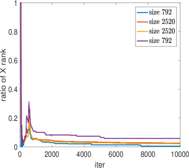
(a) C

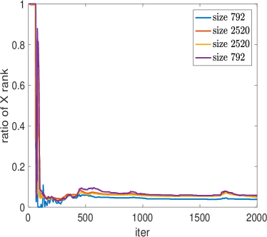
(b) CH

Fig. 2: The percentage of the ranks of the first four largest blocks of the $X$ in the C and CH systems

Figure 3 shows how the relative gap, primal infeasibility and dual infeasibility in ADMM and SSNSDPL change with respect to the number of iterations when they are applied to the C atom system. We tested both algorithms on SDPs with the PQG N-representibility conditions (shown in subfigures a and c) and with the PQGT1T2 N-representibility conditions (shown in subfigures b and d.) In subfigures (a) and (b), we show the convergence history of ADMM for the first 10000 steps. In subfigures (c) and (d), we show the convergence history of SSNSDPL. The starting points of SSNSDPL are taken to be the solution produced from running $500$ ADMM steps. We can see that the ADMM can produce a moderately accurate solution in a few hundred iterations from subfigures (a) and (b). At that point, convergence becomes slow. Many more iterations (10,000) are required to reach high accuracy. Using a starting point obtained from running 500 ADMM iterations, we can use SSNSDPL to obtain a more accurate solution in $250$ steps. Note that the duality gap as well as the primal and dual feasibility curves shown in (c) and (d) are highly oscillatory. The oscillation is due to the adaptive update of the penalty parameter $\mu$ for achieving a faster overall convergence rate. If the penalty parameter is held fixed, these curves become much smoother. But more iterations are needed to reach the desired accuracy.

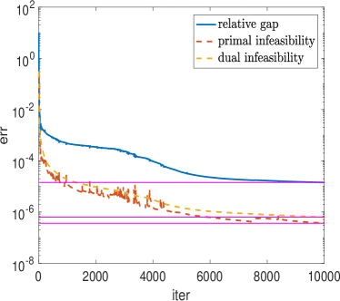
(a) ADMM on C(PQG)

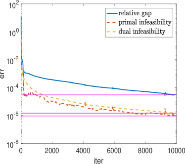
(b) ADMM on C(PQGT1T2)

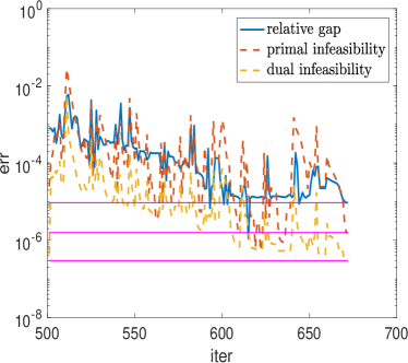
(c) SSNSDPL on C(PQG)

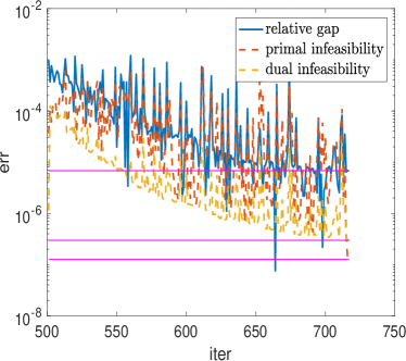
(d) SSNSDPL on C(PQGT1T2)

Fig. 3: Relative gap, primal infeasibility and dual infeasibility

The SSNSDPL and SSNSDPH methods have been successfully used to solve the SDPs with several types of N-representability conditions for all test problems. In Table LABEL:tab:err0, we report the accuracy of the solution produced by SSNSDPH by comparing the 2-RDM ground state energy with the FCI energy and calculating their differences defined by (53). We can see that more accurate solutions are obtained from SSNSDPH when more N-representability conditions are included in the constraints. These results are similar to the ones reported in  [21].

Table 3: The error obtained by SSNSDPH on various N-representability conditions: PQG, PQGT1, PQGT1T2, and PQGT1T2’

system	state	basis	PQG	PQGT1	PQGT1T2	PQGT1T2’
$\mathrm{AlH}$	1Sigma+	STO6G	-2.3-3	-7.8-4	-2.4-5	-1.4-5
$\mathrm{B_{2}}$	3Sigmag-	STO6G	-9.6-2	-8.5-2	-6.5-2	-6.4-2
$\mathrm{BF}$	1Sigma+	STO6G	-6.6-3	-3.5-3	-3.2-4	-3.1-4
$\mathrm{BH^{+}}$	2Sigma+	STO6G	-4.2-5	-2.6-5	-1.0-6	-2.9-7
$\mathrm{BH}$	1Sigma+	DZ	-6.5-3	-4.7-3	-8.6-5	-5.1-5
$\mathrm{BH_{3}O}$	1A1	STO6G	-2.8-2	-1.2-2	-7.1-4	-6.9-4
$\mathrm{BN}$	3Pi	STO6G	-2.9-2	-1.7-2	-3.0-3	-2.7-3
$\mathrm{BO}$	2Sigma+	STO6G	-1.2-2	-6.7-3	-1.2-3	-1.0-3
$\mathrm{Be(1)}$	1S	STO6G	-4.6-7	-4.8-7	-9.8-8	-1.2-7
$\mathrm{Be(2)}$	1S	SV	-5.8-5	-5.4-5	-1.8-6	-6.4-7
$\mathrm{BeF}$	2Sigma+	STO6G	-3.1-3	-1.7-3	-2.6-4	-1.9-4
$\mathrm{BeH^{+}}$	1Sigma+	STO6G	-2.4-5	-2.3-5	-2.5-7	-1.9-7
$\mathrm{BeH}$	2Sigma+	STO6G	-4.5-5	-2.2-5	-5.3-7	-2.5-7
$\mathrm{BeO}$	1Sigma+	STO6G	-1.3-2	-9.5-3	-1.7-3	-1.7-3
$\mathrm{C(1)}$	3P	DZ	-3.9-3	-3.1-3	-3.9-4	-5.1-5
$\mathrm{C(2)}$	3PSZ0	DZ	-1.7-2	-1.4-2	-2.4-3	-2.0-3
$\mathrm{C_{2}^{-}}$	2Sigmag+	STO6G	-2.6-2	-1.4-2	-2.4-3	-1.9-3
$\mathrm{C_{2}(1)}$	1Sigmag+	STO6G	-4.6-2	-2.5-2	-3.4-3	-3.5-3
$\mathrm{C_{2}(2)}$	1Sigmag+	VDZ	-5.4-2	-5.4-2	-3.2-3	-3.5-3
$\mathrm{CF}$	2Pir	STO6G	-7.7-3	-5.8-3	-6.2-4	-4.8-4
$\mathrm{CH}$	2Pir	DZ	-1.3-2	-9.6-3	-8.9-4	-3.1-4
$\mathrm{CH_{2}(1)}$	1A1	DZ	-1.9-2	-1.2-2	-3.9-4	-3.1-4
$\mathrm{CH_{2}(2)}$	3B1	DZ	4.1-1	4.2-1	4.3-1	4.3-1
$\mathrm{CH_{3}^{+}}$	1Ep	STO6G	-1.3-2	-3.8-3	-1.7-4	-1.6-4
$\mathrm{CH_{3}}$	2A2pp	VDZ	-1.7-2	-1.0-2	-9.4-4	-3.1-4
$\mathrm{CH_{3}N}$	1A1	STO6G	-3.9-2	-1.6-2	-1.0-3	-9.8-4
$\mathrm{CH_{4}}$	1A1	STO6G	-1.9-2	-4.1-3	-1.9-4	-1.8-4
$\mathrm{CN}$	2Sigma+	STO6G	-2.4-2	-1.2-2	-2.1-3	-1.7-3
$\mathrm{CO^{+}}$	2Sigma+	STO6G	-1.8-2	-9.2-3	-1.7-3	-1.4-3
$\mathrm{CO}$	1Sigma+	STO6G	-1.2-2	-7.2-3	-8.6-4	-8.6-4
$\mathrm{F^{-}}$	1S	DZ+d	-1.2-2	-7.6-3	-3.8-4	-2.7-4
$\mathrm{FH_{2}^{+}}$	1A1	STO6G	-1.1-3	-5.1-4	-1.7-5	-1.5-5
$\mathrm{H_{2}O}$	1A1	DZ	-1.9-2	-1.1-2	-4.9-4	-4.0-4
$\mathrm{H_{3}}$	2A1p	DZ	-7.7-4	-5.5-4	-1.6-6	-7.9-8
$\mathrm{HF}$	1Sigma+	DZ	-1.2-2	-5.8-3	-3.5-4	-2.7-4
$\mathrm{HLi_{2}}$	2A1	STO6G	-1.0-3	-6.6-4	-7.2-5	-1.0-5
$\mathrm{HN_{2}^{+}}$	1Sigma+	STO6G	-2.5-2	-1.1-2	-1.5-3	-1.5-3
$\mathrm{HNO}$	1Ap	STO6G	-1.9-2	-1.4-2	-8.9-4	-9.0-4
$\mathrm{Li}$	2S	STO6G	-3.3-8	-1.8-8	-1.7-8	-4.2-9
$\mathrm{Li_{2}}$	1Sigmag+	STO6G	-3.7-4	-2.9-4	-6.2-6	-4.3-6
$\mathrm{LiF}$	1Sigma+	STO6G	-1.6-3	-1.3-3	-2.5-4	-2.4-4
$\mathrm{LiH(1)}$	1Sigma+	DZ	-3.5-4	-2.0-4	-2.0-6	-6.7-7
$\mathrm{LiH(2)}$	1Sigma+	STO6G	-3.4-5	-2.5-5	-1.6-7	-9.3-8
$\mathrm{LiOH}$	1Sigma+	STO6G	-8.6-3	-4.0-3	-5.8-4	-5.7-4
$\mathrm{N}$	4S	DZ	-2.4-3	-9.0-4	-9.8-5	-1.1-5
$\mathrm{N_{2}^{+}}$	2Sigmag+	STO6G	-3.1-2	-1.6-2	-2.6-3	-2.2-3
$\mathrm{N_{2}}$	1Sigmag+	STO6G	-1.2-2	-8.8-3	-1.2-3	-1.2-3
$\mathrm{NH(1)}$	1Delta	DZ	-1.7-2	-1.3-2	-4.9-4	-4.5-4
$\mathrm{NH(2)}$	3Sigma-	DZ	-9.7-3	-5.2-3	-5.4-4	-1.4-4
$\mathrm{NH_{2}^{-}(1)}$	1A1	DZ	-2.4-2	-1.5-2	-6.5-4	-5.7-4
$\mathrm{NH_{2}^{-}(2)}$	1A1	STO6G	-2.0-3	-1.3-3	-2.2-5	-2.0-5
$\mathrm{NH_{3}^{+}}$	2A2pp	STO6G	-9.8-3	-1.8-3	-2.0-4	-1.1-4
$\mathrm{NH_{3}}$	1A1	VDZ	-2.3-2	-1.4-2	-5.0-4	-4.7-4
$\mathrm{NH_{4}^{+}}$	1A1	STO6G	-1.7-2	-4.2-3	-2.3-4	-2.2-4
$\mathrm{Na}$	2S	STO6G	-1.0-3	-4.9-4	-5.2-5	-3.9-5
$\mathrm{NaH}$	1Sigma+	STO6G	-3.5-3	-1.6-3	-8.3-5	-7.4-5
$\mathrm{Ne}$	1S	DZ	-6.7-3	-2.7-3	-2.3-4	-1.5-4
$\mathrm{O(1)}$	1D	DZ	-1.9-2	-1.4-2	-1.3-3	-1.2-3
$\mathrm{O(2)}$	3P	DZ	-1.2-2	-6.3-3	-6.9-4	-2.4-4
$\mathrm{O(3)}$	3PSZ0	DZ	-2.3-2	-1.9-2	-2.8-3	-1.6-3
$\mathrm{O_{2}^{+}}$	2Pig	STO6G	-1.7-2	-1.5-2	-2.4-3	-2.1-3
$\mathrm{P}$	4S	631G	-8.3-4	-3.0-4	-6.4-5	-7.3-6
$\mathrm{SiH_{4}}$	1A1	STO6G	-1.9-2	-3.6-3	-1.9-4	-1.6-4

In Table LABEL:tab:opt, we compare the accuracy and efficiency of SDPNAL, SSNSDPL and SSNSDPH. The fifth column labeled by “$\mathrm{itr}$” gives the total number of Newton systems that was solved. Therefore, it is meaningful to compare these columns. The column labeled by t gives the CPU time in seconds. From the table, we can observe that SSNSDPL and SDPNAL achieve the same level of accuracy. In terms of efficiency, SSNSDPL seems to be faster than SDPNAL for most examples. We ran SSNSDPH with a smaller $\eta_{d}$ than SSNSDPL. Hence, it produces more accurate energy values. Table LABEL:tab:opt shows that the errors of SSNSDPH is indeed smaller than SSNSDPL and they are similar to these in [21].

Table 4: A summary of computational results of SDPNAL, SSNSDPL and SSNSDPH.

	SDPNAL						SSNSDPL						SSNSDPH
id	err	$\eta_{p}$	$\eta_{d}$	$\eta_{g}$	itr	t	err	$\eta_{p}$	$\eta_{d}$	$\eta_{g}$	itr	t	err	$\eta_{p}$	$\eta_{d}$	$\eta_{g}$	itr	t
$\mathrm{AlH}$	-5.3-4	4.8-6	5.1-7	5.5-6	155	411	-3.6-4	8.4-7	3.0-7	1.2-6	84	305	-1.4-5	1.4-5	7.5-10	9.8-6	155	504
$\mathrm{B_{2}}$	-6.5-2	1.7-5	7.3-7	1.2-5	225	2260	-6.5-2	6.6-7	2.7-7	5.3-6	182	1938	-6.4-2	1.5-5	8.3-10	1.6-5	197	2152
$\mathrm{BF}$	-7.9-4	7.8-6	6.0-7	1.3-5	175	466	-7.0-4	2.1-6	2.7-7	3.7-6	134	433	-3.1-4	1.4-5	9.7-10	1.4-5	185	603
$\mathrm{BH^{+}}$	-1.2-4	2.4-6	7.1-7	2.8-6	192	86	-9.0-5	2.0-6	2.3-7	2.4-7	163	72	-2.9-7	1.0-5	9.8-10	4.8-6	245	102
$\mathrm{BH}$	-6.1-4	8.3-5	7.0-7	1.2-4	252	2004	-5.2-4	7.2-7	2.9-7	1.3-5	258	2151	-5.1-5	3.9-5	9.1-10	1.2-4	234	2105
$\mathrm{BH_{3}O}$	-1.7-3	1.1-5	6.9-7	1.7-5	183	4567	-1.6-3	1.3-6	2.9-7	1.7-6	99	3216	-6.9-4	7.4-6	9.7-10	1.1-5	205	5667
$\mathrm{BN}$	-3.3-3	2.2-5	7.2-7	1.9-5	214	494	-3.2-3	1.6-6	2.8-7	4.2-6	108	387	-2.7-3	1.3-5	1.0-9	1.9-5	246	723
$\mathrm{BO}$	-1.6-3	9.2-6	7.0-7	1.6-5	171	666	-1.5-3	2.9-6	2.9-7	1.8-6	88	490	-1.0-3	1.1-5	1.0-9	2.6-5	223	1069
$\mathrm{Be(1)}$	-4.7-5	2.2-7	9.5-7	1.5-6	116	19	-3.9-5	1.3-7	3.0-7	1.0-6	195	49	-1.2-7	9.2-6	4.1-10	1.5-6	227	54
$\mathrm{Be(2)}$	-1.6-4	7.4-5	7.1-7	6.0-6	221	249	-1.4-4	6.1-7	3.0-7	5.8-6	464	412	-6.4-7	1.3-5	9.9-10	3.3-7	313	327
$\mathrm{BeF}$	-6.6-4	1.2-5	6.6-7	1.8-5	177	482	-5.2-4	1.2-6	3.0-7	1.0-6	179	553	-1.9-4	9.4-6	9.9-10	1.1-5	187	608
$\mathrm{BeH^{+}}$	-7.3-5	9.1-6	5.6-7	4.5-6	198	95	-7.4-5	3.8-7	2.8-7	3.1-6	254	96	-1.9-7	1.2-5	9.9-10	1.7-6	217	87
$\mathrm{BeH}$	-8.5-5	6.4-6	7.6-7	4.7-6	201	91	-7.1-5	1.7-6	3.0-7	1.8-8	144	65	-2.5-7	1.8-5	9.5-10	9.1-7	229	101
$\mathrm{BeO}$	-2.2-3	1.3-5	7.2-7	2.3-5	199	495	-2.1-3	1.8-6	2.7-7	5.8-6	105	375	-1.7-3	6.4-6	9.7-10	1.4-5	220	695
$\mathrm{C(1)}$	-5.5-4	3.3-5	5.9-7	3.2-5	245	440	-5.4-4	1.2-6	3.0-7	7.7-6	226	361	-5.1-5	1.3-5	8.5-10	3.7-5	295	428
$\mathrm{C(2)}$	-2.6-3	1.5-5	6.5-7	1.3-5	233	424	-2.6-3	1.5-6	3.0-7	7.3-6	229	355	-2.0-3	1.2-5	9.2-10	2.4-5	230	386
$\mathrm{C_{2}^{-}}$	-2.4-3	7.0-6	6.1-7	1.4-5	175	319	-2.4-3	9.9-7	2.9-7	3.9-6	115	244	-1.9-3	9.6-6	9.0-10	1.9-5	235	418
$\mathrm{C_{2}(1)}$	-4.2-3	5.2-6	7.7-7	5.3-6	184	320	-4.1-3	9.6-7	3.0-7	3.3-6	112	241	-3.5-3	8.8-6	9.4-10	7.2-6	214	386
$\mathrm{C_{2}(2)}$	3.7-3	5.2-4	7.1-7	5.3-4	234	7291	-5.1-3	1.6-6	2.8-7	7.0-6	217	8381	-3.5-3	1.4-5	9.4-10	3.2-5	154	6858
$\mathrm{CF}$	-8.8-4	8.5-6	5.1-7	1.1-5	168	443	-8.1-4	1.4-6	2.9-7	2.1-6	115	437	-4.8-4	9.9-6	9.7-10	1.1-5	194	634
$\mathrm{CH}$	-1.1-3	9.3-5	6.4-7	1.1-4	234	1875	-1.1-3	5.1-7	2.9-7	9.9-6	294	2041	-3.1-4	1.9-5	1.0-9	5.6-5	272	2262
$\mathrm{CH_{2}(1)}$	-1.3-3	1.4-4	6.5-7	2.4-4	241	4834	-1.3-3	6.5-7	3.0-7	1.3-5	278	5870	-3.1-4	3.9-5	8.7-10	1.2-4	321	7671
$\mathrm{CH_{2}(2)}$	4.3-1	6.4-4	6.5-7	2.0-4	251	4383	4.3-1	9.7-7	2.9-7	1.3-5	327	7595	4.3-1	5.0-5	9.6-10	7.9-5	375	9245
$\mathrm{CH_{3}^{+}}$	-5.6-4	1.0-6	9.0-7	2.7-6	158	151	-4.5-4	6.7-7	2.3-7	1.7-6	135	133	-1.6-4	1.2-5	8.3-10	2.7-6	181	185
$\mathrm{CH_{3}}$	-1.4-3	3.3-5	7.8-7	5.0-5	203	7744	-1.2-3	1.5-6	3.0-7	8.8-6	265	6474	-3.1-4	1.1-5	8.7-10	1.7-5	212	6423
$\mathrm{CH_{3}N}$	-2.0-3	9.1-6	6.3-7	1.1-5	170	4100	-1.9-3	9.2-7	2.8-7	1.5-6	104	3160	-9.8-4	1.1-5	9.7-10	1.8-5	203	5250
$\mathrm{CH_{4}}$	-7.5-4	9.3-7	8.9-7	3.7-6	148	164	-6.0-4	3.8-7	2.6-7	2.9-6	109	155	-1.8-4	8.5-6	9.8-10	1.1-5	168	239
$\mathrm{CN}$	-2.2-3	1.2-5	5.4-7	2.0-5	185	461	-2.2-3	1.5-6	2.4-7	5.6-6	110	366	-1.7-3	9.1-6	1.0-9	1.9-5	277	724
$\mathrm{CO^{+}}$	-2.0-3	1.1-5	7.8-7	1.8-5	174	435	-2.0-3	1.8-6	2.9-7	4.7-6	118	357	-1.4-3	1.2-5	9.7-10	2.3-5	269	728
$\mathrm{CO}$	-1.3-3	1.3-5	6.8-7	1.9-5	162	408	-1.2-3	2.6-6	2.7-7	2.2-6	89	328	-8.6-4	9.7-6	9.8-10	1.7-5	204	638
$\mathrm{F^{-}}$	-2.0-3	8.8-5	5.2-7	1.5-4	238	1429	-2.0-3	1.2-6	2.7-7	1.1-5	249	1359	-2.7-4	2.0-5	8.5-10	7.8-5	282	1576
$\mathrm{FH_{2}^{+}}$	-2.3-4	1.2-6	6.4-7	2.2-6	146	99	-1.8-4	1.5-6	2.9-7	1.5-6	55	53	-1.5-5	1.1-5	9.9-10	2.0-6	178	153
$\mathrm{H_{2}O}$	-1.9-3	7.4-5	4.9-7	1.1-4	246	5704	-2.0-3	1.2-6	3.0-7	1.1-5	257	4679	-4.0-4	1.3-5	9.4-10	4.1-5	282	5928
$\mathrm{H_{3}}$	-3.3-5	8.5-7	9.7-7	7.5-6	143	51	-2.0-5	3.0-7	3.0-7	4.2-6	176	58	-7.9-8	5.7-6	9.8-10	8.4-6	204	80
$\mathrm{HF}$	-2.3-3	5.6-5	6.9-7	7.5-5	216	1745	-2.0-3	8.5-7	2.9-7	1.2-5	187	1438	-2.7-4	1.2-5	8.5-10	3.9-5	265	2038
$\mathrm{HLi_{2}}$	-2.8-4	1.9-5	7.7-7	2.2-5	240	1108	-1.9-4	2.0-6	2.9-7	6.9-6	447	1357	-1.0-5	3.0-5	8.8-10	2.3-5	168	755
$\mathrm{HN_{2}^{+}}$	-2.2-3	8.4-6	7.8-7	1.1-5	167	720	-2.0-3	2.2-6	2.9-7	2.5-6	88	530	-1.5-3	1.4-5	9.9-10	1.8-5	232	1108
$\mathrm{HNO}$	-1.5-3	1.4-5	7.1-7	2.3-5	193	1551	-1.3-3	1.0-6	2.0-7	3.7-6	125	1300	-9.0-4	1.0-5	9.9-10	5.8-6	238	2430
$\mathrm{Li}$	-1.7-5	2.1-7	6.8-7	1.8-6	125	23	-1.2-5	1.5-6	2.4-7	1.1-6	145	34	-4.2-9	2.0-5	5.1-10	1.8-6	153	32
$\mathrm{Li_{2}}$	-2.0-4	2.5-5	6.9-7	2.5-5	242	502	-1.6-4	1.6-6	2.9-7	5.7-6	418	625	-4.3-6	3.3-5	9.4-10	2.9-5	183	326
$\mathrm{LiF}$	-6.6-4	9.6-6	6.2-7	1.1-5	197	535	-5.6-4	2.3-6	2.6-7	2.4-6	103	381	-2.4-4	9.5-6	9.6-10	8.3-6	178	638
$\mathrm{LiH(1)}$	-1.2-4	2.7-5	7.4-7	1.8-5	233	1774	-8.9-5	1.6-6	2.9-7	6.7-6	464	2781	-6.7-7	1.6-5	9.1-10	2.4-5	265	2434
$\mathrm{LiH(2)}$	-5.9-5	8.5-6	6.9-7	4.9-6	212	107	-5.2-5	1.6-6	2.9-7	7.0-6	256	101	-9.3-8	1.9-5	9.8-10	5.2-6	198	78
$\mathrm{LiOH}$	-1.0-3	1.0-5	5.4-7	1.5-5	183	854	-9.7-4	1.3-6	3.0-7	2.0-6	107	630	-5.7-4	9.8-6	9.0-10	1.1-5	247	1253
$\mathrm{N}$	-5.0-4	6.8-5	5.0-7	6.6-5	209	351	-4.6-4	2.3-6	3.0-7	7.6-6	229	384	-1.1-5	1.5-5	9.7-10	6.1-5	297	454
$\mathrm{N_{2}^{+}}$	-2.8-3	5.6-6	7.6-7	1.1-5	167	300	-2.7-3	7.8-7	2.9-7	1.2-6	102	236	-2.2-3	8.7-6	9.8-10	1.7-5	263	496
$\mathrm{N_{2}}$	-1.5-3	8.6-6	4.4-7	8.2-6	160	281	-1.5-3	1.5-6	2.6-7	2.4-7	96	214	-1.2-3	1.0-5	8.9-10	2.7-5	235	425
$\mathrm{NH(1)}$	-1.3-3	4.5-5	5.1-7	7.3-5	244	2014	-1.3-3	2.8-7	2.8-7	7.6-6	291	1959	-4.5-4	1.6-5	9.9-10	3.8-5	230	1803
$\mathrm{NH(2)}$	-9.7-4	1.1-4	5.2-7	1.6-4	233	1764	-1.0-3	1.3-6	3.0-7	7.3-6	272	1986	-1.4-4	1.3-5	9.1-10	3.9-5	256	2066
$\mathrm{NH_{2}^{-}(1)}$	-1.8-3	7.0-5	5.0-7	1.3-4	235	5430	-1.7-3	1.3-6	2.7-7	8.5-6	253	4772	-5.7-4	1.2-5	9.6-10	4.5-5	258	5775
$\mathrm{NH_{2}^{-}(2)}$	-1.6-4	1.5-6	4.8-7	1.8-6	151	96	-1.6-4	2.9-7	2.7-7	1.0-6	78	61	-2.0-5	4.9-6	8.2-10	3.8-6	211	145
$\mathrm{NH_{3}^{+}}$	-3.7-4	1.3-6	5.6-7	1.7-6	175	179	-3.4-4	2.5-6	2.9-7	1.1-6	105	117	-1.1-4	9.9-6	9.6-10	5.0-6	222	222
$\mathrm{NH_{3}}$	-1.6-3	9.6-6	5.8-7	1.7-5	239	13131	-1.6-3	1.4-7	2.9-7	5.8-6	227	10022	-4.7-4	1.2-5	9.7-10	2.0-5	217	10903
$\mathrm{NH_{4}^{+}}$	-6.1-4	1.9-6	6.3-7	1.8-6	162	187	-5.1-4	1.6-6	1.9-7	9.9-7	109	160	-2.2-4	6.4-6	7.6-10	2.1-6	187	266
$\mathrm{Na}$	-5.2-4	4.4-6	6.4-7	3.9-6	164	163	-3.5-4	6.6-7	2.2-7	1.1-6	92	127	-3.9-5	4.5-6	8.8-10	6.9-6	212	248
$\mathrm{NaH}$	-7.9-4	5.4-6	7.2-7	6.2-6	179	485	-6.7-4	1.9-6	3.0-7	4.6-6	107	332	-7.4-5	9.0-6	1.0-9	9.1-6	199	604
$\mathrm{Ne}$	-2.5-3	2.0-5	7.7-7	3.4-5	188	328	-1.8-3	2.9-6	3.0-7	6.8-6	140	246	-1.5-4	1.5-5	9.9-10	4.1-5	223	370
$\mathrm{O(1)}$	-2.0-3	2.1-5	4.5-7	2.9-5	196	334	-2.0-3	1.8-6	2.7-7	5.3-6	228	339	-1.2-3	1.5-5	8.9-10	2.5-5	223	358
$\mathrm{O(2)}$	-1.2-3	7.4-5	5.6-7	9.1-5	197	335	-1.2-3	9.8-7	2.8-7	7.0-6	206	325	-2.4-4	9.4-6	9.6-10	2.1-5	255	389
$\mathrm{O(3)}$	-2.5-3	1.8-5	5.3-7	2.0-5	215	353	-2.5-3	6.0-7	3.0-7	6.1-6	191	309	-1.6-3	2.5-5	7.1-10	2.4-5	223	324
$\mathrm{O_{2}^{+}}$	-2.4-3	4.4-6	5.6-7	6.5-6	152	284	-2.4-3	1.8-6	3.0-7	1.2-6	102	233	-2.1-3	7.7-6	9.9-10	5.6-6	201	462
$\mathrm{P}$	-1.1-3	7.0-6	6.3-7	7.0-6	188	1149	-7.7-4	1.3-6	2.9-7	5.6-7	130	1017	-7.3-6	2.1-5	8.9-10	1.3-5	182	1254
$\mathrm{SiH_{4}}$	-1.0-3	5.6-6	5.1-7	4.6-6	165	1755	-6.3-4	2.2-6	2.7-7	3.8-7	90	1256	-1.6-4	1.7-5	9.4-10	1.0-5	147	1961

Finally, we compare the accuracy and efficiency of SSNSDP with that of SDPNAL using the the performance profiling method proposed in [7]. Let $t_{p,s}$ be the number of iterations or CPU time required to solve problem $p$ by the $s$th solvers. Then one computes the ratio $r_{p,s}$ between $t_{p,s}$ over the smallest value obtained by $n_{s}$ solvers on problem $p$, i.e., $r_{p,s}:=\frac{t_{p,s}}{\min\{t_{p,s}:1\leq s\leq n_{s}\}}$. For $\tau\geq 0$, the value

$$\pi_{s}(\tau):=\frac{\mbox{ number of problems where }\log_{2}(r_{p,s})\leq\tau}{\mbox{ total number of problems }}$$

indicates that solver $s$ is within a factor $2^{\tau}\geq 1$ of the performance obtained by the best solver. Then the performance plot is a curve $\pi_{s}(\tau)$ for each solver $s$ as a function of $\tau$. In Figure 4, we show the performance profiles of four criteria $\mathrm{opt}$, $\eta_{d}$, $\mathrm{err}$ and CPU time, where $\mathrm{opt}=\max\{\eta_{p},\eta_{d},\eta_{g}\}$ represents the the largest value among three optimal indexes $\eta_{p}$, $\eta_{d}$ and $\eta_{g}$. The dual infeasibility $\eta_{d}$ is chosen since it is often the smallest one among $\eta_{p}$, $\eta_{d}$ and $\eta_{g}$ for both SDPNAL and SSNSDPL. These figures show that the accuracy and the CPU time of SSNSDPL are better than SDPNAL on most test problems.

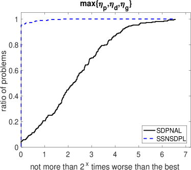
(a) opt

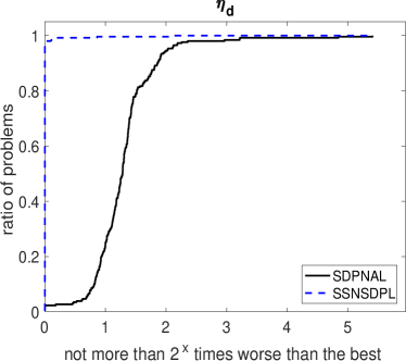
(b) $\eta_{d}$

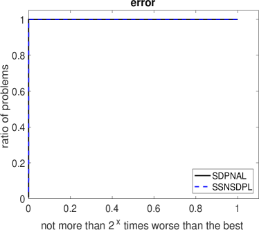
(c) error

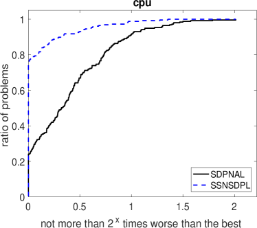
(d) CPU

Fig. 4: The performance profiles of SDPNAL and SSNSDPL

6 Conclusion

In this paper, we consider the v2-RDM model for approximating the solution to the molecular Schrödinger equation. Instead of computing the smallest eigenvalue of the many-electron Schrödinger operator, we minimize the total energy of the many-electron system with respect to 1-RDM and 2-RDM subject to some linear constraints imposed to enhance the $N$-representability of the decision variables. The minimization problem to be solved is an SDP. The solution of the SDP can be obtained from the solution of a system of nonlinear equations that can be derived from a fixed point iteration of DRS applied to the original SDP. We present a semi-smooth Newton type method for solving this set of nonlinear equations. A hyperplane projection technique is applied to improve the stability of the method and achieve global convergence. We exploit the block diagonal structure and low rank structure of the variables in the SDP to improve the computational efficiency. The computational results show that the proposed semi-smooth Newton method can achieve higher accuracy, and is competitive with the Newton-CG Augmented Lagrangian Method for solving SDPs.

Several components of the proposed semi-smooth Newton method can be further improved. For example, since eigenvalue decomposition is the most expensive step in the procedure for computing the Newton direction, a more efficient eigen-decomposition methods needs to be investigated. A better global convergent technique is also needed to improve the overall performance.

References

- [1] H. H. Bauschke and P. L. Combettes, Convex analysis and monotone operator theory in Hilbert spaces, Springer, New York, 2011.
- [2] S. Boyd, N. Parikh, E. Chu, B. Peleato, and J. Eckstein, Distributed optimization and statistical learning via the alternating direction method of multipliers, Foundations and Trends® in Machine Learning, 3 (2011), pp. 1–122.
- [3] B. J. Braams, J. K. Percus, and Z. Zhao, The t1 and t2 representability conditions, Advances in Chemical Physics, Volume 134: Reduced-Density-Matrix Mechanics: With Application to Many-Electron Atoms and Molecules, 165 (2007), p. 93.
- [4] D. Chaykin, C. Jansson, F. Keil, M. Lange, K. T. Ohlhus, and S. M. Rump, Rigorous results in electronic structure calculations, (2016).
- [5] L. Chen, D. Sun, and K.-C. Toh, A note on the convergence of admm for linearly constrained convex optimization problems, Computational Optimization and Applications, 66 (2017), pp. 327–343.
- [6] A. J. Coleman, Structure of fermion density matrices, Rev. Mod. Phys., 35 (1963), p. 668.
- [7] E. D. Dolan and J. J. Moré, Benchmarking optimization software with performance profiles, Mathematical programming, 91 (2002), pp. 201–213.
- [8] J. Douglas and H. H. Rachford, On the numerical solution of heat conduction problems in two and three space variables, Trans. Amer. Math. Soc., 82 (1956), pp. 421–439.
- [9] J. Eckstein and D. P. Bertsekas, On the douglas–rachford splitting method and the proximal point algorithm for maximal monotone operators, Mathematical Programming, 55 (1992), pp. 293–318.
- [10] J. Eckstein and D. P. Bertsekas, On the Douglas-Rachford splitting method and the proximal point algorithm for maximal monotone operators, Math. Program., 55 (1992), pp. 293–318.
- [11] R. Erdahl, Representability, International Journal of Quantum Chemistry, 13 (1978), pp. 697–718.
- [12] D. Gabay and B. Mercier, A dual algorithm for the solution of nonlinear variational problems via finite element approximation, Computers & Mathematics with Applications, 2 (1976), pp. 17–40.
- [13] C. Garrod and J. K. Percus, Reduction of the N-Particle Variational Problem, J. Math. Phys., 5 (1964), p. 1756.
- [14] G. Gidofalvi and D. A. Mazziotti, Spin and symmetry adaptation of the variational two-electron reduced-density-matrix method, Phys. Rev. A - At. Mol. Opt. Phys., 72 (2005), pp. 1–8.
- [15] P.-L. Lions and B. Mercier, Splitting algorithms for the sum of two nonlinear operators, SIAM J. Numer. Anal., 16 (1979), pp. 964–979.
- [16] Y. K. Liu, M. Christandl, and F. Verstraete, Quantum computational complexity of the N-representability problem: QMA complete, Phys. Rev. Lett., 98 (2007), pp. 1–4.
- [17] J. E. Mayer, Electron correlation, Physical Review, 100 (1955), p. 1579.
- [18] D. A. Mazziotti, Variational reduced-density-matrix method using three-particle n-representability conditions with application to many-electron molecules, Physical Review A, 74 (2006), p. 032501.
- [19] D. A. Mazziotti, Large-scale semidefinite programming for many-electron quantum mechanics, Phys. Rev. Lett., 106 (2011), pp. 7–10.
- [20] R. Mifflin, Semismooth and semiconvex functions in constrained optimization, SIAM J. Control Optim., 15 (1977), pp. 959–972.
- [21] M. Nakata, B. J. Braams, K. Fujisawa, M. Fukuda, J. K. Percus, M. Yamashita, and Z. Zhao, Variational calculation of second-order reduced density matrices by strong N -representability conditions and an accurate semidefinite programming solver, J. Chem. Phys., 128 (2008).
- [22] M. Nakata, H. Nakatsuji, M. Ehara, M. Fukuda, K. Nakata, and K. Fujisawa, Variational calculations of fermion second-order reduced density matrices be semidefinite programming algorithm, J. Chem. Phys., 114 (2001), pp. 8282–8292.
- [23] G. Pataki, On the rank of extreme matrices in semidefinite programs and the multiplicity of optimal eigenvalues, Mathematics of operations research, 23 (1998), pp. 339–358.
- [24] L. Q. Qi and J. Sun, A nonsmooth version of Newton’s method, Math. Programming, 58 (1993), pp. 353–367.
- [25] R. T. Rockafellar and R. J.-B. Wets, Variational analysis, Springer-Verlag, Berlin, 1998.
- [26] Y. Saad, J. R. Chelikowsky, and S. M. Shontz, Numerical methods for electronic structure calculations of materials, SIAM Rev., 52 (2010), pp. 3–54.
- [27] D. C. Sherrill and H. F. Schaefer, The configuration interaction method: Advances in highly correlated approaches, Advances in Quantum Chemistry, 34 (1999), pp. 143 – 269.
- [28] M. V. Solodov and B. F. Svaiter, A globally convergent inexact Newton method for systems of monotone equations, in Reformulation: nonsmooth, piecewise smooth, semismooth and smoothing methods (Lausanne, 1997), M. Fukushima and L. Qi, eds., vol. 22, Kluwer Academic Publishers, Dordrecht, 1999, pp. 355–369.
- [29] D. Sun and J. Sun, Semismooth matrix-valued functions, Math. Oper. Res., 27 (2002), pp. 150–169.
- [30] D. Sun, K.-C. Toh, and L. Yang, A convergent 3-block semiproximal alternating direction method of multipliers for conic programming with 4-type constraints, SIAM J. Optim., 25 (2015), pp. 882–915.
- [31] S. Szalay, M. Pfeffer, V. Murg, G. Barcza, F. Verstraete, R. Schneider, and Ö. Legeza, Tensor product methods and entanglement optimization for ab initio quantum chemistry, Int. J. Quantum Chem., 115 (2015), pp. 1342–1391.
- [32] J. Čížek, On the Correlation Problem in Atomic and Molecular Systems. Calculation of Wavefunction Components in Ursell-Type Expansion Using Quantum-Field Theoretical Methods, Journal of Chemical Physics, 45 (1966), pp. 4256–4266.
- [33] Z. Wen, D. Goldfarb, and W. Yin, Alternating direction augmented Lagrangian methods for semidefinite programming, Math. Program. Comput., 2 (2010), pp. 203–230.
- [34] X. Xiao, Y. Li, Z. Wen, and L. Zhang, A regularized semi-smooth newton method with projection steps for composite convex programs, arXiv preprint arXiv:1603.07870, (2016).
- [35] L. Yang, D. Sun, and K. C. Toh, SDPNAL+: a majorized semismooth Newton-CG augmented Lagrangian method for semidefinite programming with nonnegative constraints, Math. Program. Comput., 7 (2015), pp. 331–366.
- [36] X.-y. Zhao, D. Sun, and K. C. Toh, A Newton-CG Augmented Lagrangian Method for Semidefinite Programming ∗, SIAM J. Optim., 117543 (2009), pp. 1–40.
- [37] Z. Zhao, B. J. Braams, M. Fukuda, M. L. Overton, and J. K. Percus, The reduced density matrix method for electronic structure calculations and the role of three-index representability conditions., J. Chem. Phys., 120 (2004), pp. 2095–104.