Gatherplots: Generalized Scatterplots for Nominal Data

Abstract

Overplotting of data points is a common problem when visualizing large datasets in a scatterplot, particularly when mapping nominal dimensions to one of the scatterplot axes. Transparency, aggregation, and jittering have previously been suggested to address this issue, but these solutions all have drawbacks for assessing the data distribution in the plot. We propose gatherplots, an extension of scatterplots that eliminates overplotting, particularly for nominal variables. In gatherplots, every data point that maps to the same position coalesces to form a stacked entity, thereby making it easier to compare the absolute and relative sizes of data groupings. The size and aspect ratio of data points can also be changed dynamically to make it easier to compare the composition of different groups. Furthermore, several embedded interaction techniques support slicing and dicing the gatherplot by pivoting on particular dimensions, ranges, and values in the dataset. Our evaluation shows that gatherplots enable users from the general public to judge the relative portion of subgroups more quickly and more correctly than when using conventional scatterplots with jittering. Furthermore, a review conducted by a group of visualization experts evaluated and commented on the gatherplot design.

Introduction

Scatterplots—one of the most widely used types of statistical graphics [7, 12, 34]—are commonly used to visualize two continuous variables using visual marks mapped to a two-dimensional Cartesian space, where the color, size, and shape of the marks can represent additional dimensions. However, scatterplots are so-called overlapping visualizations [15] in that the visual marks representing individual data points may begin to overlap each other in screen space in situations when the marks are large, when there is insufficient screen space to fit all the data at the desired resolution, or simply when several data points share the same value. The latter is particularly problematic for discrete variables with small domains, such as for nominal and ordinal data [31], due to the increased incidence of shared values. This kind of overlap is known as overplotting (or overdrawing) in visualization, and is problematic because it may lead to data points being entirely hidden by other points, which in turn may lead to the viewer making incorrect assessments of the data. In particular, the issue with small-domain discrete variables has led to scatterplots being almost exclusively used for continuous variables; Figure Gatherplots: Generalized Scatterplots for Nominal Data(a) shows an example of what happens if a data dimension mapped to an axis has this discrete property.

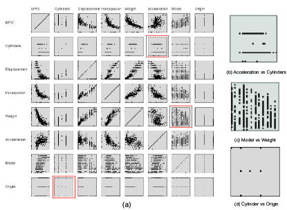
Figure 1: Limitations of scatterplots for managing discrete variables. (a) The scatterplot matrix for 7-dimensional car dataset. (b) The acceleration vs. cylinders scatterplot looks like a horizontal line because the ordinal cylinders axis has been mapped onto the graphical Y axis. (c) The model vs. weight scatterplot shows vertical lines due to the model year behaving as a discrete ordinal value, which causes overplotting. (d) The cylinders vs. origin scatterplot shows dotted patterns because discrete dimensions have been mapped onto both the X and Y axis.

However, realistic multidimensional datasets often contain a combination of both continuous and discrete data dimensions, and even if a dataset is entirely continuous, the physical limitations of computer screens means that overplotting may (and most likely will) still occur even if no value overlap exists in the data (Figure 1). Several approaches have been proposed to address this problem [11], the most prominent being transparency, clustering, and jittering. The first of these, transparency, does not so much address the problem as sidestep it by making the visual marks semi-transparent so that an accumulation of overlapping points in the same are still visible. However, this will not scale well for large datasets, and also causes blending issues if color is used to encode additional variables. Clustering, on the other hand, attempts to organize overlapping marks into visual groups that summarize the distribution [16, 23], but increases the complexity of the scatterplot. Finally, jittering perturbs visual marks using a random displacement [32] so that no mark falls on the exact same screen location as any other mark (Figure Gatherplots: Generalized Scatterplots for Nominal Data(b)), but this approach is still prone to overplotting for large datasets. Jittering also introduces uncertainty in the data that is not aptly communicated by the scatterplot since marks will no longer be placed at their true location on the Cartesian space.

In this paper, we propose the concept of gathering as an alternative to scattering and jittering, and then show how we can use this visual transformation to define a novel visualization technique called a gatherplot. Gathering is a generalization of the linear mapping used by scatterplots, and works by partitioning the graphical axis into segments based on the data dimension and then organizing points into stacked groups for each segment that avoids overplotting. This means that the gather operation relaxes the continuous spatial mapping traditionally used for a graphical axis; instead, each discrete segment occupies a certain amount of screen space that is all defined to map to the exact same data value. This is communicated using graphical brackets on the axis that shows the value or interval for each segment (Figure Gatherplots: Generalized Scatterplots for Nominal Data(c)).

The gatherplot technique, then, is merely a scatterplot where the gather transformation is used on one or both of the graphical axes. Additional data dimensions can be used to cluster together different points within a stacked group; Figure Gatherplots: Generalized Scatterplots for Nominal Data shows how the origin of cars, communicated using color, is also used to organize these marks into discrete groupings. Furthermore, if the user is trying to assess relative proportions rather than absolute numbers, the aspect ratio of the visual marks in each stacked group can be changed independently to fill the available space (Figure Gatherplots: Generalized Scatterplots for Nominal Data(d)). Because we define a common model for scatterplots, jitterplots, and gatherplots alike, our prototype implementation makes it easy to transition freely between them.

The contributions of our paper are the following: (1) the concept of the gather visual transformation as a generalization of linear visual mappings; (2) the gatherplot technique, an application of the gather operation to scatterplots to solve the overplotting problem; and (3) results from both a crowdsourced graphical perception evaluation studying effectiveness of gatherplots compared to jitterplots as well as an expert review involving multiple visualization experts using the technique for in-depth data analysis. In the remainder of this paper, we first review the literature on statistical graphics and overplotting. We then present the gather operation and use it to define gatherplots. This is followed by our crowdsourced evaluation and expert review. We close with implementation notes, conclusions, and our future plans.

1 Background

Our goal with gatherplots is to generalize scatterplots to a representation that maintains its simplicity and familiarity while eliminating overplotting. With this in mind, below we review prior art that generalizes scatterplots for mitigating overplotting. We also discuss related visualization techniques specifically designed for nominal variables.

1.1 Characterizing Overplotting

While there are many ways to categorize visualization techniques, a particularly useful classification for our purposes is one introduced by Fekete and Plaisant [15], which splits visualization into two types:

• Overlapping visualizations: These techniques enforce no layout restrictions on visual marks, which may lead to them overlapping on the display and causing occlusion. Examples include scatterplots, node-link diagrams, and parallel coordinates.

• Space-filling visualizations: A visualization that restricts layout to fill the available space and to avoid overlap. Examples include treemaps, adjacency matrices, and choropleth maps.

Fekete and Plaisant [15] investigated the overplotting phenomenon for a 2D scatterplot, and found that it has a significant impact as datasets grow. The problem stems from the fact even with two continuous variables that do not share any coordinate pairs, the size ratio between the visual marks and the display remains more or less constant. Furthermore, most datasets are not uniformly distributed. This all means that overplotting is bound to happen for realistic datasets.

Ellis and Dix [11] survey the literature and derive a general approach to reduce clutter. According to their treatment, there are three ways to reduce clutter in a visualization: by changing the visual appearance, through space distortion, or by presenting the data over time. Some trivial but impractical mechanisms they list include decreasing mark size, increasing display space, or animating the data. Below we review more practical approaches based on appearance and distortion.

1.2 Appearance-based Methods

Practical appearance-based approaches to mitigate overplotting include transparency, sampling, kernel density estimation (KDE), and aggregation. Transparency changes the opacity of the visual marks, and has been shown to convey overlap for up to five occurrences [36]. However, there is still an upper limit for how much overlap is perceptible to the user, and the blending caused by overlapping marks of different colors makes identifying specific colors difficult. Sampling uses stochastic methods to statistically reduce the data size for visualization [10]. This may reduce the amount of overplotting, but since the sampling must be random, it can never reliably eliminate it.

KDE [30] and other binned aggregation methods [13, 16] replace a cluster of marks with a single entity that has a distinct visual representation. However, these methods are difficult to apply for scatterplots because scatterplots operate on the principle of object identity, meaning that each visual mark is supposed to represent a single entity. Splatterplots [23] overcome this by overlaying individual marks side-by-side with the aggregated entities, using marks to show outliers and aggregated entities to show the general trends. However, even with only few aggregated entities, the resulting color-blended image becomes visually complex and challenging to read and understand.

1.3 Distortion-based Methods

Unfortunately, appearance-based clutter reduction methods [11] are not well-suited for discrete variables, since such dimensions may cause many data points to map to the exact same screen location. In such a situation, changing the appearance of the marks does not help. For such data, distortion-based techniques may be better. The canonical distortion technique is jittering, where a random displacement is used to subtly modify the exact screen space position of a data point. This has the effect of spreading data points apart so that they are easier to distinguish. However, most naïve jittering mechanisms apply the displacement indiscriminately to all data points, regardless of whether they are overlapping or not. This has the drawback of distorting all points away from their true location on the visual canvas, and still does not completely eliminate overplotting.

Bezerianos et al. [3] use a more structured approach to displacement, where overlapping marks are organized onto the perimeter of a circle. The circle is grown to a radius where all marks fit, which means that its size is also an indication of the number of participating points. However, this mechanism still introduces uncertainty in the spatial mapping, and it is also not clear how well it scales for very dense data. Nevertheless, it is a good example of how deterministic displacement can be used to great effect for eliminating overplotting.

Trutschl et al. [32] propose a deterministic displacement (“smart jittering”) that adds meaning to the location of jittering based on clustering results. Similarly, Shneiderman et al. [29] propose a related structured displacement approach called hieraxes, which combines hierarchical browsing with two-dimensional scatterplots. In hieraxes, a two-dimensional visual space is subdivided into rectangular segments for different categories in the data, and points are then coalesced into stacked groups inside the different segments. This idea is obviously very similar to our gatherplots technique, but the main difference is that we in this paper derive gatherplots as generalizations of scatterplots, and also define mechanisms for laying out the stacked groups, organizing them by another dimension, and modifying their aspect ratio to support relative assessments.

1.4 Visualizing Nominal Variables

While we have already ascertained that scatterplots are not optimal for nominal variables, there exists a multitude of visualization techniques that are [1, 20, 22]. Simplest among them are histograms, which allows for visualizing the item count for each nominal value [31], but much more complex representation are possible. One particular usage for visualizing nominal data that is of practical interest is for making inferences based on statistical and probabilistic data. Cosmides and Toody [9] used frequency grids as discrete countable objects, and Micallef et al. [25] build extend this with six different area-proportional representations of nominal data organized into different classes.

As a parallel to our work on gatherplots, one particular multidimensional visualization technique that is closely related to scatterplots is parallel coordinate plots [21]. However, just like scatterplots, parallel coordinate plots are often plagued by overplotting due to high data density and discrete data dimensions. The work by Kosara et al. [22] to extend parallel coordinate plots into parallel sets is interesting because it specifically addresses the overplotting concern by grouping points with the same value into a segment on the parallel axis. This is precisely the same idea we will apply for scatterplots in this work.

2 The Gather Transformation

Position along a common scale is the most salient of all visual variables [2, 8], and so mapping a data dimension to positions on a graphical axis is a standard operation in data visualization. We call this mapping a visual transformation. However, most statistical treatments of data, such as Stevens’ classical theory on the scale of measurements [31], do not take the physical properties of display space into account. This is our purpose in the following section.

2.1 Problem Definition

Let $V=<f,s>$ be a visual transformation that consists of a transformation function $f$ and a mark size $s$. Furthermore, assume that $f$ transforms a data point $p_{d}\in D$ from a data dimension $D$ to a coordinate on a graphical axis $p_{c}\in C$ by $f(p_{d})=p_{c}$. Given a dataset $D_{i}\subseteq D$, we say that a particular visual transformation $V_{j}$ exhibits overlap if

$$\exists p_{x},p_{y}\in D_{i}\wedge x\neq y:|f_{j}(p_{x})-f_{j}(p_{y})|<s_{j}.$$

In other words, overlap occurs for a particular dataset and visual transformation if there exists at least one case where the visual marks of two separate data points in the dataset fall within the same interval on the graphical axis. The overlap index of a dataset and visual transformation is defined as the number of unique pairs of points that overlap. For a one-dimensional visualization, only a single transformation is used and the visualization and dataset is said to exhibit overplotting iff it exhibits overlap. For a two-dimensional visualization, however, the visualization and dataset will only exhibit overplotting iff there is overlap in both visual transformations and data dimensions. Analogously, the overplotting index is the unique number of overplotting incidences for that particular visual transformation and dataset.

This has two practical implications: (1) even a dataset that consists only of nominal variables may not exhibit overplotting if there is only at most one instance of each nominal value, and (2) a dataset consisting of continuous values may still exhibit overplotting if any two points in the dataset are close enough that they get mapped to within the size of the visual marks on the screen. The corollary is basically that overplotting is a function of both visualization technique and dataset.

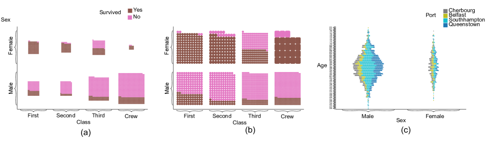
Figure 2: Main layout modes for gatherplots: (a) absolute mode with constant aspect ratio, which arranges items following the aspect ratio of given area; (b) relative mode of (a). The rate of survivors in each male passenger class is not each to compare. Figure (c) shows the streamgraph mode, where each cluster maintains the number of element in the shorter edge, making it easier to see the distribution of the subgroups along the Y axis.

2.2 Definition: The Gather Transformation

We build on the previous idea of structured displacement [3, 29] by proposing a novel visual transformation function called a gather transformation $f_{gather}$ that non-linearly segments the graphical axis $C$ and organizes data points in each segment to eliminate overplotting.

The gather transformation $V_{gather}=<f_{gather},s_{gather}>$ consists of a transformation function $f_{gather}$ that maps data points $p_{d}\in D$ to coordinates $p_{c}\in C$, and a visual mark sizing function (instead of a scalar) $s_{gather}$ that yields a visual mark size given the same data point. The gather transformation function is special in that it eliminates overplotting by subdividing the graphical axis $C$ into $n$ contiguous segments $C=\{C_{1},C_{2},\ldots,C_{n}\}$, where $n$ is the size of the domain of the gather transformation function, i.e., the number of unique elements in the data dimension $D$. When mapping a data point $p_{d}$ to the graphical axis, $f_{gather}$ will return an arbitrary graphical coordinate $p_{c}\in C_{i}$ for whatever coordinate segment $C_{i}$ that $p_{d}$ belongs to.

Practically speaking, coordinates $p_{c}\in C_{i}$ will be chosen to efficiently pack visual marks into the available display space without causing overplotting (i.e., using a regular spacing of size $s_{gather}$). Several different methods exist for adapting the gather transformation to the dataset $D$. One approach is to keep the segments $C_{1},\ldots,C_{n}$ of equal size and find a constant visual mark size $s_{gather}(p_{d})=s_{max}$ that ensures that all points fit within the most dense segment. The constant mark size makes visual comparison straightforward. Another approach is to adapt segment size to the density of the data while still keeping the mark size constant. This will minimize empty space in the visual transformation and allows for maximizing mark size. A third approach is to vary mark size proportionally to the number of points in a segment. This will make comparison of the absolute number of points in each segment difficult, but may facilitate relative comparisons if marks are distinguished in some other way (e.g., using color).

For data dimensions $D$ that have a very large number of unique values, it often makes sense to first quantize the data using a function $p_{q}=Q(p_{d})$ so that the number of elements $n$ is kept manageable (on the order of 10 or less for most visualizations). For example, a data dimension representing a person’s age might heuristically be quantized into ranges of 10 years: 0-9 years, 10-19 years, 20-29 years, and so on.

In a gather transformation, the coordinate axis has been partitioned into segments, where the order of segments on the axis depends on the data. For nominal data, the segments can be reordered freely, both by the algorithm and by the user. For ordinal or quantized data, the order is given by the data relation. Furthermore, it often makes sense to be able to order points inside each segment $C_{i}$ using the gathering transformation function $f_{gather}$, for example using a second data dimension (possibly visualized using color) to group related items together.

Appropriate visual representations of data where the gather transformation has been applied are also important. The stacked entities of gathered points—one per coordinate segment $C_{i}$—should typically maintain object identity, so that each constituent point and their size is discernible as a discrete visual mark. Similarly, a visual representation of the segmented graphical axis should externalize the segments as labeled intervals instead of labeled major and minor ticks; this will also communicate the discontinuous nature of the axis itself to the viewer.

2.3 Using the Gather Transformation

To give an example in one-dimensional space, parallel coordinate plots [21] use multiple graphical axes, one per dimension $D_{i}$, and organize them in parallel while rendering data points as polylines connecting data values on one axis to adjacent ones. However, traditional parallel coordinate plots merely use a scatter transformation on each graphical axis, which makes the technique prone to overplotting. Multiple authors have studied ways of mitigating this problem, for example by reorganizing the position of nominal values [28], using transparency, applying jitter, or by clustering the data [16].

However, an alternative approach is to use the gather representation for each graphical axis to minimize overplotting. This will cause each axis to be segmented into intervals, and we can then resize segments according to the number of items falling into each segment so that segments with many data points become proportionally larger than those with fewer points. Finally, if the data dimensions represent nominal data, it may make sense to use a global segment ordering function so that there is a minimum of lateral movement for the majority of points as they connect to adjacent axes. This will also minimize line crossings between the parallel axes. This particular visualization technique—a parallel coordinate plot with the gather transformation applied to each graphical axis—is essentially equivalent to parallel sets [22].

In fact, by applying our generalized gather transformation to the axis, we are actually proposing a new type of stacked visualization where each entity is still represented by lines. In a sense, this technique combines parallel coordinates and parallel sets because the grouped lines maintain the illusion of a single entity for an axis with nominal categorical values (similar to parallel sets), yet integrates directly with a parallel coordinate axis with continuous values. The main difference is that the new parallel coordinate/set variation allows each axis to be either categorical or continuous, meaning that one axis can represent the gender and the next can represent the height of person.

3 Gatherplots: A 2D Gathering Representation

Here we apply the concept of gathering to the scatterplots to alleviate overplotting, focusing on optimal layouts of gathered entities, graphical representations of chart elements, and novel interactions.

3.1 Applying Gathering to Perpendicular Axes

The application of the gather transformation results in the segmentation of output range of an axis scale, where the items with same values will be arranged to avoid overplotting. Applying gathering to two perpendicular axes defining a Cartesian space results in a gatherplot: a 2D visualization technique that aggregates entities for each axis. However, given this basic visual representation, there are many open design possibilities for aspect ratio, layout, and item shapes. We discuss these design parameters in the treatment below.

3.2 Layout Modes

Gatherplots organizes entities into stacked groups according to a discrete variable to eliminate overplotting. However, the result depends on the context, especially on the size distribution of each groups, the aspect ratio of assigned space, and the task at hand. This makes finding an optimal layout difficult. One solution is to provide interaction techniques to change the layout, but such layout options may lead to confusion for the user. Our approach is to provide one general optimal visualization for the most common aspect ratio and tasks, and provide a very few optional methods to change it. As a result, we derive the following three layout modes (examples in Figure 2):

• Absolute mode. Here stacked groups are sized to follow the aspect-ratio of the assigned region. The node size of the items are determined by the maximum length dots which can fill the assigned region without overlapping. This means with the same assigned space, the groups with the maximum number of members determines the overall size of the nodes.

• Relative mode. In this mode, the node size and aspect ratio is adapted so that every stacked group has equal dimensions. This is a special mode to make it easier to investigate ratios when the user is interested in the relative distributions of subgroups rather than the absolute number of members. Items also change their shape from a circle (absolute mode) to a rectangle.

• Streamgraph mode. Here stacked groups are reorganized so that the maintain the same number of elements in their shorter edge. This mode is used for regions where the ratio of width and height are drastically different (in our prototype implementation, we use a heuristic value of 3 for aspect ratio to be a threshold for activating this mode). This means there are usually many times more groups in the axis in parallel with shorter edges. The purpose of this mode is to make it easier to compare the size along these many entities. The resulting graphic resembles ThemeRiver [18] as the number of entities increase.

The choice between absolute mode and streamgraph mode happens automatically based on the aspect ratio and without user intervention. Therefore only interactive option is required to toggle between absolute mode and relative mode. Our intuition is that the absolute mode should be good enough for most of the time, and when very specific tasks are required, the user can switch to the relative modes.

However, gatherplots involve many more possibilities beyond than these layout functions. Below follows our treatment of these design possibilities and our rationale for our decisions.

3.2.1 Area vs. Length Oriented Layout

Maintaining the aspect ratio of all stacked groups means that the size of the group is represented by its area. The length of the group is only used in special cases when the aspect ratio is very high or low. According to Cleveland and McGill [8], length is far more effective than the area for graphical perception. However, Figure 3 shows the three problems associated with layout to enable length-based size comparison. In this view, the items are stacked along the vertical axis to make the size comparison along the horizontal axis easier. The width of rectangle is all set to be equal to so that the length can represent the size of subgroups. However, they show drastically different shape of line vs. rectangle, which may cause users to lose concept of equality. Furthermore, to make length-based comparison easier, the stacking should be aligned to one side of the available space: left, right, top, or bottom.

In this case, the bottom is selected to make it easier to compare along the X axis. However, this creates additional two problem. The first problem is that center of mass of each stacked group is so different that the concept of belonging to the same value can be misleading. The second problem is that choosing alignment direction is arbitrary and depends on the task. For example, in this view it is more difficult to compare along the Y axis. In this sense, this layout is biased to the X axis, while sacrificing the performance along the Y axis. For this reason, the most general choice is to use center alignment with aspect ratio resembling the assigned range to avoid bias.

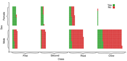
Figure 3: Stacked group layouts for gathering. This layout supports comparison group sizes. Because the height of stacked groups is all fixed to the same value, comparing the length yields the size.

3.2.2 Uniform vs. Variable Area Allocation

In gatherplots, we assign uniform range to different values of overlappable variables. For some cases, assigning variable area can make sense and create interesting visualizations. As a simple example, we can argue that assigning the range of output for gather transfer function to be proportional to the numbers of items that belong that value uses the space most efficiently. This will result in the following layout shown in Figure 4, which is basically a mosaic plot [17].

Figure 4: Variable area for a gatherplot. The chart uses space efficiently. Items which belong to same place should belong to the same value. However, as can be shown in the Y axis tick marker, this results in a violation of the scatterplot concept.

3.2.3 Role of Relative Mode

Since gathering assigns a discrete noncontinuous range to each graphical axis, each stacked group can be grown to fill all available space. This relative mode is useful for two specific tasks:

• Getting a relative percentage of the subgroups in the group (Figure 2). Because groups of different size is normalized to the same size, any comparison in area results in a relative comparison.

• Finding the distribution of outliers. When there are many items on the screen for absolute mode, all node sizes must be reduced. This can make outliers hard to locate.

3.3 Graphical Representations

In this section, we discuss the visual representation for gatherplots and how it differs from traditional scatterplots.

3.3.1 Continuous Color Dimension

The gather transform sorts items according to a data property, such as a variable also assigned for coloring items. This removes the scattered color patterns in the stacked groups that is common in other techniques such as Gridl [29]. This is also particularly useful for continuous color scales, making the variation of colors are easier to perceive (Figure 5).

Figure 5: Continuous color scale used in a gatherplot. The X axis is origins of cars and the Y axis is MPG. The color scale is acceleration.

3.3.2 Shape for Items

Scatterplots typically use a small circle or dot as a visual representation for items, but many variations exist that use glyph shapes to convey multidimensional variables[24, 33, 4, 7, 5]. However, in the relative mode, sometimes the aspect ratio of nodes changes according to the aspect ratio of box assigned to that value. Also, as gathering changes the size of nodes to fit in one cluster, sometimes node size becomes too small, or too large compared to other nodes. This results in several unique design considerations for item shapes. After trying various design alternatives, we recommend using a rectangle with constant rounded edge without using stroke lines. Using constant rounded edge allows the nodes to be circular when the node is small, as in Figure 2(b), and a rectangle to show the degree of stretching, as shown in Figure 2(b). Figure 6 shows some previous trials with various shapes.

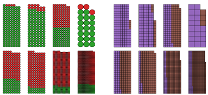
Figure 6: Stroke line problems where the circle consumes ample white space between adjacent nodes, which contributes to clutter as it grows. The rectangle does not have space between nodes, however, it must have a stroke border to show stretching. But this borderline creates problems when the items are very small.

3.3.3 Design of Tick Marks

The single line type tick marks for scatterplots are not appropriate for gatherplots. Because we are representing a range rather than a single point, a range tick marker will be better. Without this visual representation, when the user is confronted with a number, it can be confusing to determine whether adjacent nodes with different offset has same value or not. After considering a few visual representation, we recommend a bracket type marker for this purpose. Figure 7 shows various types of markers for range representation. The bracket is optimal in that it uses less ink and creates less density with adjacent ticks.

Figure 7: Various tick marks types. The blue dotted region represents the area between adjacent tick marks. (a) is a typical line type tick mark for the scatterplots. (b) lacks guide lines, which will make anchoring easier. (c) creates a packed region between adjacent marks. (d) uses less crowded region in this regionn, but (e) is the least crowded. (f) is the final recommendation, with the data label in the orange region.

3.3.4 Tick Labels for Numbers

In gatherplots, a tick mark represents a range. This creates a problem for the data label. Because it is a number, the naïve way to represent will be having beginning number and ending number at each side, as shown in Figure 8. However this creates a very dense region between adjacent marks and, worse, the same number is repeated in this region, thereby wasting space. We recommend the use of a plus-minus sign to represent a bin size, to create a conceptually consistent tick labels. One limitation with this approach is the binning of arbitrary size can create bins of arbitrary floating number occupying an inappropriate amount of size.

Figure 8: Several different tick label designs, including (a) numbers (used for nominal values), (b) extents of a range, and (c) the size of the range.

3.3.5 Extension of Scatterplot Matrix

One subtle difficulties in working with scatterplot matrix is when the users want to see only single axis, without definition in other axis. Or one may assigning same dimension to the X and Y axes while exploring various dimensions. Both will create an overdrawing in a traditional scatterplot matrix. However, in gatherplots, an undefined axis result in the aggregation of all nodes in one group, which is a spontaneous logical extension. This enables the scatterplots matrix to have an additional row and column with undefined axes. Figure 9 shows an example of this using cars dataset. Two dimensions—displacement and MPG—were used to create a 3 by 3 gatherplots matrix. Note that 7 out of 9 charts are new compared to scatterplots, while adding information to the whole picture. The diagonals also enable seeing distribution, which is a improvement over previous scatterplots matrix.

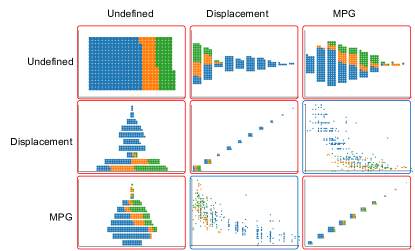
Figure 9: This shows the power of an undefined axis using an example of a gatherplots matrix for the cars dataset. Two continuous variables, Displacement and MPG, are used. The charts in the red box are new addition to the previous scatterplots matrix, while the charts in the blue box remains the same. Using the undefined axis enabled creating an informative chart showing the distribution of only single variable with a streamgraph type graphic. The upper right corner of the matrix shows undefined vs. undefined, which is logically representing all the items.

3.3.6 Applications for Continuous Variables

Gatherplots can be used to mitigate overplotting caused by continuous variables as well. Figure 10 (a) shows how gatherplots handle the overplotting caused by continuous variables. The plot is using relative mode with two random variables. The relative mode makes it easier to identify the outliers and the distribution of outliers.

One limitation of gatherplots is that it requires binning to manage a continuous variable, yet binning creates arbitrary boundaries. In this sense, gatherplots can be misleading. However, combining gatherplots with scatterplots makes this problem less severe.

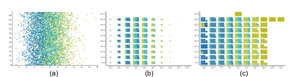
Figure 10: Using gatherplots to manage overplotting. (a) shows a scatterplot with 5,000 random numbers with severe overplotting in the center area. In (b), gathering is applied to create a more organized view. However, the gathering resizes the items so small that it becomes difficult to detect outliers. (c) shows relative mode, where the outliers are enlarged. This makes identifying the distribution of sparse regions easier.

3.3.7 Animated Transitions

The many shape and layout transitions involved in gatherplots can be confusing to users. Animation can be a powerful tool to reduce this and maintain the user’s mental model. Heer and Robertson investigated the effectiveness of animated transitions and found that animating the statistical chart can improve the perception of statistical data[19]. Robertson et al. [27] found that animation leads to an enjoyable and exciting experience, even ifx the analysis was not effective. Elmqvist et al. [12] used animation for the scatterplots to maintain congruence. Drawing on all of this work, gatherplots uses animated transitions for all state and layout changes. In addition to the animation according to the axis dimension change, animation is used to show thx transition between scatterplots and jitterplots. This ameliorates the potential misconception of the data distribution in the gatherplots.

3.3.8 Axis Folding Interaction

As an exploration tool for real-world dataset, it is crucial to have means to filter unwanted data. To aid this process with gather transform, we provide an optional mechanism to go back to the original continuous linear scale function. We allow each axis tick have an interactive control to be filtered out (minimize) or focused (maximized). This is called axis folding, because it can be explained mentally by a folding paper. When minimized or folded, the visualization space is shrunk by applying linear scales instead of nonlinear gather scales. This results in overplotting as if a scatterplot was used for that axis. A maximization is simply folding all other values except the value of the interest in order to assign maximum visual space to that value. Figure 11 shows the axis folding applied to third class adult passengers in the Titanic dataset.

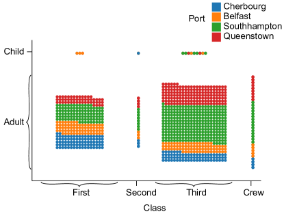
Figure 11: Survivors of the Titanic using a gatherplot. The X axis is class of passengers, where second class passengers and crew are minimized. The Y axis is age, where the adult value is maximized. This view makes it easy to compare first class adults and third class adults. Note that even in the minimized state, we can get an overview about the second class and crew by the color line, which communicates the underlying distribution. This is due to the sorting over the color dimension.

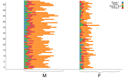
Figure 12: Hypothetical dataset with gender and age. Left alignment makes the distribution along the vertical direction more feasible. Note that only the vales in most left are anchored, so dimensional reordering is required.

4 Implementation

We have implemented a web-based demonstration of gatherplots and published it online. The users can load various dataset and compare each visualization with scatterplots and jittered scatterplots with one button click. In the top right area, an interactive guided walk-through is provided. The users can follow instructions step-by-step to experience gatherplots. In the bottom, a discussion board is provided. The purpose of the discussion board is to accumulate discussions during the expert review. Other people can also join the evaluation process.

The gatherplot prototype implementation was developed using D3.js and Angular.js. Figure  13 shows the screenshot of the implemented website. To test various layout and shape of the nodes, an intermediate version which allows various tweak is also available.

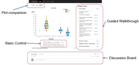
Figure 13: Web-based prototype implementation of gatherplots. Important features are comparison of gatherplots with scatterplots and jittered scatterplots, a guided walkthrough, and a discussion board.

5 Evaluation of Gatherplots using Crowdsourcing

The purpose of this study is to examine the effectiveness of gatherplots especially to see how different modes of gatherplots influence certain types of tasks for the crowdsourced workers. Crowdsourcing platforms have been widely used and have shown to be reliable platforms for evaluation studies [26, 35]. Therefore, we conducted our experiment on Amazon Mechanical Turk  .

5.1 Experiment Design

Gatherplots was developed to overcome limitations of conventional scatterplots. We believe that gatherplots solves the issue of overdrawing, while maintaining structural identity with scatterplots. Jittered scatterplots were selected as a comparison, as it is widely accepted standard technique maintaining same consistency with scatterplots. We also wanted to measure how different modes of gatherplots were effective. Therefore we designed the experiment to have four conditions such as scatterplots with jittering (jitter), gatherplots with absolute mode (absolute), gatherplots with relative mode (relative), and gatherplots with one check button to switch between absolute and relative mode (both). We adopted between-subject design to eliminate learning effect by experiencing other modes. The exact test environment is available for review . Note the questions for each conditions were generated randomly.

5.2 Participants

A total of 240 participants (103 female) completed our survey. Because some questions asked a concept of absolute numbers and probability, we limited demographic to be United States to remove the influence of language. Also to ensure the quality of the workers, qualification of workers were the approval rate of more than 0.95 with number of hits approved to be more than 1,000. Only three of 240 participants did not use English as their first language. 119 people had more than bachelor’s degree, with 42 people having hight school degree. We filtered random clickers, if the time to complete one of questions was shorter than a reasonable time, 5 seconds. Eventually, we have a total of 211 participants.

5.3 Task

Different layouts of gatherplots could support different types of tasks. After reviewing task for nominal variables, we selected three types of task such as retrieving value as a low-level task; comparing and ranking as a high-level task. For the comparing and ranking task, two different types of questions were asked: the tasks to consider absolute values such as frequency and tasks that consider relative values such as percentage. Therefore, for one visualization 5 different questions were generated. For gatherplots, our interest is more about the difference between questions considering absolute values and relative values. The five types of questions are as follows:

• Type 1: retrieve value considering one subgroup

• Type 2: comparing of absolute size of subgroup between groups

• Type 3: ranking of absolute size of subgroup between groups

• Type 4: comparing relative size of subgroup between groups

• Type 5: ranking relative size of subgroup between groups

To reduce the chance of one chart being optimal by luck for specific task, two charts of same problem structure were provided. Eventually, the resulting questions were 10 for each participant. Each question was followed by the question asking confidence of estimation with a 7-point Likert scale, and the time spent for each question was measured.

5.4 Hypotheses

We believe that different types of tasks will favor from different type of layouts. Therefore our hypotheses are as follows:

• For retrieving value considering one subgroup (Type 1), absolute, relative, both mode reduces the occurrence of the error than jitter mode.

• For tasks considering absolute values (Type 2 and 3), the absolute mode reduces the error.

• For tasks considering relative values (Type 4 and 5), the relative mode reduces the error.

5.5 Results

The results were analyzed with respect to the accuracy (correct or incorrect), time spent, and confidence of estimation. Based on our hypotheses, we analyzed the different modes for each type of question: retrieve value, absolute value task, and relative value task.

5.5.1 Accuracy

The number and percentage of participants who answered correct and incorrect answers are shown in Figure 14. Eventually, we had 42 participants for jitter, 56 participants for absolute, 56 participants for relative, and 57 participants fro both mode.

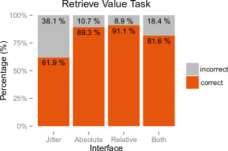
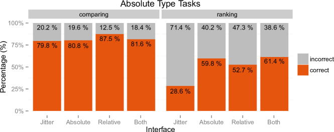
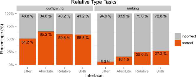
Figure 14: (a) The percentage of participants who have got the answer correct for retrieving value task. (b) The percentage of participants who have got the answer correct for absolute type tasks for comparing and ranking. (c) The percentage of participants who have got the answer correct for relative type tasks for comparing and ranking.

As the measure for each question was either correct or incorrect, a logistic regression was employed using PROC LOGISTICS in SAS. For the retrieving-value task (Type 1), both the the absolute view and relative view had significant main effects (Wald Chi-Square = $18.58$, $p<0.01$, Wald Chi-Square = 21.05, $p<0.01$, respectively) with a significant interaction effect (Wald Chi-Square = 19.53, $p=0.03$) (H1 confirmed). For absolute-value tasks (Type 2 and 3), both the the absolute view and relative view had significant main effects (Wald Chi-Square = 10.35, $p<0.01$, Wald Chi-Square = 10.35, $p<0.01$, respectively) with a significant interaction effect (Wald Chi-Square = 4.31, $p=0.03$) (H2 confirmed). For relative-value tasks (Type 4 and 5), only the relative view had a significant effect (Wald Chi-Square= 5.10, $p=0.02$ ) (H3 confirmed).

5.5.2 Time spent

The time spent (in seconds) for each question was compared using mixed-model ANOVA with repeated measures. For the retrieving-value task, on average, the time spent (sec) for each interface was for jitter (44.26), absolute (56.84), relative (52.45), and both (56.57). There was no significant difference between interfaces ($p>0.05$ for all cases).

For the absolute-value task (Type 2 and 3), on average, the time spent (sec) for each interface was for jitter (30.74), absolute (32.3), relative (33.6), and both (47.91). The interface had a significant main effect ($F(3,207)=11.5,p<0.01$). However, when we conducted pairwise comparisons with adjusted p values using simulation, the only significant difference in time spent was when using the both interface which took longer ($p<0.01$ for all comparisons).

For relative-value task (Type 4 and 5), on average, the time spent for each interface was for jitter (26.6), absolute (31.12), relative (31.38), and both (46.78). The interface had a significant main effect ($F(3,207)=10.12,p<0.01$). However, when we conducted pairwise comparisons with adjusted p values using simulation, the only significant difference in time spent was when using the both interface which took longer ($p<0.01$ for all comparisons).

5.5.3 Confidence

The 7-point Likert-scale rating was used for the level of confidence on their estimation. For the value-retrieving task (Type 1), Kruskal-Wallis non-parametric test revealed that the type of interface had significant impact on the confidence level ($\chi^{2}(3)=74.57p<0.01$). The mean rating for each interface was for jitter (4.8), absolute (6.3), relative (6.0), and both (6.25). A post-hoc Pairwise Wilcoxon Rank Sum test was employed with Bonferroni correction to adjust errors. The jitter interface was significantly lower than the other three modes ($p<0.01$ for all cases). There was no difference between absolute, relative, and both interfaces.

For absolute-value tasks (Type 2 and 3), Kruskal-Wallis non-parametric test revealed that the type of interface had significant impact on the confidence level ($\chi^{2}(3)=18.32,p<0.01$). The mean rating for each interface was jitter (5.4), absolute (5.7), relative (5.0), and both (5.8). A post-hoc Pairwise Wilcoxon Rank Sum test was employed with Bonferroni correction to adjust errors. The interface with both mode was significantly higher than relative and jitter mode ($p<0.01$ for both), however no difference with the absolute mode. The interface with absolute mode was significantly higher than relative and jitter mode ($p<0.01$).

For relative-value tasks (Type 4 and 5), Kruskal-Wallis non-parametric test revealed that the type of interface did not have significant impact on the relative tasks ($\chi^{2}(3)=4.1,p=0.2$). The mean rating was jitter (4.7), absolute (4.9), relative (4.9), and both (4.8).

One possibilities for result is that relative task might be harder than others. The low correct percentage of questions are also shown in Figure 14. To see that, we have tested the confidence level among task types. Kruskal-Wallis non-parametric test revealed that the type of task had significant impact on the confidence level ($\chi^{2}(2)=148.1,p<0.01$). The mean rating for retrieving value (5.9), absolute (5.5), and relative (4.8). The post-hoc Pairwise Wilcoxon Rank Sum test was employed with Bonferroni correction to adjust errors showed that all three task types have significantly different ($p<0.01$ for all cases).

6 Discussions with Experts Feedback

While the performance of executing low level unit task can explain functional part of new visualization, there are more qualitative aspects, such as aesthetics or playfulness. Also the complex interaction techniques and features make it practically difficult to design test with statistical validation. For this reason, complimentary evaluation of visualization technique with experts can be used [14]. To facilitate structured evaluations, a set of tasks and questions were given. The experts were asked to follow the task and write their feedbacks in the discussion board. They could see other people’s comments. After each sessions, we organized feedbacks by moving to an existing thread or creating new topics.

In addition to this, authors requested the on-line data visualization and visual analytics community for opinions. The intention is getting an initial response for adoption. For they are voluntary and free from conflicts of interests, their response can be valuable for general adoption of a new visualization technique.

Because the feedbacks deal with advanced features and design choices, this session is combined with the discussion of issues triggered by the expert reviews.

6.1 Expert Reviews

We were able to get opinions from two graduate students and one professor whose major field is an information visualization. Two sessions with graduate students were conducted in lab environments, where one of authors was available to answer quick questions or provide feedback if necessary. But in general they were asked to follow the on-line guidelines and use discussion board to leave feedbacks. They took about 70 minutes to finish the reviews. The professor was on his own while reviewing. Their original responses were archived and available in the demonstration website at http://www.gatherplot.org.

The responses were positive in general, especially about the aesthetics and the layouts. However many in-depth issues were discovered. Most frequently pointed problems was the difficulty associated with the task of comparing absolute numbers of subgroups between groups of different size. Especially comparison between a large percent subgroup in small group and a small percent subgroup in a large group is difficult. For example, estimating whether the second class female or third class male passengers survived more or not using figure 2 (a) and (b) is difficult. The fundamental reason why this is difficult in gatherplots are because the areas are less effective than the length for perception [6]. This task is well supported by the layout shown in figure 3 12, which was dropped during the design process. However the experts also provided other plausible suggestions to handle better, such as tool-tips, which shows the number of counts in the group. One interesting solution was using the size of small groups as a mask for the anchor box, which will overlaid over the larger groups, so that the size estimation becomes easier.

One interesting suggestion was changing to bar chart or pie chart. For example, when there are only a few items in groups, due to large size of items, the estimation at relative mode can become inaccurate. During the design process, authors implemented this transform, where the rectangle shapes becomes thinner to become lines. However the support for this mode was dropped later, because this mode loses sense of individual entities.

One reviewers suggested a subtle transition where the bin size changes incrementally by small steps to help maintain the sense of object constancy.

Relative mode was commented to be useful to understand the Bayesian inference problem, while one reviewer mentioning the difficulty of getting right setup with only small number of options. Once correct setting is applied, it helped understanding of a counter intuitive result. Also stretched out rectangles was helpful for user reminding that relative view is applied.

6.2 Community Feedback

During 3 days, it received comments from the 7 experts of data visualization and visual analytics community. All of them were positive. Interesting remarks are following: one commented that he has been looking for a tool to create this for a long time. other requested an open source library for gatherplots and ability to test their own datasets. These comments imply that there may be a demand for technique in general. Finally one pointed that this to be a general tool, which can be a standard requirements.

7 Conclusion and Future Work

We have proposed the concept of the gather transformation, which enables space-filling layout without overdrawing while maintaining object constancy. We then applied this transformation to scatterplots, resulting in gatherplots, a generalization of scatterplots, which enable overview without clutter. While gatherplots are optimal for categorical variables, it can also be used to ameliorate overplotting caused by continuous ordinal variables. We discussed several aspects of gatherplots including layout, coloring, tick format, and matrix formations. We also evaluated the technique with a crowdsourced user study showing that gatherplots are more effective than the jittering, and absolute and relative mode serves specific types of tasks better. Finally, in-depth feedback from an expert review involving visualization reviewers revealed several limitations for the gatherplots technique. We addressed these weaknesses and suggested possible remedies.

We believe that gathering is a general framework to formulate the transition of overlapping visualization to space-filling visualization without sense of individual objects. In the future, we plan on studying the application of this framework to other visual representations to explore novel visualizations. For example, parallel sets can be reconstructed to render individual lines instead of block lines, which would enable combining both categorical and continuous variables. Gathering also enables mixing nominal variables and ordinal variables in a single axis. This can be pursued further, for example in a gathering lens that gathers underlying objects according to a data property. If we apply this lens to selected boundary in crowded region of scatterplots, the underlying distribution of that region can be revealed.

References

- [1] B. B. Bederson, B. Shneiderman, and M. Wattenberg. Ordered and quantum treemaps: Making effective use of 2D space to display hierarchies. ACM Transactions on Graphics, 21(4):833–854, 2002.
- [2] J. Bertin. Semiology of Graphics. University of Wisconsin Press, Madison, Wisconsin, 1983.
- [3] A. Bezerianos, F. Chevalier, P. Dragicevic, N. Elmqvist, and J.-D. Fekete. GraphDice: A system for exploring multivariate social networks. Computer Graphics Forum, 29(3):863–872, 2010.
- [4] D. Carr, W. Nicholson, R. Littlefield, and D. Hall. Interactive color display methods for multivariate data. In Naval Research Sponsored Workshop on Statistical Image Processing and Graphics, pages 215–250, 1983.
- [5] H. Chernoff. The use of faces to represent points in k-dimensional space graphically. Journal of the American Statistical Association, 68(342):361–368, 1973.
- [6] W. S. Cleveland. Graphical methods for data presentation: Full scale breaks, dot charts, and multibased logging. The American Statistician, 38(4):270–280, 1984.
- [7] W. S. Cleveland and M. E. McGill. Dynamic graphics for statistics. CRC Press, 1988.
- [8] W. S. Cleveland and R. McGill. Graphical perception and graphical methods for analyzing scientific data. Science, 229(4716):828–833, 30 1985.
- [9] L. Cosmides and J. Tooby. Are humans good intuitive statisticians after all? Rethinking some conclusions from the literature on judgment under uncertainty. Cognition, 58(1):1–73, 1996.
- [10] A. Dix and G. Ellis. By chance - enhancing interaction with large data sets through statistical sampling. In Proceedings of the ACM Conference on Advanced Visual Interfaces, pages 167–176, 2002.
- [11] G. Ellis and A. Dix. A taxonomy of clutter reduction for information visualisation. IEEE Transactions on Visualization and Computer Graphics, 13(6):1216–1223, Nov. 2007.
- [12] N. Elmqvist, P. Dragicevic, and J.-D. Fekete. Rolling the dice: Multidimensional visual exploration using scatterplot matrix navigation. IEEE Transactions on Visualization and Computer Graphics, 14(6):1539–1148, 2008.
- [13] N. Elmqvist and J.-D. Fekete. Hierarchical aggregation for information visualization: Overview, techniques and design guidelines. IEEE Transactions on Visualization and Computer Graphics, 16(3):439–454, 2010.
- [14] N. Elmqvist and J. S. Yi. Patterns for visualization evaluation. Information Visualization, page 1473871613513228, Dec. 2013.
- [15] J.-D. Fekete and C. Plaisant. Interactive information visualization of a million items. In Proceedings of the IEEE Symposium on Information Visualization, pages 117–124, 2002.
- [16] Y.-H. Fua, M. O. Ward, and E. A. Rundensteiner. Hierarchical parallel coordinates for exploration of large datasets. In Proceedings of the IEEE Conference on Visualization, pages 43–50, 1999.
- [17] J. A. Hartigan and B. Kleiner. Mosaics for contingency tables. In Computer Science and Statistics: Proceedings of the Symposium on the Interface, pages 268–273. Springer, 1981.
- [18] S. Havre, B. Hetzler, and L. Nowell. ThemeRiver: Visualizing theme changes over time. In Proceedings of the IEEE Symposium on Information Visualization, pages 115–123, 2000.
- [19] J. Heer and G. G. Robertson. Animated transitions in statistical data graphics. IEEE Transactions on Visualization and Computer Graphics, 13(6):1240–1247, 2007.
- [20] H. Hofmann, A. P. J. M. Siebes, and A. F. X. Wilhelm. Visualizing association rules with interactive mosaic plots. In Proceedings of the ACM Conference on Knowledge Discovery and Data Mining, pages 227–235, 2000.
- [21] A. Inselberg. The plane with parallel coordinates. The Visual Computer, 1(2):69–92, Oct. 1985.
- [22] R. Kosara, F. Bendix, and H. Hauser. Parallel sets: interactive exploration and visual analysis of categorical data. IEEE Transactions on Visualization and Computer Graphics, 12(4):558–568, 2006.
- [23] A. Mayorga and M. Gleicher. Splatterplots: Overcoming overdraw in scatter plots. IEEE Transactions on Visualization and Computer Graphics, 19(9), Sept. 2013.
- [24] B. McDonnel and N. Elmqvist. Towards utilizing GPUs in information visualization: A model and implementation of image-space operations. IEEE Transactions on Visualization and Computer Graphics, 15(6):1105–1112, 2009.
- [25] L. Micallef, P. Dragicevic, and J.-D. Fekete. Assessing the effect of visualizations on Bayesian reasoning through crowdsourcing. IEEE Transactions on Visualization and Computer Graphics, 18(12):2536–2545, 2012.
- [26] G. Paolacci, J. Chandler, and P. Ipeirotis. Running experiments on Amazon Mechanical Turk. Judgment and Decision Making, 5(5):411–419, 2010.
- [27] G. Robertson, R. Fernandez, D. Fisher, B. Lee, and J. Stasko. Effectiveness of animation in trend visualization. IEEE Transactions on Visualization and Computer Graphics, 14(6):1325–1332, 2008.
- [28] G. E. Rosario, E. A. Rundensteiner, D. C. Brown, M. O. Ward, and S. Huang. Mapping nominal values to numbers for effective visualization. Information Visualization, 3(2):80–95, 2004.
- [29] B. Shneiderman, D. Feldman, A. Rose, and X. F. Grau. Visualizing digital library search results with categorical and hierarchical axes. In Proceedings of the ACM Conference on Digital Libraries, pages 57––66, 2000.
- [30] B. W. Silverman. Density Estimation for Statistics and Data Analysis. Chapman and Hall, 1986.
- [31] S. S. Stevens. On the theory of scales of measurement. Science, 103(2684):677–680, June 1946.
- [32] M. Trutschl, G. Grinstein, and U. Cvek. Intelligently resolving point occlusion. In Proceedings of IEEE Symposium on Information Visualization, pages 131–136, 2003.
- [33] E. R. Tufte. The visual display of quantitative information. Graphics Press, Cheshire, CT, 1983.
- [34] J. M. Utts. Seeing Through Statistics. Duxbury Press, 1996.
- [35] W. Willett, S. Ginosar, A. Steinitz, B. Hartmann, and M. Agrawala. Identifying redundancy and exposing provenance in crowdsourced data analysis. IEEE Transactions on Visualization and Computer Graphics, 19(12):2198–2206, 2013.
- [36] S. Zhai, W. Buxton, and P. Milgram. The partial-occlusion effect: utilizing semitransparency in 3D human-computer interaction. ACM Transactions on Computer-Human Interaction, 3(3):254–284, 1996.