One-and-a-half-channel Kondo model and its family of non-Fermi liquids

Abstract

I construct non-Fermi liquid (NFL) quantum impurity models that are similar to the overscreened multi-channel Kondo models with the difference that an odd number of electron species screen the impurity. The simplest of them, named sesqui-channel (i.e. one-and-a-half-channel) Kondo (1.5CK) model, has less degrees of freedom and is simpler than the two-channel Kondo model, and yet it exhibits NFL physics. Using representation theory I derive the 1.5CK model for a spin-half impurity surrounded with electrons in cubic crystal field and solve it with the numerical renormalization group.

Identifying the microscopic origin of non-Fermi liquid (NFL) types of metallic behavior, in most cases remains an outstanding challenge, even though many years have passed since the discovery of NFL phenomena in heavy fermions Ott83 ; Seaman91 and in high-$T_{c}$ cuprate superconductors (SC’s) Suzuki87 ; Gurvitch87 ; Ginsbergetc . More recent encounters with NFL physics took place in high-$T_{c}$ iron-pnictide Liu08 ; Gooch09 ; Fang09 ; Kasahara10 and in certain iron-chalcogenide SC’s Stojilovic10 . It has been found in stoichiometric transition metal oxides such as VO₂ Allen93 ; Qazilbash06 and some ruthenates Kostic98 ; Khalifah01 ; Lee02 and iridates Nakatsuji06 ; Cao07 , as well as in intermetallics Pfleiderer01 and pure transition metal compounds Steiner03 ; Brando08 and other $d$- and $f$-electron systems Stewart and elsewhere Dardel93 ; Moser98 ; Bockrath99 . Disadherence to Fermi liquid theory has many forms. In heavy fermions it manifests itself, among others, in the electronic specific heat (or Sommerfeld) coefficient, the magnetic susceptibility and the electrical resistivity, which show either diverging/logarithmic or mild power-law $T$-dependencies down to the lowest temperatures attainable Stewart . The phase diagram of hole-doped cuprates based on resistivity Barisic13 and neutron scattering Li08 measurements has only recently been redrawn along with universality asserted Barisic13 . Then it was observed that the pseudogap part of their metallic phase exhibits Fermi liquid (FL) properties Mirzaei13 ; Chan14 . Nevertheless, around optimal doping for an extended region above the pseudogap and superconducting transition temperatures their in-plane transport properties do not fit in with FL theory: the resistivity is linear with $T$ Suzuki87 ; Ando04 , the Hall coefficient has a pronounced $T$-dependence Chien91 , and the frequency dependence of the in-plane optical conductivity Schlesinger90 is also out of the FL realm. Further NFL features are seen in the electronic Raman spectra Blumberg98 and in nuclear magnetic resonance studies Berthier96 . The range of NFL physics around optimal doping extends to lower temperatures when superconductivity is quenched by a magnetic field. Tested this way, the violation of the Wiedemann–Franz law Hill01 also points to a NFL ground state. The anomalous normal state transport properties of iron-pnictides are similar to those of the cuprates Harris95 ; Kasahara10 . Linear-in-$T$ resistivity has further been observed in some of the heavy fermion compounds, in VO₂, and in certain ruthenates Grigera01 ; Khalifah01 , whereas in other heavy fermions and ruthenates other functional forms of $T$, but still clear deviations from FL behavior are displayed in the resistivity and in the optical conductivity. NFL phenomena discovered in three- and low-dimensional materials are abundant and diverse, whereas there is only a handful of well-established NFL models and principles leading to NFL behavior. They include on the phenomenological level the marginal Fermi liquid theory Varma89 which has been invoked to successfully describe many of the anomalous normal state properties of cuprates. NFL physics can also appear as a consequence of disorder Miranda05 as e.g. in doped semiconductors, disordered heavy fermion systems, or metallic glass phases. Two major classes of microscopic models that became paradigms for describing NFL physics are the Tomonaga–Luttinger liquid (TLL) Tomonaga50_Luttinger63 and the overscreened multi-channel Kondo models Nozieres80 . The former one accounts for the peculiarities of a broad class of one-dimensional metals. It features spin-charge separation, i.e. its spin and charge degrees of freedom propagate with different velocities. Consequently, although it has coherent low-energy excitations, their quantum numbers differ from those of the electron, which makes the TLL alike the overscreened multi-channel Kondo models. These latter ones are quantum impurity models where a spin degree of freedom couples to several degenerate baths of non-interacting electrons which correspond to the screening channels. The simplest variant of overscreened Kondo models was considered to be the spin-half two-channel Kondo (2CK) model introduced in 1980 Nozieres80 ; Zawadowski80 . To advance the microscopic understanding of NFL phenomena, in this Letter I construct and study new types of quantum impurity models with new types of NFL behavior that have not been identified before. The simplest NFL quantum impurity model I introduce, which I named sesqui-channel (i.e. one-and-a-half-channel) Kondo (1.5CK) model, has less degrees of freedom than the two-channel Kondo (2CK) model, and yet it still exhibits NFL physics. I solve the 1.5CK model using the numerical renormalization group (NRG) Wilson75 .

Construction of the 1.5CK and other half-integer-channel, overscreened Kondo-type models.

In Ref.  Nozieres80 , Nozières and Blandin addressed the behavior of magnetic impurities in metals. They analyzed an Anderson-type of Hamiltonian taking into account not only the spin but also the orbital degrees of freedom of the impurity, the spin-orbit coupling and crystal field effects. Using only symmetry and scaling arguments they were able to make predictions about the stability of the strong coupling fixed point of the model. While studying the strong coupling fixed point of the orbital singlet case in an isotropic environment and switching to an effective Kondo-type of description, they have come to the conclusion that there exists an intermediate Kondo coupling fixed point with a non-trivial ground state for the special case of $n>2S$, with $n$ the number of conduction electron screening channels and $S$ the value of the impurity spin. Kondo models satisfying the criterion $n>2S$ are called overscreened Kondo models. The prediction about their NFL fixed point got its first numerical confirmation from Cragg and Lloyd’s NRG calculations in the case of $n=2$ and $S=1/2$ Cragg80 . The corresponding model is the spin-half two-channel Kondo (2CK) model which has so far been considered to realize the simplest case of overscreening. The case in which $n=1.5$ and $S=1/2$, i.e. the number of screening channels is a half-integer, has not been looked at though. At first sight this choice might seem peculiar, but what the number $n$ really stands for is half the number of electron species that screen the spin. One might envision this case as e.g. an impurity with a Kramers doublet ground state in a local environment with cubic symmetry, with surrounding $T_{2g}$ conduction electrons whose spin degeneracy is lifted. To construct a NFL impurity model out of this configuration one can proceed by observing that the ground state of the one-channel Kondo model can be guessed simply by diagonalizing the local Hamiltonian, whereas in case of the two-channel Kondo model the same process does not work. The additional channel introduces frustration. Thus when constructing the local part of the 1.5CK model, characterized by $S=1/2$, $n=1.5$ and a NFL fixed point, I introduce a similar kind of frustration but with only three flavors of conduction electrons. In the first step I construct the spin-flip part of the 1.5CK Hamiltonian, ${\cal H}_{\perp}^{1.5\textrm{C}\textrm{K}}$, as diagonal processes in themselves cannot bring about NFL behavior.

$${\cal H}_{\perp}^{1.5\textrm{C}\textrm{K}} \equiv {\cal J}_{\perp}^{\,ab\,}S^{+}a^{\dagger}b\,+\,{\cal J}_{\perp}^{\,bc\,}S^{+}b^{\dagger}c\,+\,h.c.$$ (1)

where $a^{\dagger},b^{\dagger},c^{\dagger}$ create the three different species of conduction electrons at the site of the spin-half impurity, $\vec{S}$, and $S^{+}\equiv S^{x}+iS^{y}$. When ${\cal J}_{\perp}^{\,ab\,}={\cal J}_{\perp}^{\,bc\,}$ this Hamiltonian together with a term that accounts for the kinetic energy of the conduction electrons has a NFL fixed point. The structure of its excitation spectrum is shown in Fig. 1 next to the well-known 2CK fixed point spectrum for easy comparison. Eq. (1) can be complemented to gain the form

$${\cal H}_{\perp}^{\,chain,1.5\textrm{C}} \equiv {\cal J}_{\perp}S^{+}\left(a^{\dagger}b\,+\,b^{\dagger}c\,+\,c^{\dagger}a\right)+\,h.c.$$

The ground state of this Hamiltonian can be found easily as it leads to FL physics. By adding one more flavor of conduction electron the 2CK fixed point can be obtained by leaving out one or more arbitrary term(s), from ${\cal H}_{\perp}^{\,chain,2\textrm{C}}$ while keeping all the four different conduction electron species, with creation operators $\psi_{i}^{\dagger}\,(i=1,\dots,4)$, in the spin-flip Hamiltonian

$${\cal H}_{\perp}^{\,chain,2\textrm{C}}\,\equiv\,{\cal J}_{\perp}S^{+}\left(\psi^{\dagger}_{1}\psi_{2}\,+\,\psi_{2}^{\dagger}\psi_{3}\,+\,\psi_{3}^{\dagger}\psi_{4}+\,\psi_{4}^{\dagger}\psi_{1}\right)\\ \,+\,h.c.$$ (2)

I conjecture that for larger number of conduction electron species the construction goes the same way, i.e. the spin-flip part of a NFL, overscreened Kondo-type Hamiltonian for $n=2k+1$ conduction electron species can be written e.g. as

$${\cal H}_{\perp}^{\,k.5\textrm{C}\textrm{K}} \equiv {\cal J}_{\perp}S^{+}\left(\psi^{\dagger}_{1}\psi_{2}\,+\,\dots\,+\,\psi^{\dagger}_{n-1}\psi_{n}\right)\,+\,h.c.,$$

and presumably has a ratio of $1:(n-1)$ between the two different level spacings in the corresponding NFL fixed point spectrum. As dictated by universality the fixed point properties depend only on the value of the impurity spin and on the number of conduction electron screening channels, i.e. on the number of degrees of freedom of the model. I expect that the same process works for $n=2k$ as well, and produces spin-flip Hamiltonians leading to the well-known overscreened multi-channel Kondo fixed points. I did not confirm the above conjectures with NRG due to their higher computational cost and the less likelihood for the experimental realization of higher channel-number NFL Kondo physics.

Using representation theory the 1.5CK Hamiltonian can also be derived as the one relevant coupling between a spin-half impurity in a cubic field surrounded with $T_{2g}$ conduction electrons whose spin degeneracy is lifted. The derivation is similar in spirit to Cox’s derivation Cox87 with the difference that he was looking for a natural symmetry arrangement for 2CK physics to emerge. In the derivation I use the notation of ref. Koster63 when referring to point groups and their irreducible representations (irreps). The first step is to find a point group which has a three-dimensional (3D) irrep. One such group is $T_{d}$ of all proper rotations sending a regular tetrahedron into itself. The derivation goes the same way and results in the same Hamiltonian for other groups, $T$, $T_{h}$ and $O$ with 3D irreps as the Clebsh–Gordan coefficients are identical Koster63 . I choose the impurity electron to be the $\Gamma_{6}$ irrep of $T_{d}$ which transforms as a spin-half spinor under $T_{d}$. I construct all possible electron-hole operators out of this irrep based on the tensor product $\Gamma_{6}\otimes\Gamma_{6}\,=\Gamma_{1}\oplus\Gamma_{4}$. The irrep $\Gamma_{1}$ (or $A_{1}$) is the trivial representation of $T_{d}$, whereas $\Gamma_{4}$ is 3D and transforms as the three components of the spin operator ($S_{x},S_{y},S_{z}$) under $T_{d}$. The only irreducible $\Gamma_{4}$ tensor operator that can be composed from the two $\Gamma_{6}$ spinors, $\,\left[\begin{array}[]{c}f^{\dagger}_{\uparrow}\\ f^{\dagger}_{\downarrow}\end{array}\right],\,\left[\begin{array}[]{c}-\,f_{\downarrow}\\ f_{\uparrow}\end{array}\right],\,$ with $f^{\dagger}_{\mu}$ creating a spin-half impurity with spin $\mu$, and normalized to anticommute as $\left\{f^{\dagger}_{\mu},f_{\nu}\right\}=\delta_{\mu,\nu}$, with $\mu,\nu\in\left\{\uparrow,\downarrow\right\}$, is

$$\frac{1}{\sqrt{2}}\left[\begin{array}[]{c}f^{\dagger}_{\downarrow}f_{\uparrow}+f^{\dagger}_{\uparrow}f_{\downarrow}\\ i\left(f^{\dagger}_{\downarrow}f_{\uparrow}-f^{\dagger}_{\uparrow}f_{\downarrow}\right)\\ f^{\dagger}_{\uparrow}f_{\uparrow}-f^{\dagger}_{\downarrow}f_{\downarrow}\end{array}\right].$$ (6)

As for the conduction electron part of the local Hamiltonian, from the two $\Gamma_{5}$ conduction electron and hole tensor operators, $\,\left[\begin{array}[]{c}c^{\dagger}_{x}\\ c^{\dagger}_{y}\\ c^{\dagger}_{z}\\ \end{array}\right],\,$ and $\left[\begin{array}[]{c}c_{x}\\ c_{y}\\ c_{z}\end{array}\right],\,$ respectively, whose spin degeneracy is lifted, one irreducible, electron-hole, $\Gamma_{4}$ tensor operator can be composed according to the rule $\Gamma_{4}\otimes\Gamma_{4}\,=\Gamma_{1}\oplus\Gamma_{3}\oplus\Gamma_{4}\oplus\Gamma_{5}$. This operator is

$$\frac{i}{\sqrt{2}}\left[\begin{array}[]{c}c^{\dagger}_{y}c_{z}-c^{\dagger}_{z}c_{y}\\ c^{\dagger}_{z}c_{x}-c^{\dagger}_{x}c_{z}\\ c^{\dagger}_{x}c_{y}-c^{\dagger}_{y}c_{z}\end{array}\right]$$ (10)

using the appropriate Clebsch–Gordan coefficients. Thus the non-trivial (i.e. non-potential scattering) spin-flip part of the resulting local Hamiltonian is

$${\cal H}_{\perp}^{1.5\textrm{C}\textrm{K}}\,\equiv\,{\cal J}\left[\frac{i}{2}\left(f^{\dagger}_{\uparrow}f_{\downarrow}+f^{\dagger}_{\downarrow}f_{\uparrow}\right)\left(c^{\dagger}_{y}c_{z}-c^{\dagger}_{z}c_{y}\right)\,+\right.\\ \left.+\,\frac{1}{2}\left(f^{\dagger}_{\uparrow}f_{\downarrow}-f^{\dagger}_{\downarrow}f_{\uparrow}\right)\left(c^{\dagger}_{z}c_{x}-c^{\dagger}_{x}c_{z}\right)\right],$$ (11)

whereas the diagonal part becomes

$${\cal H}_{z}^{1.5\textrm{C}\textrm{K}}\,\equiv\,{\cal J}\,\frac{i}{2}\left(f^{\dagger}_{\uparrow}f_{\uparrow}-f^{\dagger}_{\downarrow}f_{\downarrow}\right)\left(c^{\dagger}_{x}c_{y}-c^{\dagger}_{y}c_{x}\right)\,.$$

Thus with the identifications $a^{\dagger}\equiv\left(-c^{\dagger}_{x}+ic^{\dagger}_{y}\right)/\sqrt{2}$, $b^{\dagger}\equiv c_{z}^{\dagger}$, $c^{\dagger}\equiv\left(c^{\dagger}_{x}+ic^{\dagger}_{y}\right)/\sqrt{2}$, we regain the form stated in Eq. (1) plus a diagonal supplement, ${\cal H}_{z}^{1.5\textrm{C}\textrm{K}}$, reading

$${\cal H}_{\perp}^{1.5\textrm{C}\textrm{K}}\,\equiv\,{\cal J}\,\frac{1}{\sqrt{2}}\,f^{\dagger}_{\uparrow}f_{\downarrow}\left(a^{\dagger}b+b^{\dagger}c\right)\,+\,h.c.\,,$$ (12)

$${\cal H}_{z}^{1.5\textrm{C}\textrm{K}}\,\equiv\,{\cal J}\,\frac{1}{2}\left(f^{\dagger}_{\uparrow}f_{\uparrow}-f^{\dagger}_{\downarrow}f_{\downarrow}\right)\left(a^{\dagger}a-c^{\dagger}c\right)\,,$$ (13)

with $f^{\dagger}_{\uparrow}f_{\downarrow}\equiv S^{+}$.

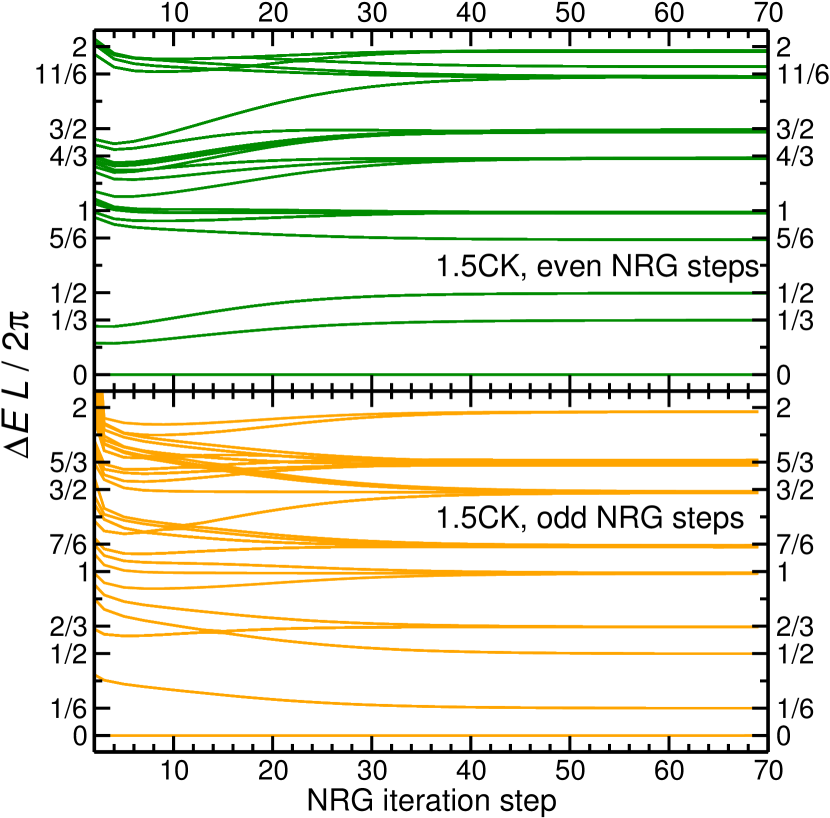
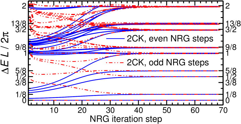
Figure 1: NRG flow and finite size excitation spectrum of the 1.5CK model (top) in comparison with the 2CK fixed point spectrum (bottom). $\Delta E$ stands for the excitation energy of the allowed energy levels and $L$ is the system size. The 1.5CK fixed point shows even-odd oscillation with the changing parity of the NRG iteration steps, whereas there is non such oscillation for the 2CK fixed point, and therefore the energy levels corresponding to iteration steps with differing parity could have been superimposed on each other without obscuring the figure. The ratio of the two distinct neighboring level spacings seen in the fixed point spectrums is  1:2  for the 1.5CK model, whereas it is  1:3  in the 2CK model and  1:1  in a Fermi liquid. (top) ${\cal H}_{\perp}^{1.5\textrm{C}\textrm{K}}+{\cal H}_{z}^{1.5\textrm{C}\textrm{K}}$ was solved at ${\cal J}=0.25D$ (in units of the bandwidth, $D$) with discretization parameter $\Lambda=2$ keeping at most 1000 states of the U(1) charge symmetry at each NRG step. (bottom) 2CK fixed point spectrum using the SU$(2)_{\textrm{s}pin}\times$SU$(2)_{\textrm{c}harge1}\times$SU$(2)_{\textrm{c}harge2}$ symmetry of the model while keeping at most 500 multiplets at each NRG step.

Energy spectrum of the 1.5CK model.

To confirm that both ${\cal H}_{\perp}^{1.5\textrm{C}\textrm{K}}$ and ${\cal H}_{\perp}^{1.5\textrm{C}\textrm{K}}+{\cal H}_{z}^{1.5\textrm{C}\textrm{K}}$ together with the kinetic energy of the conduction electrons indeed flow to a NFL fixed point, I solved them with NRG Wilson75 ; Toth08 . During the calculations I could make use of only the charge symmetry of these models, as they lack spin symmetry. I obtained the same, 1.5CK fixed point spectrum for both Hamiltonians. The NRG flow and the 1.5CK fixed point spectrum of ${\cal H}_{\perp}^{1.5\textrm{C}\textrm{K}}+{\cal H}_{z}^{1.5\textrm{C}\textrm{K}}$ for ${\cal J}=0.25$ in units of the bandwidth are shown in Fig. 1 next to the 2CK spectrum. The ratio of the two neighboring level spacings in the excitation spectrums is 1:2 for the 1.5CK model, whereas it is 1:3 in the 2CK model and 1:1 in a Fermi liquid. Thus, in this regard, the 1.5CK model is a more basic NFL quantum impurity model than the 2CK model. The 1.5CK fixed point spectrum shows even-odd oscillation due to particle-hole symmetry and that three more conduction electron creation operators are introduced in each NRG iteration step. That is the same argument that was applied in Wilson’s paper for the one-channel Kondo model Wilson75 . As expected, the physical properties computed around the 1.5CK fixed point cannot depend on the parity of the NRG iteration steps. This assertion was checked numerically for the specific heat. Presenting the thermodynamic and dynamic properties of the half-integer channel Kondo models using NRG will be the subject of a further study, just as extending conformal field theoretical (CFT) considerations Affleck91 to these models in order to understand their excitation spectrum and other properties. From e.g. the CFT solutions we know that in the 2CK model the electronic specific heat coefficient and the magnetic susceptibility both diverge as $\log T$ when $T\to 0$, whereas for higher channel numbers the divergence is faster as $T\to 0$. An intriguing question is whether the same considerations apply to the 1.5CK model, and how the divergence of these quantities is affected as $T\to 0$.

Conclusion.

I presented a family of NFL quantum impurity models where a spin-half impurity is exchange coupled to an odd number conduction electron species. Computing and understanding the physical properties of these models, and matching them with physical properties observed in materials are yet to follow.

References

- (1) H. R. Ott, H. Rudigier, Z. Fisk, and J. L. Smith, Phys. Rev. Lett. 50, 1595 (1983).
- (2) C. L. Seaman, M. B. Maple, B. W. Lee, S. Ghamaty, M. S. Torikachvili, J.-S. Kang, L. Z. Liu, J. W. Allen, and D. L. Cox, Phys. Rev. Lett. 67, 2882 (1991).
- (3) M. Suzuki, T. Murakami, Jpn. J. Appl. Phys. 26, L524 (1987).
- (4) M. Gurvitch, A. T. Fiory, Phys. Rev. Lett. 59, 1337 (1987).
- (5) D. L. Ginsberg, Physical Properties of High Temperature Superconductors I-V, World Scientific, Singapore (1989-96); K. H. Bennemann and J. B. Ketterson (Eds), Superconductivity: Vol. 1: Conventional and Unconventional Superconductors, Vol. 2: Novel Superconductors, Springer-Verlag Berlin Heidelberg (2008).
- (6) R. H. Liu et al., Phys. Rev. Lett. 101, 087001 (2008).
- (7) M. Gooch, B. Lv, B. Lorenz, A. M. Guloy, and Ch. W. Chu, Phys. Rev. B 79, 104504 (2009).
- (8) L. Fang et al., Phys. Rev. B 80, 140508(R) (2009).
- (9) S. Kasahara et al., Phys. Rev. B 81, 184519 (2010).
- (10) N. Stojilovic, A. Koncz, L. W. Kohlman, R. Hu, C. Petrovic, S. V. Dordevic, Phys. Rev. B 81, 174518 (2010).
- (11) P. B. Allen, R. M. Wentzcovitch, W. W. Schulz, P. C. Canfield, Phys. Rev. B 48, 4359 (1993).
- (12) M. M. Qazilbash, K. S. Burch, D. Whisler, D. Shrekenhamer, B. G. Chae, H. T. Kim, D. N. Basov, Phys. Rev. B 74, 205118 (2006).
- (13) P. Kostic, Y. Okada, N. C. Collins, Z. Schlesinger, J. W. Reiner, L. Klein, A. Kapitulnik, T. H. Geballe, M. R. Beasley, Phys. Rev. Lett. 81, 2498 (1998).
- (14) P. Khalifah, K. D. Nelson, R. Jin, Z. Q. Mao, Y. Liu, Q. Huang, X. P. A. Gao, A. P. Ramirez, R. J. Cava, Nature 411, 669 (2001).
- (15) Y. S. Lee, J. Yu, J. S. Lee, T. W. Noh, T.-H. Gimm, Han-Yong Choi, C. B. Eom, Phys. Rev. B 66, 041104(R) (2002).
- (16) S. Nakatsuji, Y. Machida, Y. Maeno, T. Tayama, T. Sakakibara, J. van Duijn, L. Balicas, J. N. Millican, R. T. Macaluso, J. Y. Chan, Phys. Rev. Lett. 96, 087204 (2006).
- (17) G. Cao, V. Durairaj, S. Chikara, L. E. DeLong, S. Parkin, P. Schlottmann, Phys. Rev. B 76, 100402(R) (2007).
- (18) C. Pfleiderer, S. R. Julian, G. G. Lonzarich, Nature 414, 427-430 (2001);
- (19) M. J. Steiner, F. Beckers, Ph. G. Niklowitz, G. G. Lonzarich, Physica B 329, 1079 (2003);
- (20) M. Brando, W. J. Duncan, D. Moroni-Klementowicz, C. Albrecht, D. Grüner, R. Ballou, F. M. Grosche, Phys. Rev. Lett. 101, 026401 (2008);
- (21) G. R. Stewart, Rev. Mod. Phys. 73, 797 (2001); ibid. 78, 743 (2006).
- (22) B. Dardel, D. Malterre, M. Grioni, P. Weibel, Y. Baer, J. Voit, D. Jérôme, Europhys. Lett. 24, 687 (1993);
- (23) J. Moser, M. Gabay, P. Auban-Senzier, D. Jérome, K. Bechgaard, J. M. Fabre, Eur. Phys. J. B 1, 39 (1998).
- (24) M. Bockrath, D. H. Cobden, J. Lu, A. G. Rinzler, R. E. Smalley, L. Balents, P. L. McEuen, Nature 397, 598-601 (1999).
- (25) N. Barišić, M. K. Chana, Y. Lie, G. Yua, X. Zhaoa, M. Dressel, A. Smontarac, M. Greven, Proc. Natl. Acad. Sci. U.S.A. 110, 12235 (2013).
- (26) Y. Li, V. Balédent, N. Barišić, Y. Cho, B. Fauqué, Y. Sidis, G. Yu1, X. Zhao, P. Bourges, M. Greven, Nature 455, 372 (2008).
- (27) S. I. Mirzaei et al., Proc. Natl. Acad. Sci. U.S.A. 110, 5774 (2013).
- (28) M. K. Chan, M. J. Veit, C. J. Dorow, Y. Ge, Y. Li, W. Tabis, Y. Tang, X. Zhao, N. Barišić, M. Greven, Phys. Rev. Lett. 113, 177005 (2014).
- (29) Y. Ando, S. Komiya, K. Segawa, S. Ono, Y. Kurita, Phys. Rev. Lett. 93, 267001 (2004).
- (30) T. R. Chien, Z. Z. Wang, N. P. Ong, Phys. Rev. Lett. 67, 2088 (1991); H. Y. Hwang, B. Batlogg, H. Takagi, H. L. Kao, J. Kwo, R. J. Cava, J. J. Krajewski, W. F. Peck, Jr., Phys. Rev. Lett. 72, 2636 (1994).
- (31) Z. Schlesinger, R. T. Collins, F. Holtzberg, C. Feild, S. H. Blanton, U. Welp, G. W. Crabtree, Y. Fang, J. Z. Liu, Phys. Rev. Lett. 65, 801 (1990).
- (32) G. Blumberg, M. V. Klein, K. Kadowaki, C. Kendziora, P. Guptasarma, D. Hinks, J. Phys. Chem. Solids 59, 1932 (1998).
- (33) C. Berthier, M. H. Julien, M. Horvatić, Y. Berthier, Journal de Physique I, 6, 2205 (1996).
- (34) R. W. Hill, C. Proust, L. Taillefer, P. Fournier, R. L. Greene, Nature 414, 711 (2001); C. Proust, K. Behnia, R. Bel, D. Maude, S. I. Vedeneev, Phys. Rev. B 72, 214511 (2005).
- (35) J. M. Harris, Y. F. Yan, P. Matl, N. P. Ong, P. W. Anderson, T. Kimura, K. Kitazawa, Phys. Rev. Lett. 75, 1391 (1995).
- (36) S. A. Grigera, R. S. Perry, A. J. Schofield, M. Chiao, S. R. Julian, G. G. Lonzarich, S. I. Ikeda, Y. Maeno, A. J. Millis, A. P. Mackenzie, Science 294, 329 (2001).
- (37) C. M. Varma, P. B. Littlewood, S. Schmitt-Rink, E. Abrahams, A. E. Ruckenstein, Phys. Rev. Lett. 63 1996 (1989).
- (38) E. Miranda, V. Dobrosavljević, Rep. Prog. Phys. 68, 2337 (2005).
- (39) S. Tomonaga, Prog. Theor. Phys. 5, 544 (1950); J. M. Luttinger, J. Math. Phys. 4, 1154 (1963).
- (40) Ph. Nozières, A. Blandin, J. Phys. Paris 41, 193 (1980).
- (41) A. Zawadowski, Phys. Rev. Lett. 45, 211 (1980).
- (42) K. G. Wilson, Rev. Mod. Phys. 47, 4 (1975).
- (43) D. M. Cragg, P. Lloyd, Ph. Nozières, J. Phys. C: Solid State Phys. 13, 803 (1980).
- (44) D. L. Cox, Phys. Rev. Lett. 59, 1240 (1987).
- (45) G. F. Koster, J. O. Dimmock, R. G. Wheeler, H. Statz, Properties of the Thirty-Two Point Groups, MIT Press, Cambridge, Massachusetts (1963).
- (46) A. I. Tóth, C. P. Moca, Ö. Legeza, and G. Zaránd, Phys. Rev. B 78, 245109 (2008).
- (47) I. Affleck, A. W. W. Ludwig, Nucl. Phys. B 352, 849 (1991).