The profile decomposition for the hyperbolic Schrödinger equation

Abstract.

In this note, we prove the profile decomposition for hyperbolic Schrödinger (or mixed signature) equations on $\mathbf{R}^{2}$ in two cases, one mass-supercritical and one mass-critical. First, as a warm up, we show that the profile decomposition works for the ${\dot{H}}^{\frac{1}{2}}$ critical problem. Then, we give the derivation of the profile decomposition in the mass-critical case based on an estimate of Rogers-Vargas [26].

1. Introduction

We will consider the hyperbolic (or mixed signature) Schrödinger equation on $\mathbf{R}^{2}$, which is given by

(1.1) $$i\partial_{t}u+\partial_{x}\partial_{y}u=|u|^{p}u,\hskip 14.22636ptu(x,y,0)=u_{0}(x,y).$$

In particular, we will focus on the cases $p=4$ and $p=2$. The case $p=2$ arises naturally in the study of modulation of wave trains in gravity water waves, see for instance [32, 34]; it is also a natural component of the Davey-Stewartson system [19, 30]. As can be observed quickly from the nature of the dispersion relation, the linear problem

(1.2) $$i\partial_{t}u+\partial_{x}\partial_{y}u=0,\hskip 14.22636ptu(x,y,0)=u_{0}(x,y).$$

satisfies the same Strichartz estimates and rather similar local smoothing estimates as its elliptic counterpart, the standard Schrödinger equation. In particular, there exists a constant $C<\infty$ such that

(1.3) $$\|e^{it\partial_{x}\partial_{y}}f\|_{L^{4}_{x,y,t}}\leq C\|f\|_{L^{2}_{x,y}}.$$

Hence, large data local in time well-posedness and global existence for small data with $p\geq 2$ can be observed using standard methods that can be found in classical texts such as [4, 30]. For quasilinear problems with mixed signature, some local well-posedness results have been developed recently, see [15, 23]. Non-existence of bound states was established in [11] and a class of bound states that are not in $L^{2}$ were constructed in [22].

Long time low regularity theory for this equation at large data remains unknown however. Recently, an approach to global existence for sufficiently regular solutions was taken in [33], but it is conjectured that (1.1) should have global well-posedness and scattering for all initial data in $L^{2}$. Much progress has been made recently in proving global well-posedness and scattering for various critical and supercritical dispersive equations by applying concentration compactness tools, which originated with the works of Lions [20, 21]. One major step in applying modern concentration compactness tools to dispersive equations is the profile decomposition, see [14, 17]. The idea is that given a small data global existence result, one proves that if the large data result is false then there is a critical value of norm of the initial data at which for instance a required integral fails to be finite. Then, the profile decomposition ensures that failure occurs because of an almost periodic critical element, which may then be analyzed further and in ideal settings ruled out completely. See [6, 7] and references therein for applications of this idea in the setting of focusing and defocusing Schrödinger equations for instance.

A major breakthrough in profile decompositions arose in the works of Gérard [10], Merle-Vega [24], Bahouri-Gérard [1], Gallagher [9] and Keraani [16]. Those results have then been used to understand how to prove results about scattering, blow-up and global well-posedness in many settings, see [17] for some examples. We also mention the recent work by Fanelli-Visciglia [8], where they consider profile decompositions in mass super-critical problems for a variety of operators, including (1.1).

As can be seen in [17, Section 4.4], the profile decomposition follows from refined bilinear Strichartz estimates. Using refined Strichartz estimates from [25] and bilinear Strichartz estimates, Bourgain [2] proved concentration estimates and global well-posedness in $H^{3/5+\epsilon}$ for the defocusing, cubic elliptic nonlinear Schrödinger equation in $\mathbf{R}^{2}$. Building on this work, Merle-Vega [24] proved a profile decomposition for the mass-critical elliptic nonlinear Schrödinger equation in two dimensions.

For the hyperbolic NLS, Lee, Vargas and Rogers-Vargas [18, 26, 35] have provided refined linear and bilinear estimates, drawing on results of Tao [31] for the elliptic Schrödinger equation. In particular [26] gives an improved Strichartz estimate similar to our Proposition 9 and uses it to prove lower bounds on concentration of mass at blow-up. An improved Strichartz estimate is also the key element in our profile decomposition, following the standard machinery described in [17, Section 4.4]. For completeness, we provide a proof of Proposition 9, which, although drawing on similar ideas as in [26], outlines more explicitly the additional orthogonality of rectangles with skewed ratios.

The major issue in following the standard proof of the profile decomposition is that the mixed signature nature of (1.1) means that an essential bilinear interaction estimate that holds in the elliptic case fails. This is compensated for in [35] by making a required orthogonality assumption for the refined bilinear Strichartz to hold (see the statement in Lemma 3 below). To overcome this difficulty, we use a double Whitney decomposition to precisely identify the right scales, which introduces many different rectangles that are controlled using the fact that functions with support on two rectangles of different aspect ratios have small bilinear interactions. We note that while we here focus on analysis in $2$ dimensions to keep the technical computations focused and directed, we expect many of the calculations to be generalizable to other dimensions as in [17].

The paper is structured as follows: in Section 2, we set up the problem, discuss some basic symmetries and establish some important bilinear estimates; in Section 3 we establish the result in the mass-supercritical case using the extra compactness that comes from the Sobolev embedding; in Section 4, we establish the main precise Strichartz estimate in the paper and in Section 5, we obtain the profile decomposition for the mass-critical problem and deduce the existence of a minimal blow-up solution. Finally, we conclude with a short Appendix in which we correct an error in the published version of this article.

Acknowledgments. The first author was supported in part by U.S. NSF Grant DMS - 1500424 The second author was supported in part by U.S. NSF Grants DMS–1312874 and DMS-1352353. The third author was supported in part by U.S. NSF Grant DMS–1558729 and a Sloane Research fellowship. The fourth author was supported in part by U.S. NSF Grant DMS-1516565. We wish to thank Andrea Nahmod, Klaus Widmayer, Daniel Tataru, Nathan Totz for helpful conversations during the production of this work. Part of this work was initiated when some of the authors were at the Hausdorff Research Institute for Mathematics in Bonn, then progressed during visits to the Institut des Hautes Études in Paris, the Mathematical Sciences Research Institute in Berkeley and the Institute for Mathematics and Applications in Minneapolis. The authors would like to thank these institutions for hosting subsets of them at various times in the last several years.

We thank also an anonymous referee who pointed out the results of Rogers-Vargas [26] and its relevance for this work and Emanuel Carneiro for pointing out that error in the original appendix and sharing his manuscript on optimizers for (1.3), [3].

2. Properties of (1.1)

Observe that a solution to

(2.1) $$i\partial_{t}u+\partial_{x}\partial_{y}u=|u|^{2}u,\hskip 14.22636ptu(x,y,t)=u_{0}(x,y),$$

has a number of symmetries:

1. Translation: for any $(x_{0},y_{0})\in\mathbf{R}^{2}$,

   (2.2) $$u(x,y,t)\mapsto u(x-x_{0},y-y_{0},t),$$

2. Modulation: for any $\theta\in\mathbf{R}$,

   (2.3) $$u(x,y,t)\mapsto e^{i\theta}u(x,y,t).$$

3. Scaling: for any $\lambda_{1},\lambda_{2}>0$,

   (2.4) $$u(x,y,t)\mapsto\sqrt{\lambda_{1}\lambda_{2}}u(\lambda_{1}x,\lambda_{2}y,\lambda_{1}\lambda_{2}t),$$

4. Galilean symmetry: for $(\xi_{1},\xi_{2})\in\mathbf{R}^{2}$,

   (2.5) $$u(x,y,t)\mapsto e^{-it\xi_{1}\xi_{2}}e^{i[x\xi_{1}+y\xi_{2}]}u(x-\xi_{1}t,y-\xi_{2}t,t).$$

5. Pseudo-conformal symmetry:

   (2.6) $$u(x,y,t)\mapsto\frac{e^{i\frac{xy}{t}}}{it}\overline{u}(\frac{x}{t},\frac{y}{t},\frac{1}{t}).$$

These symmetries all preserve the $L^{2}_{x,y}$ norm. The first two symmetries $\eqref{1.2}$-$\eqref{1.5}$, as well as the scaling symmetry properly redefined, also preserve the $\dot{H}_{h}^{s}$ norm for any $s\in\mathbf{R}$, where

$$\begin{split}\|f\|_{\dot{H}_{h}^{s}}^{2}&=\||\partial_{x}|^{\frac{s}{2}}|\partial_{y}|^{\frac{s}{2}}f\|_{L^{2}}^{2}.\end{split}$$

Note that this norm has similar scaling laws as the more usual $\dot{H}^{s}$ norm. Other examples of anisotropic equations have appeared in for instance [28, 13]. For example, for the $\dot{H}^{1/2}$ - critical problem

(2.7) $$i\partial_{t}u+\partial_{x}\partial_{y}u=|u|^{4}u,\hskip 14.22636ptu(x,y,0)=u_{0}(x,y),$$

the symmetries are thus:

1. Translation: for any $(x_{0},y_{0})\in\mathbf{R}^{2}$,

   (2.8) $$u(x,y,t)\mapsto u(x-x_{0},y-y_{0},t),$$

2. Scaling: for any $\lambda_{1},\lambda_{2}>0$,

   (2.9) $$u(x,y,t)\mapsto(\lambda_{1}\lambda_{2})^{1/4}u(\lambda_{1}x,\lambda_{2}y,\lambda_{1}\lambda_{2}t),$$

3. Modulation: for any $\theta\in\mathbf{R}$,

   (2.10) $$u(x,y,t)\mapsto e^{i\theta}u(x,y,t).$$

We will treat the profile decomposition for $\eqref{1.6}$ as a warm-up, before tackling the profile decomposition for the mass-critical problem $\eqref{1.1}$.

2.1. Notations

Let $\varphi$ be a usual smooth bump function such that $\varphi(x)=1$ when $|x|\leq 1$ and $\varphi(x)=0$ when $|x|\geq 2$. We also let

$$\psi(x)=\varphi(x)-\varphi(2x).$$

We will often consider various projections in Fourier space. Given a rectangle $R=R(c,\ell_{x},\ell_{y})$, centered at $c=(c_{x},c_{y})$ and with sides parallel to the axis of length $2\ell_{x}$ and $2\ell_{y}$, we define

(2.11) $$\begin{split}\varphi_{R}(x,y)=\varphi(\ell_{x}^{-1}(x-c_{x}))\varphi(\ell_{y}^{-1}(y-c_{y})).\end{split}$$

We define the operators

$$\begin{split}\widehat{Q_{M,N}f}(\xi,\eta)&=\psi(M^{-1}\xi)\psi(N^{-1}\eta)\widehat{f}(\xi,\eta),\\ \widehat{P_{R}f}(\xi,\eta)&=\varphi_{R}(\xi,\eta)\widehat{f}(\xi,\eta).\end{split}$$

The first operator is only sensitive to the scales involved, while the second also accounts for the location in Fourier space. We also let $|R|=4\ell_{x}\ell_{y}$ denote its area.

2.2. Some Preliminary Estimates

We start with a nonisotropic version of the Sobolev embedding.

Lemma 1.

There holds that

$$\|f\|_{L^{q}_{x,y}}\lesssim\||\partial_{x}|^{\frac{s}{2}}|\partial_{y}|^{\frac{s}{2}}f\|_{L^{p}_{x,y}}$$

whenever $1<p\leq q<\infty$, $0\leq s<1$ and

$$\frac{1}{q}=\frac{1}{p}-\frac{s}{2}$$

Proof of Lemma 1.

The proof, although easy, highlights the need to treat each direction independently. Using Sobolev embedding in $1d$, Minkowski inequality and Sobolev again, we obtain that

$$\begin{split}\|f\|_{L^{q}_{x}(\mathbf{R},L^{q}_{y}(\mathbf{R}))}&\lesssim\||\partial_{x}|^{\frac{s}{2}}f\|_{L^{q}_{y}(\mathbf{R},L^{p}_{x}(\mathbf{R}))}\lesssim\||\partial_{x}|^{\frac{s}{2}}f\|_{L^{p}_{x}(\mathbf{R},L^{q}_{y}(\mathbf{R}))}\\ &\lesssim\||\partial_{y}|^{\frac{s}{2}}|\partial_{x}|^{\frac{s}{2}}f\|_{L^{p}_{x,y}}\end{split}$$

which is what we wanted. ∎

We have two basic refinements of (1.3). Note the difference in orthogonality requirements between Lemma 2 and Lemma 3.

Lemma 2.

Assume that $f=P_{R_{1}}f$ and $g=P_{R_{2}}g$ where $R_{i}=R(c^{i},\ell_{x},\ell_{y})$ and $|c^{1}_{x}-c^{2}_{x}|=N\geq 4\ell_{x}$, and let $u$ (resp. $v$) be a solution of (1.2) with initial data $f$ (resp. $g$). Then

(2.12) $$\|uv\|_{L^{2}_{x,y,t}}\lesssim\left(\frac{\ell_{x}}{N}\right)^{\frac{1}{2}}\|f\|_{L^{2}_{x,y}}\|g\|_{L^{2}_{x,y}}.$$

Lemma 3.

Assume that $f=P_{R_{1}}f$ and $g=P_{R_{2}}g$ where $R_{i}=R(c^{i},\ell_{x},\ell_{y})$, $|c^{1}_{x}-c^{2}_{x}|\geq 4\ell_{x}$ and $|c^{1}_{y}-c^{2}_{y}|\geq 4\ell_{y}$, and let $u$ (resp. $v$) be a solution of (1.2) with initial data $f$ (resp. $g$). Then

$$\|uv\|_{L^{q}_{x,y,t}}\lesssim(\ell_{x}\ell_{y})^{1-\frac{2}{q}}\|f\|_{L^{2}_{x,y}}\|g\|_{L^{2}_{x,y}}$$

whenever $q>5/3$.

Lemma 3 is the main refined bilinear estimate and appears essentially in [35] when dealing with cubes. The result as stated here follows by scaling rectangles to cubes.

Proof of Lemma 2.

We simply write that

$$\begin{split}\widehat{u^{2}}(\xi,\eta,t)&=I(\xi,\eta,t),\\ I(\xi,\eta,t)&=\iint_{\mathbf{R}}e^{-it\omega}\varphi_{R_{1}}(\xi_{1},\eta_{1})\varphi_{R_{2}}(\xi-\xi_{1},\eta-\eta_{1})\\ &\hskip 56.9055pt\times\widehat{f}(\xi_{1},\eta_{1})\widehat{g}(\xi-\xi_{1},\eta-\eta_{1})d\xi_{1}d\eta_{1},\\ \omega&=\xi_{1}\eta_{1}+(\xi-\xi_{1})(\eta-\eta_{1})\end{split}$$

we may now change variable in the integral

(2.13) $$\begin{split}(\xi_{1},\eta_{1})\mapsto(\xi_{1},\omega),\qquad J:=\frac{\partial(\xi_{1},\omega)}{\partial(\xi_{1},\eta_{1})}=\begin{pmatrix}1&0\\ 2\eta_{1}-\eta&2\xi_{1}-\xi\end{pmatrix}\end{split}$$

and in particular, we remark that

(2.14) $$|J|=|(\xi-\xi_{1})-\xi_{1}|\simeq N,$$

so that

$$\begin{split}I(\xi,\eta,t)=&\iint_{\mathbf{R}}e^{-it\omega}\varphi_{R_{1}}(\xi_{1},\eta_{1})\varphi_{R_{2}}(\xi-\xi_{1},\eta-\eta_{1})\\ &\hskip 28.45274pt\times\widehat{f}(\xi_{1},\eta_{1})\widehat{g}(\xi-\xi_{1},\eta-\eta_{1})\cdot J^{-1}d\xi_{1}d\omega,\\ \eta_{1}&=\eta_{1}(\xi_{1},\omega;\xi,\eta).\\ \end{split}$$

Taking into consideration the Fourier transform in time and using Plancherel, followed by Cauchy-Schwarz, we find that

$$\begin{split}&\|I(\xi,\eta,\cdot)\|_{L^{2}_{t}}^{2}=\\ &\int_{\mathbf{R}}\left|\int_{\mathbf{R}}\varphi_{R_{1}}(\xi_{1},\eta_{1})\varphi_{R_{2}}(\xi-\xi_{1},\eta-\eta_{1})\widehat{f}(\xi_{1},\eta_{1})\widehat{g}(\xi-\xi_{1},\eta-\eta_{1})\cdot J^{-1}d\xi_{1}\right|^{2}d\omega\\ &\leq\sup_{\xi,\eta,\eta_{1}}\int_{\mathbf{R}}\varphi_{R_{1}}(\xi_{1},\eta_{1})\varphi_{R_{2}}(\xi-\xi_{1},\eta-\eta_{1})d\xi_{1}\times\\ &\quad\int_{\mathbf{R}}\int_{\mathbf{R}}\varphi_{R_{1}}(\xi_{1},\eta_{1})\varphi_{R_{2}}(\xi-\xi_{1},\eta-\eta_{1})\left|\widehat{f}(\xi_{1},\eta_{1})\widehat{g}(\xi-\xi_{1},\eta-\eta_{1})\right|^{2}\cdot J^{-2}d\xi_{1}d\omega.\\ \end{split}$$

Now, we use the fact that $R_{1}$ has width $\ell_{x}$, together with (2.14) to obtain, after undoing the change of variables, that

$$\begin{split}\|I(\xi,\eta,\cdot)\|_{L^{2}_{t}}^{2}&\lesssim\frac{\ell_{x}}{N}\int_{\mathbf{R}}\int_{\mathbf{R}}\varphi_{R_{1}}(\xi_{1},\eta_{1})\varphi_{R_{2}}(\xi-\xi_{1},\eta-\eta_{1})\\ &\hskip 56.9055pt\left|\widehat{f}(\xi_{1},\eta_{1})\widehat{g}(\xi-\xi_{1},\eta-\eta_{1})\right|^{2}\cdot J^{-1}d\xi_{1}d\omega\\ &\lesssim\frac{\ell_{x}}{N}\int_{\mathbf{R}}\int_{\mathbf{R}}\left|\widehat{f}(\xi_{1},\eta_{1})\widehat{g}(\xi-\xi_{1},\eta-\eta_{1})\right|^{2}d\xi_{1}d\eta_{1}.\\ \end{split}$$

Integrating with respect to $(\xi,\eta)$, we then obtain (2.12). ∎

We will in fact use the following consequence of Lemma 3.

Lemma 4.

Under the assumptions of Lemma 3, it holds that

(2.15) $$\|uv\|_{L^{\frac{40}{21}}_{x,y,t}}\lesssim(\ell_{x}\ell_{y})^{-\frac{3}{20}}\|\widehat{f}\|_{L^{\frac{20}{11}}_{x,y}}\|\widehat{g}\|_{L^{\frac{20}{11}}_{x,y}}.$$

Proof.

Indeed, using Lemma 3, we find that

$$\|e^{it\partial_{x}\partial_{y}}f\cdot e^{it\partial_{x}\partial_{y}}g\|_{L^{\frac{12}{7}}_{x,y,t}}\lesssim(\ell_{x}\ell_{y})^{-\frac{1}{6}}\|\widehat{f}\|_{L^{2}_{x,y}}\|\widehat{g}\|_{L^{2}_{x,y}},$$

while a crude estimate gives that

$$\begin{split}\|e^{it\partial_{x}\partial_{y}}f\cdot e^{it\partial_{x}\partial_{y}}g\|_{L^{\infty}_{x,y,t}}\lesssim\|\widehat{f}\|_{L^{1}_{x,y}}\|\widehat{g}\|_{L^{1}_{x,y}}.\end{split}$$

Interpolation gives (2.15). ∎

Another tool we will need in the profile decomposition is the following local smoothing result which is essentially equivalent to Lemma 2:

Lemma 5.

Let $\phi\in L^{2}_{x,y}$. There holds that

$$\begin{split}\sup_{x}\|Q_{M,N}e^{it\partial_{x}\partial_{y}}\phi(x,\cdot)\|_{L^{2}_{y,t}}&\lesssim N^{-\frac{1}{2}}\|\phi\|_{L^{2}_{x,y}},\\ \sup_{y}\|Q_{M,N}e^{it\partial_{x}\partial_{y}}\phi(\cdot,y)\|_{L^{2}_{x,t}}&\lesssim M^{-\frac{1}{2}}\|\phi\|_{L^{2}_{x,y}}.\\ \end{split}$$

Proof.

The proof is similar to the one in the elliptic case and follows from Plancherel after using a change of variable similar to (2.13). An equivalent statement with proof occurs in [19, Theorem $2.1$]. See also [5] for a general statement of Local Smoothing Estimates for Dispersive Equations. ∎

3. Mass-supercritical HNLS

In this section, we observe that $\dot{H}_{h}^{s}$ has similar improved Sobolev inequalities as the $\dot{H}^{1/2}$ Sobolev norm. A typical example is the following:

Lemma 6.

Let $f\in C^{\infty}_{c}(\mathbf{R}^{2})$. There holds that

(3.1) $$\begin{split}\|f\|_{L^{6}_{x,y}}&\lesssim\left(\sup_{M,N}(MN)^{-\frac{1}{6}}\|Q_{M,N}f\|_{L^{\infty}}\right)^{\frac{1}{3}}\|f\|_{\dot{H}_{h}^{\frac{2}{3}}}^{\frac{2}{3}}\lesssim\|f\|_{\dot{H}_{h}^{\frac{2}{3}}},\\ \end{split}$$

and consequently,

(3.2) $$\|f\|_{L^{4}_{x,y}}\lesssim\left(\sup_{M,N}(MN)^{-\frac{1}{4}}\|Q_{M,N}f\|_{L^{\infty}}\right)^{\frac{1}{6}}\|f\|_{\dot{H}_{h}^{\frac{1}{2}}}^{\frac{5}{6}}\lesssim\|f\|_{\dot{H}_{h}^{\frac{1}{2}}}.$$

This is essentially a consequence of the following simple inequalities

(3.3) $$\begin{split}\|Q_{M,N}f\|_{L^{\infty}_{x,y}}&\lesssim N^{\frac{1}{2}}\|Q_{M,N}f\|_{L^{\infty}_{x}L^{2}_{y}}\lesssim N^{\frac{1}{2}}\|Q_{M,N}f\|_{L^{2}_{y}L^{\infty}_{x}}\\ &\lesssim(MN)^{\frac{1}{2}}\|Q_{M,N}f\|_{L^{2}_{x,y}},\end{split}$$

and similarly after exchanging the role of $x$ and $y$.

Proof of Lemma 6:

Indeed, we may simply develop

$$\begin{split}\|f\|_{L^{6}_{x,y}}^{6}&\lesssim\sum_{\begin{subarray}{c}M_{1},\dots,M_{6},\\ N_{1},\dots,N_{6}\end{subarray}}\iint_{\mathbf{R}\times\mathbf{R}}Q_{M_{1},N_{1}}f\cdot Q_{M_{2},N_{2}}f\dots Q_{M_{6},N_{6}}fdxdy\end{split}$$

without loss of generality, we may assume that

$$\begin{split}M_{5},M_{6}\lesssim\mu_{2}=\max_{2}\{M_{1},M_{2},M_{3},M_{4}\},\\ N_{5},N_{6}\lesssim\nu_{2}=\max_{2}\{N_{1},N_{2},N_{3},N_{4}\},\\ \end{split}$$

where $\max_{2}(S)$ denotes the second largest element of the set $S$, and then using Hölder’s inequality and summing over $M_{5},M_{6}$ and $N_{5},N_{6}$, we obtain

$$\begin{split}&\|f\|_{L^{6}_{x,y}}^{6}\lesssim\left(\sup_{M,N}(MN)^{-\frac{1}{6}}\|Q_{M,N}f\|_{L^{\infty}}\right)^{2}\times\\ &\qquad\sum_{\begin{subarray}{c}M_{1},\dots,M_{4},\,\,M_{5},M_{6}\leq\mu_{2}\\ N_{1},\dots,N_{4},\,\,N_{5},N_{6}\leq\nu_{2}\end{subarray}}(M_{5}M_{6}N_{5}N_{6})^{\frac{1}{6}}\iint_{\mathbf{R}\times\mathbf{R}}|Q_{M_{1},N_{1}}f|\dots|Q_{M_{4},N_{4}}f|dxdy\\ &\lesssim\left(\sup_{M,N}(MN)^{-\frac{1}{6}}\|Q_{M,N}f\|_{L^{\infty}}\right)^{2}\times\\ &\hskip 56.9055pt\sum_{\begin{subarray}{c}M_{1},\dots,M_{4}\\ N_{1},\dots,N_{4}\end{subarray}}(\mu_{2}\nu_{2})^{\frac{1}{3}}\iint_{\mathbf{R}\times\mathbf{R}}|Q_{M_{1},N_{1}}f|\dots|Q_{M_{4},N_{4}}f|dxdy.\end{split}$$

Now, using (3.3) and estimating the norms corresponding to the two lower frequencies in each direction in $L^{\infty}$, and the two highest ones in $L^{2}$, one quickly finds that

$$\begin{split}\sum_{\begin{subarray}{c}M_{1},\dots,M_{4}\\ N_{1},\dots,N_{4}\end{subarray}}(\mu_{2}\nu_{2})^{\frac{1}{3}}\iint_{\mathbf{R}\times\mathbf{R}}|Q_{M_{1},N_{1}}f|\dots|Q_{M_{4},N_{4}}f|\,dxdy\lesssim\|f\|_{\dot{H}^{\frac{2}{3}}_{h}}^{4},\end{split}$$

which finishes the proof. Inequality (3.2) then follows by interpolation.

$\Box$

At this point, the usual profile decomposition follows easily from the following simple Lemma 7 below.

Lemma 7.

There exists $\delta>0$ such that

$$\|e^{it\partial_{x}\partial_{y}}f\|_{L^{8}_{x,y,t}}\lesssim\left(\sup_{M,N,t,x,y}(MN)^{-\frac{1}{4}}|\left(e^{it\partial_{x}\partial_{y}}Q_{M,N}f\right)(x,y)|\right)^{\delta}\|f\|_{\dot{H}^{\frac{1}{2}}_{h}}^{1-\delta}.$$

Proof of Lemma 7.

We use Hölder’s inequality, Sobolev embedding Lemma 1, Strichartz estimates and (3.2) to get for $u=e^{it\partial_{x}\partial_{y}}f$

$$\begin{split}\|u\|_{L^{8}_{x,y,t}}&\lesssim\|u\|_{L^{6}_{t}L^{12}_{x,y}}^{\frac{3}{4}}\|u\|_{L^{\infty}_{t}L^{4}_{x,y}}^{\frac{1}{4}}\\ &\lesssim\||\partial_{x}|^{\frac{1}{4}}|\partial_{y}|^{\frac{1}{4}}u\|_{L^{6}_{t}L^{3}_{x,y}}^{\frac{3}{4}}\cdot\left(\sup_{M,N,t}(MN)^{-\frac{1}{4}}\|Q_{M,N}u(t)\|_{L^{\infty}_{x,y}}\right)^{\frac{1}{24}}\|f\|_{\dot{H}^{\frac{1}{2}}_{h}}^{\frac{5}{24}}\\ &\lesssim\|f\|_{\dot{H}^{\frac{1}{2}}_{h}}^{\frac{23}{24}}\cdot\left(\sup_{M,N,t}(MN)^{-\frac{1}{4}}\|Q_{M,N}u(t)\|_{L^{\infty}_{x,y}}\right)^{\frac{1}{24}}.\end{split}$$

∎

3.1. The mass-supercritical profile decomposition

Let us take the group action on functions given by $g_{n}^{j}=g(x_{n}^{j},y_{n}^{j},\lambda_{1,n}^{j},\lambda_{2,n}^{j})$ such that

$$(g_{n}^{j})^{-1}f=(\lambda_{n,1}^{j}\lambda_{n,2}^{j})^{\frac{1}{4}}[f](\lambda_{n,1}^{j}x+x_{n}^{j},\lambda_{n,2}^{j}y+y_{n}^{j}).$$

We can now state the $\dot{H}^{\frac{1}{2}}_{h}$-profile decomposition for $(\ref{1.6})$.

Proposition 8.

Let $\|u_{n}\|_{\dot{H}^{\frac{1}{2}}_{h}}\leq A$ be a sequence that is bounded $\dot{H}^{\frac{1}{2}}_{h}$. Then possibly after passing to a subsequence, for any $1\leq j<\infty$ there exist $\phi^{j}\in\dot{H}^{\frac{1}{2}}_{h}$, $(t_{n}^{j},x_{n}^{j},y_{n}^{j})\in\mathbf{R}^{3}$, $\lambda_{n,1}^{j}$, $\lambda_{n,2}^{j}\in(0,\infty)$ such that for any $J$,

(3.4) $$u_{n}=\sum_{j=1}^{J}g_{n}^{j}e^{it_{n}^{j}\partial_{x}\partial_{y}}\phi^{j}+w_{n}^{J},$$

(3.5) $$\lim_{J\rightarrow\infty}\limsup_{n\rightarrow\infty}\|e^{it\partial_{x}\partial_{y}}w_{n}^{J}\|_{L_{x,y,t}^{8}}=0,$$

such that for any $1\leq j\leq J$,

(3.6) $$e^{-it_{n}^{j}\partial_{x}\partial_{y}}(g_{n}^{j})^{-1}w_{n}^{J}\rightharpoonup 0,$$

weakly in $\dot{H}^{\frac{1}{2}}_{h}$,

(3.7) $$\lim_{n\rightarrow\infty}\left(\|u_{n}\|_{\dot{H}^{\frac{1}{2}}_{h}}^{2}-\sum_{j=1}^{J}\|\phi^{j}\|_{\dot{H}^{\frac{1}{2}}_{h}}^{2}-\|w_{n}^{J}\|_{\dot{H}^{\frac{1}{2}}_{h}}^{2}\right)=0,$$

and for any $j\neq k$,

$$\limsup_{n\to\infty}\left[\left|\ln\left(\frac{\lambda_{n,1}^{j}}{\lambda_{n,1}^{k}}\right)\right|+\left|\ln\left(\frac{\lambda_{n,2}^{j}}{\lambda_{n,2}^{k}}\right)\right|+\frac{|x_{n}^{j}-x_{n}^{k}|}{(\lambda_{n,1}^{j}\lambda_{n,1}^{k})^{1/2}}+\frac{|y_{n}^{j}-y_{n}^{k}|}{(\lambda_{n,2}^{j}\lambda_{n,2}^{k})^{1/2}}\right.$$

$$\hskip 113.81102pt\left.+\frac{|t_{n}^{j}(\lambda_{n,1}^{j}\lambda_{n,2}^{j})-t_{n}^{k}(\lambda_{n,1}^{k}\lambda_{n,2}^{k})|}{(\lambda_{n,1}^{j}\lambda_{n,2}^{j}\lambda_{n,1}^{k}\lambda_{n,2}^{k})^{1/2}}\right]=\infty.$$

The proof of Proposition 8 of this follows by simple adaptation of the techniques in [17, Section 4.4], as originally introduced in [16]. We note that a similar statement also appears in works of Fanelli-Visciglia [8].

4. Profile decomposition for the mass-critical HLS

In this section, we focus on the mass-critical case. This case is more delicate for two reasons. First we need to account for the Galilean invariance symmetry in (2.5) and second, we cannot use a simple Sobolev estimate as in (3.2) to fix the frequency scales. We follow closely the work in [17, Section $4$] with a small variant in the use of modulation orthogonality and an additional argument for interactions of rectangles with skewed aspect ratios.

4.1. A precised Strichartz inequality

The main result in this section is the following proposition from which it is not hard to obtain a good profile decomposition. We need to introduce the norm

(4.1) $$\|\phi\|_{X_{p}}:=\left(\sum_{R\in\mathcal{R}}|R|^{-\frac{p}{20}}\|\phi\mathfrak{1}_{R}\|_{L^{\frac{20}{11}}}^{p}\right)^{\frac{1}{p}}$$

where $\mathcal{R}$ stands for the collection of all dyadic rectangles. That is, rectangles with both sides parallel to an axis, of possibly different dyadic size, whose center is a multiple of the same dyadic numbers, given by the form

(4.2) $$\begin{split}\mathcal{R}&:=\{R_{k,n,p,m}\,:\,k,n,m,p\in\mathbb{Z}\},\\ R_{k,n,p,m}&:=\{(x,y):\,\,n-1\leq 2^{-k}x\leq n+1,\,\,m-1\leq 2^{-p}y\leq m+1\}.\end{split}$$

Note in particular that these spaces are nested: $X_{p}\subset X_{q}$ whenever $p\leq q$. The motivation for the space $L^{\frac{20}{11}}$ in (4.1) can be motivated by the $X^{q}_{p}$ Strichartz estimate in Theorem $4.23$ from [17].

Proposition 9.

Let $\phi\in C^{\infty}_{c}(\mathbf{R}^{2})$, then, there holds that for all $p>2$,

(4.3) $$\|\phi\|_{X_{p}}\lesssim_{p}\|\phi\|_{L^{2}}$$

and in addition, there exists $p>2$ such that

(4.4) $$\|e^{it\partial_{x}\partial_{y}}\phi\|_{L^{4}_{x,y,t}}^{4}\lesssim\left(\sup_{R}|R|^{-\frac{1}{2}}\sup_{x,y,t}|e^{it\partial_{x}\partial_{y}}(P_{R}\phi)(x,y)|\right)^{\frac{4}{21}}\|\widehat{\phi}\|_{X_{p}}^{\frac{80}{21}}.$$

We refer to [26] for a different proof of a slightly stronger estimate. Let us first recall the Whitney decomposition.

Lemma 10 (Whitney decomposition).

There exists a tiling of the plane minus the diagonal

$$\begin{split}\mathbf{R}^{2}\setminus D&=\Cup I\times J,\qquad D=\{(x,x),\quad x\in\mathbf{R}\},\end{split}$$

made of dyadic intervals such that $|I|=|J|$ and

$$\begin{split}6|I|\leq\hbox{dist}(I\times J,D)\leq 24|I|.\end{split}$$

We will consider two independent Whitney decompositions of $\mathbf{R}\times\mathbf{R}$:

(4.5) $$\begin{split}1_{\{\mathbf{R}^{2}\times\mathbf{R}^{2}\setminus D\}}(\xi_{1},\eta_{1},\xi_{2},\eta_{2}):=\sum_{I_{1}\sim I_{2},\,\,J_{1}\sim J_{2}}\mathfrak{1}_{I_{1}}(\xi_{1})\mathfrak{1}_{J_{1}}(\eta_{1})\mathfrak{1}_{I_{2}}(\xi_{2})\mathfrak{1}_{J_{2}}(\eta_{2}),\end{split}$$

where $I_{i}$ and $J_{j}$ are dyadic intervals of $\mathbf{R}$ and $\sim$ is an equivalence relation such that, for each fixed $I$, there are only finitely many $J$’s such that $I\sim J$, uniformly in $I$ (i.e. equivalence classes have bounded cardinality) and if $I\sim J$, then $|I|=|J|$ and $\hbox{dist}(I,J)\simeq|I|$. We also extend the equivalence relation to rectangles in the following fashion:

$$I\times J\sim I^{\prime}\times J^{\prime}\qquad\text{if and only if}\qquad I\sim I^{\prime}\ \text{and}\ J\sim J^{\prime}.$$

We would like to follow the argument in [17] for the profile decomposition for the elliptic nonlinear Schrödinger equation. However, it is at this point where we reach the main technical obstruction to doing this. Recall that to estimate the $L_{x,y,t}^{2}$ norm of $[e^{it\Delta}f]^{2}$, it was possible to utilize Plancherel’s theorem, reducing the $L_{x,y,t}^{2}$ norm to an $l^{2}$ sum over pairs of Whitney squares.

This was because Plancherel’s theorem in frequency turned the sum over all pairs of equal area squares to an $l^{2}$ sum over squares centered at different points in frequency space, and then Plancherel’s theorem in time separated out pairs of squares with different area. Because there is only one square with a given area and center in space, this is enough. However, there are infinitely many rectangles with the same area and the same center. Thus, to reduce the $L_{x,y,t}^{2}$ norm of $[e^{it\partial_{x}\partial_{y}}f]^{2}$ to a $l^{2}$ sum over pairs of rectangles, that is rectangles whose sides obey the equivalence relation in both $x$ and $y$, it is necessary to deal with the off - diagonal terms, that is terms of the form

(4.6) $$\|[e^{it\partial_{x}\partial_{y}}P_{R_{1}}f][e^{it\partial_{x}\partial_{y}}P_{R_{2}}f][\overline{e^{it\partial_{x}\partial_{y}}P_{R_{1}^{\prime}}f}][\overline{e^{it\partial_{x}\partial_{y}}P_{R_{2}^{\prime}}f}]\|_{L_{x,y,t}^{1}},$$

where $R_{1}\sim R_{2}$ and $R_{1}^{\prime}\sim R_{2}^{\prime}$ are Whitney pairs of rectangles which have the same area, but very different dimensions in $x$ and $y$. In this case, Lemma 2 gives a clue with regard to how to proceed, since it leads to the generalized result that

(4.7) $$\|[e^{it\partial_{x}\partial_{y}}P_{R_{1}}f][\overline{e^{it\partial_{x}\partial_{y}}P_{R_{1}^{\prime}}f}]\|_{L_{x,y,t}^{2}}\ll\|P_{R_{1}}f\|_{L^{2}_{x,y}}\|P_{R_{1}^{\prime}}f\|_{L^{2}_{x,y}}.$$

Thus, it may be possible to sum the off diagonal terms. We will not use Lemma 2 specifically, but we will use the idea that rectangles of the same area but very different dimensions have very weak bilinear interactions.

Before we turn to the details, we first present the main orthogonality properties we will use. For simplicity of notation, given a dyadic rectangle $R$, let

$$\widehat{\phi_{R}}(x,y):=\widehat{\phi}(x,y)\mathfrak{1}_{R}(x,y)\qquad\hbox{ and }\qquad u_{R}(x,y,t):=\left(e^{it\partial_{x}\partial_{y}}\phi_{R}\right)(x,y)$$

and set $u=e^{it\partial_{x}\partial_{y}}\phi$. Also we will consider rectangles $R_{1}=I_{1}\times J_{1}$, $R_{2}=I_{2}\times J_{2}$, $R_{1}^{\prime}=I_{1}^{\prime}\times J_{1}^{\prime}$, $R_{2}^{\prime}=I_{2}^{\prime}\times J_{2}^{\prime}$.

Proceeding with the above philosophy in mind, using (4.5), we have that

$$\begin{split}\|u\|_{L^{4}_{x,y,t}}^{4}&=\|u^{2}\|_{L^{2}_{x,y,t}}^{2}=\|\sum_{R_{1}\sim R_{2}}u_{R_{1}}\cdot u_{R_{2}}\|_{L^{2}_{x,y,t}}^{2}\\ &=\|\sum_{\Omega}\sum_{\begin{subarray}{c}R_{1}\sim R_{2},\\ |R_{1}|=|R_{2}|=\Omega\end{subarray}}u_{R_{1}}\cdot u_{R_{2}}\|_{L^{2}_{x,y,t}}^{2}=\|\sum_{\Omega}I_{\Omega}\|_{L^{2}_{x,y,t}}^{2}.\end{split}$$

Using the polarization identity for a quadratic form,

$$Q(x_{1},y_{1})+Q(x_{2},y_{2})=\frac{1}{2}\left[Q(x_{1}+x_{2},y_{1}+y_{2})+Q(x_{1}-x_{2},y_{1}-y_{2})\right],$$

we compute that

$$\begin{split}e^{i\frac{t}{2}\xi\eta}\widehat{I_{\Omega}}&(\xi,\eta,t)=\sum_{\begin{subarray}{c}R_{1}\sim R_{2},\\ |R_{1}|=|R_{2}|=\Omega\end{subarray}}\int_{\mathbf{R}^{4}}\mathfrak{1}_{R_{1}}(\xi_{1},\eta_{1})\mathfrak{1}_{R_{2}}(\xi_{2},\eta_{2})e^{-i\frac{t}{2}(\xi_{1}-\xi_{2})(\eta_{1}-\eta_{2})}\\ &\times\widehat{f}(\xi_{1},\eta_{1})\widehat{f}(\xi_{2},\eta_{2})\delta(\xi-\xi_{1}-\xi_{2})\delta(\eta-\eta_{1}-\eta_{2})d\xi_{1}d\xi_{2}d\eta_{1}d\eta_{2}.\end{split}$$

Now we observe that since

$$|I_{1}|=|I_{2}|\simeq\hbox{dist}(I_{1},I_{2}),\qquad|J_{1}|=|J_{2}|\simeq\hbox{dist}(J_{1},J_{2}),$$

it holds that, on the support of integration,

$$|(\xi_{1}-\xi_{2})(\eta_{1}-\eta_{2})|\simeq|I_{1}|\cdot|J_{1}|\simeq\Omega.$$

Therefore, we have the following orthogonality in time

$$\|\sum_{\Omega}\widehat{I_{\Omega}}(\xi,\eta,\cdot)\|_{L^{2}_{t}}^{2}=\|e^{i\frac{t}{2}\xi\eta}\sum_{\Omega}\widehat{I_{\Omega}}(\xi,\eta,\cdot)\|_{L^{2}_{t}}^{2}\lesssim\sum_{\Omega}\|\widehat{I_{\Omega}}(\xi,\eta,\cdot)\|_{L^{2}_{t}}^{2}.$$

To continue, we need to control $I_{\Omega}$ uniformly in $\Omega$. We write that

$$\begin{split}\mathcal{I}_{\Omega}&=\left\|\sum_{\begin{subarray}{c}R_{1}\sim R_{2},\\ |R_{1}|=|R_{2}|=\Omega\end{subarray}}u_{R_{1}}\cdot u_{R_{2}}\right\|_{L^{2}_{x,y,t}}^{2}\\ &=\sum_{\begin{subarray}{c}R_{1}\sim R_{2},\,\,R_{1}^{\prime}\sim R_{2}^{\prime},\\ |R_{1}|=|R_{2}|=|R_{1}^{\prime}|=|R_{2}^{\prime}|=\Omega\end{subarray}}\int_{\mathbf{R}^{3}_{x,y,t}}u_{R_{1}}\cdot u_{R_{2}}\cdot\overline{u_{R_{1}^{\prime}}\cdot u_{R_{2}^{\prime}}}\,\,dxdydt\\ &=\sum_{\begin{subarray}{c}R_{1}\sim R_{2},\,\,R_{1}^{\prime}\sim R_{2}^{\prime}\\ |R_{1}|=|R_{2}|=|R_{1}^{\prime}|=|R_{2}^{\prime}|=\Omega\end{subarray}}\mathcal{I}_{R_{1}\sim R_{2},R_{1}^{\prime}\sim R_{2}^{\prime}}.\end{split}$$

To any rectangle $R=I\times J$, we associate its center $c=(c_{x},c_{y})$ and its scales $\ell_{x}(R)=|I|$ and $\ell_{y}(R)=|J|=\Omega/|I|$. For 2 rectangles $R$ and $R^{\prime}$ of equal area, we define their relative discrepancy by

$$\delta(R,R^{\prime})=\min\{\ell_{x}(R)/\ell_{x}(R^{\prime}),\ell_{y}(R)/\ell_{y}(R^{\prime})\}.$$

We want to decompose $\mathcal{I}_{\Omega}$ according to the discrepancy of $R_{1}=I_{1}\times J_{1}$ and $R_{1}^{\prime}=I_{1}^{\prime}\times J_{1}^{\prime}$. Using scaling relation (2.9), we may assume that $\Omega=1$, $\ell_{x}(R_{1})=\ell_{x}(R_{2})=1$ and that $\ell_{x}(R_{1}^{\prime})\leq\ell_{y}(R_{1}^{\prime})$, so that $R_{1}^{\prime}$ is a $\delta\times\delta^{-1}$ rectangle, where $\delta=\delta(R_{1},R_{1}^{\prime})$.

We first notice that, if $\mathcal{I}_{R_{1}\sim R_{2},R_{1}^{\prime}\sim R_{2}^{\prime}}\neq 0$, we must have that

(4.8) $$\begin{split}|c_{x}(R_{1})-c_{x}(R_{1}^{\prime})|&\,\,\lesssim\,\,\ell_{x}(R_{1})+\ell_{x}(R_{1}^{\prime}),\\ |c_{y}(R_{1})-c_{y}(R_{1}^{\prime})|&\,\,\lesssim\,\,\ell_{y}(R_{1})+\ell_{y}(R_{1}^{\prime}).\end{split}$$

and therefore, for any fixed $R_{1}$ and $\delta\gtrsim 1$, there can be only a bounded number of choices for $R_{1}^{\prime}$, so that

$$\begin{split}\mathcal{I}_{1}&\lesssim\sum_{\begin{subarray}{c}R_{1}\sim R_{2},\\ |R_{1}|=|R_{2}|=1\end{subarray}}\|u_{R_{1}}u_{R_{2}}\|_{L^{2}_{x,y,t}}^{2}.\end{split}$$

At this stage, we are in a similar position as in the elliptic case and we may follow the proof in [17, Section 4.4]. From now on, we will focus on the case $\delta\ll 1$.

In the case $\delta\ll 1$, we may in fact strengthen (4.8). Indeed for $\mathcal{I}_{R_{1}\sim R_{2},R_{1}^{\prime}\sim R_{2}^{\prime}}$ to be different from $0$, we must have that

(4.9) $$\begin{split}|c_{x}(R_{1})-c_{x}(R_{1}^{\prime})|&\,\,\simeq\,\,\ell_{x}(R_{1})+\ell_{x}(R_{1}^{\prime}),\\ |c_{y}(R_{1})-c_{y}(R_{1}^{\prime})|&\,\,\simeq\,\,\ell_{y}(R_{1})+\ell_{y}(R_{1}^{\prime}).\end{split}$$

This follows from the fact that (say)

$$\begin{split}&c_{x}(R_{1})+c_{x}(R_{2})-c_{x}(R_{1}^{\prime})-c_{x}(R_{2}^{\prime})\\ =&2\left[c_{x}(R_{1})-c_{x}(R_{1}^{\prime})\right]-\left[c_{x}(R_{1})-c_{x}(R_{2})\right]+\left[c_{x}(R_{1}^{\prime})-c_{x}(R_{2}^{\prime})\right],\end{split}$$

and the last bracket is bounded by $24\delta$, while the second to last is bounded below by $6$; however, for $\mathcal{I}_{R_{1}\sim R_{2},R_{1}^{\prime}\sim R_{2}^{\prime}}$ to be nonzero, there must exists $(\xi_{1},\xi_{2},\xi_{1}^{\prime},\xi_{2}^{\prime})\in R_{1}\times R_{2}\times R_{1}^{\prime}\times R_{2}^{\prime}$ such that

$$\begin{split}&\xi_{1}+\xi_{2}-\xi_{1}^{\prime}-\xi_{2}^{\prime}=0\qquad\hbox{and}\\ &|(\xi_{1}+\xi_{2}-\xi_{1}^{\prime}-\xi_{2}^{\prime})-(c_{x}(R_{1})+c_{x}(R_{2})-c_{x}(R_{1}^{\prime})-c_{x}(R_{2}^{\prime}))|\leq 2+2\delta.\end{split}$$

We will keep note of this by writing $R_{1}\simeq R_{1}^{\prime}$ (or sometimes $c(R_{1})\simeq c(R_{1}^{\prime})$) whenever (4.9) holds for rectangles of equal area.

Recall that $R_{1}^{\prime}$ is a $\delta\times\delta^{-1}$ rectangle; we can decompose all rectangles into $\delta\times 1$ rectangles. We may then partition

(4.10) $$\begin{split}R_{1}&=\bigcup_{a=1}^{\delta^{-1}}I_{1,a}\times J_{1}=\bigcup_{a=1}^{\delta^{-1}}R_{1,a},\qquad R_{2}=\bigcup_{\widetilde{a}=1}^{\delta^{-1}}I_{2,\widetilde{a}}\times J_{2}=\bigcup_{\widetilde{a}=1}^{\delta^{-1}}R_{2,\widetilde{a}},\\ R_{1}^{\prime}&=\bigcup_{b=1}^{\delta^{-1}}I_{1}^{\prime}\times J_{1,b}^{\prime}=\bigcup_{b=1}^{\delta^{-1}}R_{1,b}^{\prime},\qquad R_{2}^{\prime}=\bigcup_{\widetilde{b}=1}^{\delta^{-1}}I_{2}^{\prime}\times J_{2,\widetilde{b}}^{\prime}=\bigcup_{\widetilde{b}=1}^{\delta^{-1}}R_{2,\widetilde{b}}^{\prime}\end{split}$$

and by orthogonality, we see that

$$\begin{split}\mathcal{I}_{R_{1}\sim R_{2},R_{1}^{\prime}\sim R_{2}^{\prime}}&=\sum_{a\sim\widetilde{a},\,\,b\sim\widetilde{b}}\mathcal{I}_{R_{1,a}\sim R_{2,\widetilde{a}},R_{1,b}^{\prime}\sim R_{2,\widetilde{b}}^{\prime}}\end{split}$$

where

$$a\sim\widetilde{a}\qquad\text{if and only if}\qquad|c_{x}(R_{1,a})+c_{x}(R_{2,\widetilde{a}})-c_{x}(R_{1}^{\prime})-c_{x}(R_{2}^{\prime})|\lesssim\delta$$

and comparably in $y$ for $b\sim\widetilde{b}$. Thus, for fixed $R_{1}$, $R_{2}$, $R_{1}^{\prime}$ $R_{2}^{\prime}$, this gives two equivalence relations with $O(\delta^{-1})$ equivalence classes of (uniformly) bounded cardinality.

And proceeding as in (4.9), we can easily see that

(4.11) $$\begin{split}|c_{x}(R_{1,a})-c_{x}(R^{\prime}_{1,b})|\gtrsim 1,\qquad|c_{y}(R_{1,a})-c_{y}(R^{\prime}_{1,b})|\gtrsim\delta^{-1},\\ |c_{x}(R_{2,\widetilde{a}})-c_{x}(R^{\prime}_{2,\widetilde{b}})|\gtrsim 1,\qquad|c_{y}(R^{\prime}_{1,\widetilde{a}})-c_{y}(R^{\prime}_{2,\widetilde{b}})|\gtrsim\delta^{-1}.\end{split}$$

At this point, we have extracted all the orthogonality we need and we are ready to proceed with the proof of Proposition 9.

4.2. Proof of (4.4)

Using rescaling, we may assume that

(4.12) $$1=\sup_{R}|R|^{-\frac{1}{2}}\|e^{it\partial_{x}\partial_{y}}\phi_{R}\|_{L^{\infty}_{x,y,t}}.$$

From the considerations above, we obtain the expression

(4.13) $$\begin{split}\|e^{it\partial_{x}\partial_{y}}\phi\|_{L^{4}_{x,y,t}}^{4}&\lesssim\sum_{\Omega}\sum_{\begin{subarray}{c}R_{1}\sim R_{2},\,R_{1}^{\prime}\sim R_{2}^{\prime},\\ |R_{1}|=|R_{2}|=|R_{1}^{\prime}|=|R_{2}^{\prime}|=\Omega\end{subarray}}\mathcal{I}_{R_{1}\sim R_{2},R_{1}^{\prime}\sim R_{2}^{\prime}},\\ \end{split}$$

where the rectangles satisfy the condition (4.9). In addition, for fixed rectangles $R_{1}\sim R_{2}$, $R_{1}^{\prime}\sim R_{2}^{\prime}$ of equal area $\Omega$, let $\delta=\delta(R_{1},R_{1}^{\prime})$. As explained above, for fixed $\delta=\delta_{0}=O(1)$, we are in a position similar to the elliptic case and we may follow [17] to get

$$\begin{split}&\sum_{\Omega}\sum_{\begin{subarray}{c}R_{1}\sim R_{2},\,R_{1}^{\prime}\sim R_{2}^{\prime},\\ |R_{1}|=|R_{2}|=|R_{1}^{\prime}|=|R_{2}^{\prime}|=\Omega,\\ \delta(R_{1},R_{1}^{\prime})=\delta_{0}\end{subarray}}|\mathcal{I}_{R_{1}\sim R_{2},R_{1}^{\prime}\sim R_{2}^{\prime}}|\\ \lesssim&\sum_{\Omega}\sum_{\begin{subarray}{c}R_{1}\sim R_{2},\\ |R_{1}|=|R_{2}|=\Omega\end{subarray}}\|u_{R_{1}}u_{R_{2}}\|_{L^{2}_{x,y,t}}^{2}\\ \lesssim&\left(\sup_{R}|R|^{-\frac{1}{2}}\|u_{R}\|_{L^{\infty}_{x,y,t}}\right)^{\frac{4}{21}}\sum_{\begin{subarray}{c}R_{1}\sim R_{2}\end{subarray}}|R_{1}|^{\frac{2}{21}}\|u_{R_{1}}u_{R_{2}}\|_{L^{\frac{40}{21}}_{x,y,t}}^{\frac{40}{21}}\\ \lesssim&\sum_{\begin{subarray}{c}R_{1}\sim R_{2}\end{subarray}}\left\{|R_{1}|^{-\frac{1}{20}}\|\widehat{\phi_{R_{1}}}\|_{L^{\frac{20}{11}}_{x,y}}\cdot|R_{2}|^{-\frac{1}{20}}\|\widehat{\phi_{R_{2}}}\|_{L^{\frac{20}{21}}_{x,y,t}}\right\}^{\frac{40}{21}},\end{split}$$

where we have used Cauchy-Schwarz in the first inequality, Hölder’s inequality in the second and (4.12) together with Lemma 4 in the last inequality. This gives a bounded contribution as in (4.4) for any $p\leq 80/21$.

We need to adjust the above scheme when $\delta\ll 1$. In the following, we let

$$T_{\ll 1}:=\sum_{\delta\ll 1}\sum_{\Omega}\sum_{\begin{subarray}{c}R_{1}\sim R_{2},\,R_{1}^{\prime}\sim R_{2}^{\prime},\\ |R_{1}|=|R_{2}|=|R_{1}^{\prime}|=|R_{2}^{\prime}|=\Omega,\\ \delta(R_{1},R_{1}^{\prime})=\delta\end{subarray}}|\mathcal{I}_{R_{1}\sim R_{2},R_{1}^{\prime}\sim R_{2}^{\prime}}|\\$$

and to conclude the proof of (4.4), we need to prove that, for some $p>2$,

(4.14) $$T_{\ll 1}\lesssim\|\phi\|_{X_{p}}^{\frac{80}{21}}.$$

We can now use the finer decomposition (4.10) to write

$$\begin{split}\mathcal{I}_{R_{1}\sim R_{2},R_{1}^{\prime}\sim R_{2}^{\prime}}&=\sum_{a\sim\widetilde{a},\,b\sim\widetilde{b}}\mathcal{I}_{R_{1,a}\sim R_{2,\widetilde{a}},R_{1,b}^{\prime}\sim R_{2,\widetilde{b}}^{\prime}}\end{split}$$

where the new rectangles satisfy (4.11). Using Cauchy-Schwartz, then Hölder’s inequality with (4.12), we have that

$$\begin{split}|\mathcal{I}_{R_{1,a}\sim R_{2,\widetilde{a}},R_{1,b}^{\prime}\sim R_{2,\widetilde{b}}^{\prime}}|&\lesssim\|u_{R_{1,a}}\cdot u_{R^{\prime}_{1,b}}\|_{L^{2}_{x,y,t}}\cdot\|u_{R_{2,\widetilde{a}}}\cdot u_{R^{\prime}_{2,\widetilde{b}}}\|_{L^{2}_{x,y,t}}\\ &\lesssim(\delta\Omega)^{\frac{2}{21}}\|u_{R_{1,a}}\cdot u_{R^{\prime}_{1,b}}\|_{L^{\frac{40}{21}}_{x,y,t}}^{\frac{20}{21}}\cdot\|u_{R_{2,\widetilde{a}}}\cdot u_{R^{\prime}_{2,\widetilde{b}}}\|_{L^{\frac{40}{21}}_{x,y,t}}^{\frac{20}{21}}.\end{split}$$

Now, using Lemma 4 with (4.11), we obtain that

$$\begin{split}&|\mathcal{I}_{R_{1,a}\sim R_{2,\widetilde{a}},R_{1,b}^{\prime}\sim R_{2,\widetilde{b}}^{\prime}}|\\ \lesssim&(\delta\Omega)^{\frac{2}{21}}\cdot(\delta^{-1}\Omega)^{-\frac{6}{21}}\|\widehat{\phi_{R_{1,a}}}\|_{L^{\frac{20}{11}}_{x,y}}^{\frac{20}{21}}\|\widehat{\phi_{R_{2,\widetilde{a}}}}\|_{L^{\frac{20}{11}}_{x,y}}^{\frac{20}{21}}\|\widehat{\phi_{R^{\prime}_{1,b}}}\|_{L^{\frac{20}{11}}_{x,y}}^{\frac{20}{21}}\|\widehat{\phi_{R^{\prime}_{2,\widetilde{b}}}}\|_{L^{\frac{20}{11}}_{x,y}}^{\frac{20}{21}}.\end{split}$$

Since $20/11<40/21$ and since for fixed $a$, there are only a bounded number $\widetilde{a}$ such that $a\sim\widetilde{a}$, we can sum over $a$ to get

$$\begin{split}\sum_{a\sim\widetilde{a}}\|\widehat{\phi_{R_{1,a}}}\|_{L^{\frac{20}{11}}_{x,y}}^{\frac{20}{21}}\|\widehat{\phi_{R_{2,\widetilde{a}}}}\|_{L^{\frac{20}{11}}_{x,y}}^{\frac{20}{21}}&\lesssim\|\widehat{\phi_{R_{1}}}\|_{L^{\frac{20}{11}}_{x,y}}^{\frac{20}{21}}\|\widehat{\phi_{R_{2}}}\|_{L^{\frac{20}{11}}_{x,y}}^{\frac{20}{21}}\end{split}$$

and similarly for $b$, so that

(4.15) $$\begin{split}|\mathcal{I}_{R_{1}\sim R_{2},R_{1}^{\prime}\sim R_{2}^{\prime}}|&\lesssim\delta^{\frac{8}{21}}\Omega^{-\frac{4}{21}}\|\widehat{\phi_{R_{1}}}\|_{L^{\frac{20}{11}}_{x,y}}^{\frac{20}{21}}\|\widehat{\phi_{R_{2}}}\|_{L^{\frac{20}{11}}_{x,y}}^{\frac{20}{21}}\|\widehat{\phi_{R_{1}^{\prime}}}\|_{L^{\frac{20}{11}}_{x,y}}^{\frac{20}{21}}\|\widehat{\phi_{R_{2}^{\prime}}}\|_{L^{\frac{20}{11}}_{x,y}}^{\frac{20}{21}}.\end{split}$$

In addition, for rectangles of fixed areas and sizes $|R_{1}|=|R_{2}|=|R_{1}^{\prime}|=|R_{2}^{\prime}|$, $\ell_{x}(R_{1})=\ell_{x}(R_{2})$, $\ell_{x}(R_{1}^{\prime})=\ell_{x}(R_{2}^{\prime})$ also satisfying (4.9), we may use Cauchy Schwartz in the summation over the centers to get

$$\begin{split}\sum_{\begin{subarray}{c}R_{1}\sim R_{2},\\ R_{1}^{\prime}\sim R_{2}^{\prime}\end{subarray}}\|\widehat{\phi_{R_{1}}}\|_{L^{\frac{20}{11}}_{x,y}}^{\frac{20}{21}}\|\widehat{\phi_{R_{2}}}\|_{L^{\frac{20}{11}}_{x,y}}^{\frac{20}{21}}\|\widehat{\phi_{R_{1}^{\prime}}}\|_{L^{\frac{20}{11}}_{x,y}}^{\frac{20}{21}}\|\widehat{\phi_{R_{2}^{\prime}}}\|_{L^{\frac{20}{11}}_{x,y}}^{\frac{20}{21}}&\lesssim\sum_{R_{1}\simeq R_{1}^{\prime}}\|\widehat{\phi_{R_{1}}}\|_{L^{\frac{20}{11}}_{x,y}}^{\frac{40}{21}}\|\widehat{\phi_{R_{1}^{\prime}}}\|_{L^{\frac{20}{11}}_{x,y}}^{\frac{40}{21}}\end{split}$$

where the sum is taken over all rectangles $R_{1}\simeq R_{1}^{\prime}$ of the given sizes satisfying (4.9).

We can now get back to (4.14) and use (4.15) and the inequality above to get

$$\begin{split}T_{\ll 1}&\lesssim\sum_{\Omega}\sum_{A}\sum_{\delta\leq 1}\delta^{\frac{8}{21}}\Omega^{-\frac{4}{21}}\cdot\sum_{c_{1}\simeq c_{1}^{\prime}}\|\widehat{\phi_{R_{1}}}\|_{L^{\frac{20}{11}}_{x,y}}^{\frac{40}{21}}\|\widehat{\phi_{R_{1}^{\prime}}}\|_{L^{\frac{20}{11}}_{x,y}}^{\frac{40}{21}},\end{split}$$

where we have parameterized the lengths of the rectangles by $\Omega=|R_{1}|=|R_{1}^{\prime}|$, $A=\ell_{x}(R_{1})$ and $\delta=\ell_{x}(R_{1}^{\prime})/\ell_{x}(R_{1})$, and their centers by $c_{1}$, $c_{1}^{\prime}$.

Now for any $p>2$ choose $0<\theta(p)<1$ such that

(4.16) $$\frac{2\theta}{p}+\frac{1-\theta}{p}=\frac{21}{40}.$$

and observe that $\theta(p)\searrow\frac{1}{20}$ as $p\searrow 2$. Then by interpolation,

$$\begin{split}&\sum_{\begin{subarray}{c}\Omega,A,\\ c_{1}\simeq c_{1}^{\prime}\end{subarray}}\Omega^{-\frac{4}{21}}\|\widehat{\phi_{R_{1}}}\|_{L^{\frac{20}{11}}_{x,y}}^{\frac{40}{21}}\|\widehat{\phi_{R_{1}^{\prime}}}\|_{L^{\frac{20}{11}}_{x,y}}^{\frac{40}{21}}\\ \lesssim&\left(\sum_{\begin{subarray}{c}\Omega,A,\\ c_{1}\simeq c_{1}^{\prime}\end{subarray}}\Omega^{-\frac{p}{10}}\|\widehat{\phi_{R_{1}}}\|_{L^{\frac{20}{11}}_{x,y}}^{p}\|\widehat{\phi_{R_{1}^{\prime}}}\|_{L^{\frac{20}{11}}_{x,y}}^{p}\right)^{\frac{40}{21}\frac{1-\theta}{p}}\left(\sum_{\begin{subarray}{c}\Omega,A,\\ c_{1}\simeq c_{1}^{\prime}\end{subarray}}\Omega^{-\frac{p}{20}}\|\widehat{\phi_{R_{1}}}\|_{L^{\frac{20}{11}}_{x,y}}^{\frac{p}{2}}\|\widehat{\phi_{R_{1}^{\prime}}}\|_{L^{\frac{20}{11}}_{x,y}}^{\frac{p}{2}}\right)^{\frac{40}{21}\frac{2\theta}{p}}.\end{split}$$

Now, on the one hand, we observe that for a fixed choice of scales ($\Omega$, $A$ and $\delta$) and for each fixed $c_{1}$, there are at most $O(\delta^{-1})$ choices of $c_{1}^{\prime}$ satisfying (4.9) so we obtain that

(4.17) $$\begin{split}\sum_{\begin{subarray}{c}\Omega,A,\\ c_{1}\simeq c_{1}^{\prime}\end{subarray}}\Omega^{-\frac{p}{20}}\|\widehat{\phi_{R_{1}}}\|_{L^{\frac{20}{11}}_{x,y}}^{\frac{p}{2}}\|\widehat{\phi_{R_{1}^{\prime}}}\|_{L^{\frac{20}{11}}_{x,y}}^{\frac{p}{2}}&\lesssim\delta^{-1}\sum_{\begin{subarray}{c}\Omega,A,c_{1}\end{subarray}}\Omega^{-\frac{p}{20}}\|\widehat{\phi_{R_{1}}}\|_{L^{\frac{20}{11}}_{x,y}}^{p}\end{split}$$

and the other sum can be handled in an easier way: using Hölder’s inequality and forgetting about the relationship $c_{1}\simeq c_{1}^{\prime}$, we obtain that

(4.18) $$\begin{split}&\sum_{\Omega}\sum_{A}\sum_{c_{1}\simeq c_{1}^{\prime}}\Omega^{-\frac{p}{10}}\|\widehat{\phi_{R_{1}}}\|_{L^{\frac{20}{11}}_{x,y}}^{p}\|\widehat{\phi_{R_{1}^{\prime}}}\|_{L^{\frac{20}{11}}_{x,y}}^{p}\\ \lesssim&\sum_{\Omega}\sum_{A}\left(\sum_{c_{1}}\left\{\Omega^{-\frac{1}{20}}\|\widehat{\phi_{R_{1}}}\|_{L^{\frac{20}{11}}_{x,y}}\right\}^{p}\right)\cdot\left(\sum_{c_{1}^{\prime}}\left\{\Omega^{-\frac{1}{20}}\|\widehat{\phi_{R_{1}^{\prime}}}\|_{L^{\frac{20}{11}}_{x,y}}\right\}^{p}\right)\\ \lesssim&\left(\sum_{R}|R|^{-\frac{p}{20}}\|\widehat{\phi_{R}}\|_{L^{\frac{20}{11}}_{x,y}}^{p}\right)^{2}.\end{split}$$

Recall the definition (4.1). Combining (4.17) and (4.18), we obtain

$$\begin{split}T_{\ll 1}&\lesssim\sum_{\delta\leq 1}\delta^{\frac{8}{21}}\cdot\left(\delta^{-1}\|\widehat{\phi}\|_{X_{p}}^{p}\right)^{\frac{80}{21}\frac{\theta}{p}}\left(\|\widehat{\phi}\|_{X_{p}}^{2p}\right)^{\frac{40}{21}\frac{1-\theta}{p}}\lesssim\sum_{\delta\leq 1}\delta^{\frac{8}{21}(1-\frac{10\theta}{p})}\|\widehat{\phi}\|_{X_{p}}^{\frac{80}{21}}\end{split}$$

and this is summable in $\delta$ for $2<p<40/17$ small enough. The proof of (4.4) is thus complete and it remains to prove (4.3) which we now turn to.

4.3. Proof of (4.3)

We first state and prove the following simple result we will need in the proof.

Lemma 11.

Let $\mathcal{D}$ denote the set of dyadic intervals (on $\mathbf{R}$) and let $p>2$. For any $g\in C^{\infty}_{c}(\mathbf{R})$, there holds that

(4.19) $$\sum_{I\in\mathcal{D}}|I|^{-\frac{p}{20}}\|g\mathfrak{1}_{I}\|_{L^{\frac{20}{11}}_{x}}^{p}\lesssim\|g\|_{L^{2}_{x}}^{p}.$$

Proof of Lemma 11.

We may assume that $\|g\|_{L^{2}_{x}}=1$. For fixed $A$, we let $\mathcal{D}_{A}$ denote the set of dyadic intervals of length $A$ and we decompose

$$\begin{split}g=g^{+}+g^{-},\qquad g^{+}(x)=g(x)\mathfrak{1}_{\{|g(x)|>A^{-\frac{1}{2}}\}},\qquad g^{-}(x)=g(x)\mathfrak{1}_{\{|g(x)|\leq A^{-\frac{1}{2}}\}}.\end{split}$$

On the one hand, using that $\ell^{\frac{20}{11}}\subset\ell^{p}$,

$$\begin{split}\sum_{A}\sum_{I\in\mathcal{D}_{A}}|I|^{-\frac{p}{20}}\|g^{+}\mathfrak{1}_{I}\|_{L^{\frac{20}{11}}_{x}}^{p}&\lesssim\left(\sum_{A}A^{-\frac{1}{11}}\sum_{I\in\mathcal{D}_{A}}\|g^{+}\mathfrak{1}_{I}\|_{L^{\frac{20}{11}}_{x}}^{\frac{20}{11}}\right)^{\frac{11}{20}p}\\ &\lesssim\left(\sum_{A}A^{-\frac{1}{11}}\int_{\mathbf{R}}|g|^{\frac{20}{11}}\mathfrak{1}_{\{|g(x)|>A^{-\frac{1}{2}}\}}dx\right)^{\frac{11}{20}p}\\ &\lesssim\left(\int_{\mathbf{R}}|g|^{\frac{20}{11}}\cdot\left(\sum_{A>|g(x)|^{-2}}A^{-\frac{1}{11}}\right)dx\right)^{\frac{11}{20}p}\lesssim 1,\end{split}$$

while, for the other sum, we use Hölder’s inequality to get

$$\begin{split}\sum_{A}\sum_{I\in\mathcal{D}_{A}}A^{-\frac{p}{20}}\|g^{-}\mathfrak{1}_{I}\|_{L^{\frac{20}{11}}_{x}}^{p}&\lesssim\sum_{A}\sum_{I\in\mathcal{D}_{A}}A^{-\frac{p}{20}}\|g^{-}\mathfrak{1}_{I}\|_{L^{p}}^{p}\cdot|I|^{(\frac{11}{20}-\frac{1}{p})p}\\ &\lesssim\int_{\mathbf{R}}|g(x)|^{p}\cdot\sum_{\{A<|g(x)|^{-2}\}}A^{\frac{p-2}{2}}dx\\ &\lesssim\int_{\mathbf{R}}|g(x)|^{2}dx\lesssim 1\end{split}$$

and the proof is complete. ∎

Now, we proceed to prove (4.3).

Proof of (4.3).

Recall $\mathcal{D}$ stand for the set of dyadic intervals and $\mathcal{D}_{A}$ for the set of dyadic intervals of length $A$. We want to prove that

$$\begin{split}\sum_{I\in\mathcal{D}}|I|^{-\frac{p}{20}}\sum_{J\in\mathcal{D}}|J|^{-\frac{p}{20}}\|f\mathfrak{1}_{I\times J}\|_{L^{\frac{20}{11}}_{x,y}}^{p}\lesssim\|f\|_{L^{2}_{x,y}}^{p}.\end{split}$$

We claim that, for any fixed interval $I$,

(4.20) $$\sum_{J\in\mathcal{D}}|J|^{-\frac{p}{20}}\|f\mathfrak{1}_{I\times J}\|_{L^{\frac{20}{11}}_{x,y}}^{p}\lesssim\|f\mathfrak{1}_{I\times\mathbf{R}}\|_{L^{\frac{20}{11}}_{x}L^{2}_{y}}^{p}.$$

Once this is proved, we may simply apply Lemma 11 to the function

$$g(x):=\|f(x,\cdot)\|_{L^{2}_{y}}$$

to finish the proof.

From now on $I$ denotes a fixed interval and $f$ is a function supported on $\{x\in I\}$, i.e. $f=f\mathfrak{1}_{I\times\mathbf{R}}$. The proof of (4.20) is a small variation on the proof of Lemma 11. Fix a dyadic number $B$ and let

$$c_{B}=c_{B}(x)=B^{-\frac{1}{2}}\|f(x,\cdot)\|_{L^{2}_{y}}$$

and decompose accordingly

$$f=f^{+}+f^{-},\quad f^{+}=f\mathfrak{1}_{\{|f(x,y)|>c_{B}(x)\}},\quad f^{-}=f\mathfrak{1}_{\{|f(x,y)|\leq c_{B}(x)\}}.$$

We then compute that

$$\begin{split}&\sum_{B}\sum_{J\in\mathcal{D}_{B}}B^{-\frac{p}{20}}\|f^{+}\mathfrak{1}_{I\times J}\|_{L^{\frac{20}{11}}_{x,y}}^{p}\lesssim\left(\sum_{B}\sum_{J\in\mathcal{D}_{B}}B^{-\frac{1}{11}}\|f^{+}\mathfrak{1}_{I\times J}\|_{L^{\frac{20}{11}}_{x,y}}^{\frac{20}{11}}\right)^{\frac{11}{20}p}\\ &\hskip 56.9055pt\lesssim\left(\sum_{B}B^{-\frac{1}{11}}\int_{I_{x}}\int_{\mathbf{R}_{y}}|f^{+}|^{\frac{20}{11}}dy\,dx\right)^{\frac{11}{20}p}\\ &\hskip 56.9055pt\lesssim\left(\int_{I_{x}}\int_{\mathbf{R}_{y}}|f^{+}|^{\frac{20}{11}}\cdot\sum_{\{B:|f(x,y)|\geq c_{B}(x)\}}B^{-\frac{1}{11}}dy\,dx\right)^{\frac{11}{20}p}\\ &\hskip 56.9055pt\lesssim\left(\int_{I_{x}}\int_{\mathbf{R}_{y}}|f(x,y)|^{\frac{20}{11}}\cdot\left(\frac{|f(x,y)|}{\|f(x,\cdot)\|_{L^{2}_{y}}}\right)^{\frac{2}{11}}dy\,dx\right)^{\frac{11}{20}p}\\ &\hskip 56.9055pt\lesssim\left(\int_{I_{x}}\|f(x,\cdot)\|_{L^{2}_{y}}^{-\frac{2}{11}}\int_{\mathbf{R}_{y}}|f(x,y)|^{2}dy\,dx\right)^{\frac{11}{20}p}\\ &\hskip 56.9055pt\lesssim\|f\|_{L^{\frac{20}{11}}_{x}L^{2}_{y}}^{p},\end{split}$$

in the penultimate line, we note that though there is a negative power of the $L^{2}_{y}$ norm, the product of the two quantities is well-defined, especially as we can assume $f\in C^{\infty}_{c}$. Also, we have used the embedding $\ell^{1}\subset\ell^{\frac{11}{20}p}$ in the first inequality, the fact that dyadic intervals of a fixed length tile $\mathbf{R}$ in the second inequality, and we have summed a geometric series in the fourth inequality. Now for the second part, we compute that

$$\begin{split}\sum_{B}\sum_{J\in\mathcal{D}_{B}}&B^{-\frac{p}{20}}\|f^{-}\mathfrak{1}_{I\times J}\|_{L^{\frac{20}{11}}_{x,y}}^{p}\lesssim\sum_{B}\sum_{J\in\mathcal{D}_{B}}B^{-\frac{p}{20}}B^{p(\frac{11}{20}-\frac{1}{p})}\|f^{-}\mathfrak{1}_{I\times J}\|_{L^{p}_{y}(J:L^{\frac{20}{11}}_{x}(I))}^{p}\\ &\lesssim\sum_{B}B^{\frac{p-2}{2}}\int_{\mathbf{R}_{y}}\left(\int_{I_{x}}|f^{-}(x,y)|^{\frac{20}{11}}dx\right)^{\frac{11}{20}p}dy\\ &\lesssim\int_{\mathbf{R}_{y}}\sum_{B}\left(B^{\frac{p-2}{2}\frac{20}{11}\frac{1}{p}}\int_{I_{x}}|f^{-}(x,y)|^{\frac{20}{11}}dx\right)^{\frac{11}{20}p}dy\\ &\lesssim\int_{\mathbf{R}_{y}}\left(\int_{I_{x}}\sum_{B}B^{\frac{p-2}{p}\frac{10}{11}}|f^{-}(x,y)|^{\frac{20}{11}}dx\right)^{\frac{11}{20}p}dy,\end{split}$$

where we have used Hölder’s inequality in the first line and the inclusion $\ell^{1}\subset\ell^{\frac{11}{20}p}$ in the fourth line. Now, since $f^{-}$ is supported where

$$B\leq\left(\frac{\|f(x,\cdot)\|_{L^{2}_{y}}}{|f(x,y)|}\right)^{2},$$

summing in $B$ gives

$$\begin{split}&\sum_{B}\sum_{J\in\mathcal{D}_{B}}B^{-\frac{p}{20}}\|f^{-}\mathfrak{1}_{I\times J}\|_{L^{\frac{20}{11}}_{x,y}}^{p}\\ \lesssim&\int_{\mathbf{R}_{y}}\left(\int_{I_{x}}\|f(x,\cdot)\|_{L^{2}_{y}}^{\frac{20}{11}\frac{p-2}{p}}|f^{-}(x,y)|^{\frac{20}{11}\frac{2}{p}}dx\right)^{\frac{11}{20}p}dy.\end{split}$$

Using Minkowski inequality on the function

$$h(x,y)=\|f(x,\cdot)\|_{L^{2}_{y}}^{\frac{20}{11}\frac{p-2}{p}}|f^{-}(x,y)|^{\frac{20}{11}\frac{2}{p}},$$

we obtain

$$\begin{split}&\sum_{B}\sum_{J\in\mathcal{D}_{B}}B^{-\frac{p}{20}}\|f^{-}\mathfrak{1}_{I\times J}\|_{L^{\frac{20}{11}}_{x,y}}^{p}\\ \lesssim&\left(\int_{I_{x}}\left(\int_{\mathbf{R}_{y}}h^{\frac{11}{20}p}dy\right)^{\frac{20}{11}\frac{1}{p}}dx\right)^{\frac{11}{20}p}\\ \lesssim&\left(\int_{I_{x}}\left(\int_{\mathbf{R}_{y}}|f(x,y)|^{2}dy\right)^{\frac{20}{11}\frac{1}{p}}\|f(x,\cdot)\|_{L^{2}_{y}}^{\frac{20}{11}\frac{p-2}{p}}dx\right)^{\frac{11}{20}p}\\ \lesssim&\left(\int_{I_{x}}\|f(x,\cdot)\|_{L^{2}_{y}}^{\frac{20}{11}}dx\right)^{\frac{11}{20}p},\end{split}$$

which proves (4.20). Thus the proof is complete.

∎

5. The Profile Decomposition and Applications

The profile decomposition then follows from Proposition 9 in the usual way following the techniques in the proof of Theorems $4.25$ (the Inverse Strichartz Inequality) and $4.26$ (Mass Critical Profile Decomposition) from [17], for instance. We note that it is the proof of the Inverse Strichartz Inequality that requires the local smoothing estimates as in Lemma 5 to establish pointwise a.e. convergence of profiles to an element of $L^{2}_{x,y}$ through compactness considerations, otherwise the proof follows mutatis mutandis. Once the Inverse Strichartz Inequality is established, the proof of the Profile Decomposition follows verbatim.

Suppose $g_{n}^{j}=g(x_{n}^{j},y_{n}^{j},\lambda_{1,n}^{j},\lambda_{2,n}^{j},\xi_{n}^{j})$ is the group whose action on functions is given by

$$(g_{n}^{j})^{-1}f=(\lambda_{n,1}^{j}\lambda_{n,2}^{j})^{1/2}e^{-i\xi_{n,1}^{j}(\lambda_{n,1}^{j}x+x_{n}^{j})}e^{-i\xi_{n,2}^{j}(\lambda_{n,2}^{j}x+y_{n}^{j})}$$

$$\hskip 71.13188pt\times[f_{n}](\lambda_{n,1}^{j}x+x_{n}^{j},\lambda_{n,2}^{j}y+y_{n}^{j}).$$

The profile decomposition gives the following.

Theorem 12.

Let $\|u_{n}\|_{L^{2}_{x,y}(\mathbf{R}^{2})}\leq A$ be a sequence that is bounded $L^{2}_{x,y}(\mathbf{R}^{2})$. Then possibly after passing to a subsequence, for any $1\leq j<\infty$ there exist $\phi^{j}\in L^{2}_{x,y}(\mathbf{R}^{2})$, $(t_{n}^{j},x_{n}^{j},y_{n}^{j})\in\mathbf{R}^{3}$, $\xi_{n}^{j}\in\mathbf{R}^{2}$, $\lambda_{n,1}^{j}$, $\lambda_{n,2}^{j}\in(0,\infty)$ such that for any $J$,

(5.1) $$u_{n}=\sum_{j=1}^{J}g_{n}^{j}e^{it_{n}^{j}\partial_{x}\partial_{y}}\phi^{j}+w_{n}^{J},$$

(5.2) $$\lim_{J\rightarrow\infty}\limsup_{n\rightarrow\infty}\|e^{it\partial_{x}\partial_{y}}w_{n}^{J}\|_{L_{x,y,t}^{4}}=0,$$

such that for any $1\leq j\leq J$,

(5.3) $$e^{-it_{n}^{j}\partial_{x}\partial_{y}}(g_{n}^{j})^{-1}w_{n}^{J}\rightharpoonup 0,$$

weakly in $L^{2}_{x,y}(\mathbf{R}^{2})$,

(5.4) $$\lim_{n\rightarrow\infty}\left(\|u_{n}\|_{L^{2}_{x,y}}^{2}-\sum_{j=1}^{J}\|\phi^{j}\|_{L^{2}_{x,y}}^{2}-\|w_{n}^{J}\|_{L^{2}_{x,y}}^{2}\right)=0,$$

and for any $j\neq k$,

(5.5) $$\begin{split}&\lim_{n\rightarrow\infty}\left[\left|\ln\left(\frac{\lambda_{n,1}^{j}}{\lambda_{n,1}^{k}}\right)\right|+\left|\ln\left(\frac{\lambda_{n,2}^{j}}{\lambda_{n,2}^{k}}\right)\right|+\frac{|t_{n}^{j}(\lambda_{n,1}^{j}\lambda_{n,2}^{j})-t_{n}^{k}(\lambda_{n,1}^{k}\lambda_{n,2}^{k})|}{(\lambda_{n,1}^{j}\lambda_{n,2}^{j}\lambda_{n,1}^{k}\lambda_{n,2}^{k})^{1/2}}\right.\\ &\hskip 28.45274pt+(\lambda_{n,1}^{j}\lambda_{n,1}^{k})^{1/2}|\xi_{n,1}^{j}-\xi_{n,1}^{k}|+(\lambda_{n,2}^{j}\lambda_{n,2}^{k})^{1/2}|\xi_{n,2}^{j}-\xi_{n,2}^{k}|\\ &\hskip 56.9055pt+\frac{|x_{n}^{j}-x_{n}^{k}-2t_{n}^{j}(\lambda_{n,1}^{j}\lambda_{n,2}^{j})(\xi_{n,1}^{j}-\xi_{n,1}^{k})|}{(\lambda_{n,1}^{j}\lambda_{n,1}^{k})^{1/2}}\\ &\left.\hskip 56.9055pt+\frac{|y_{n}^{j}-y_{n}^{k}-2t_{n}^{j}(\lambda_{n,1}^{j}\lambda_{n,2}^{j})(\xi_{n,2}^{j}-\xi_{n,2}^{k})|}{(\lambda_{n,2}^{j}\lambda_{n,2}^{k})^{1/2}}\right]=\infty.\end{split}$$

5.1. Minimal mass blow-up solutions

As an application of the profile decomposition, we turn to a calculation that for instance originated in [16, 24]. Namely we construct a minimal mass solution to (2.1) which is a solution $u$ of minimal mass such that there exists a time $T^{*}$ such that

$$\int_{-T^{*}}^{T^{*}}\int_{\mathbf{R}^{2}_{x,y}}|u|^{4}\,dxdydt=+\infty.$$

In other words, it is a solution of least mass for which the small data global argument fails.

It turns out that if $u$ is a minimal mass blowup solution to $\eqref{1.1}$ then $u$ lies in a compact subset of $L^{2}_{x,y}(\mathbf{R}^{2})$ modulo the symmetry group $g$; more precisely, following [17, Chapter $5$, Theorem $5.2$], we can establish the following theorem.

Theorem 13.

Suppose $u$ is a minimal mass blowup solution to $(\ref{1.1})$ on a maximal time interval $I$ that blows up in both time directions. That is, $I$ is an open interval and for any $t_{0}\in I$,

(5.6) $$\int_{t_{0}}^{\sup(I)}\int|u(x,y,t)|^{4}dxdydt,\hskip 14.22636pt\int_{\inf(I)}^{t_{0}}\int|u(x,y,t)|^{4}dxdydt=\infty.$$

Then there exist $\lambda_{1},\lambda_{2}:I\rightarrow(0,\infty)$, $\widetilde{\xi}:I\rightarrow\mathbf{R}^{2}$, $\widetilde{x},\widetilde{y}:I\rightarrow\mathbf{R}$, such that for any $\eta>0$ there exists $C(\eta)<\infty$ such that

(5.7) $$\int_{|x-\widetilde{x}(t)|>\frac{C(\eta)}{\lambda_{1}(t)}}|u(x,y,t)|^{2}dxdy+\int_{|y-\widetilde{y}(t)|>\frac{C(\eta)}{\lambda_{2}(t)}}|u(x,y,t)|^{2}dxdy$$

$$+\int_{|\xi_{1}-\widetilde{\xi}_{1}(t)|>C(\eta)\lambda_{1}(t)}|\hat{u}(\xi,t)|^{2}d\xi+\int_{|\xi_{2}-\widetilde{\xi}_{2}(t)|>C(\eta)\lambda_{2}(t)}|\hat{u}(\xi,t)|^{2}d\xi<\eta.$$

Proof.

Take a sequence $t_{n}\in I$. Then conservation of mass implies that after passing to a subsequence we may make a profile decomposition of $u(t_{n})=u_{n}$. If there exists $j$ such that, along a subsequence, $t_{n}^{j}\rightarrow\pm\infty$, say $t_{n}^{j}\rightarrow\infty$, then

(5.8) $$\lim_{n\rightarrow\infty}\|e^{it\partial_{x}\partial_{y}}(g_{n}^{j}e^{it_{n}^{j}\partial_{x}\partial_{y}}\phi^{j})\|_{L_{x,y,t}^{4}([0,\infty)\times\mathbf{R}^{2})}=0,$$

so combining perturbative arguments, $(\ref{decouple})$, and the fact that $u$ is a blowup solution with minimal mass then $u$ scatters forward in time to a free solution. Thus, we may assume that for each $j$, $t_{n}^{j}$ converges to some $t^{j}\in\mathbf{R}$. Then taking $e^{it^{j}\partial_{x}\partial_{y}}\phi^{j}$ to be the new $\phi^{j}$, we may assume that each $t_{n}^{j}=0$.

Now suppose that

(5.9) $$\sup_{j}\|\phi^{j}\|_{L^{2}_{x,y}(\mathbf{R}^{2})}<\|u(t)\|_{L^{2}_{x,y}(\mathbf{R}^{2})}.$$

Then if $v^{j}$ is the solution to $\eqref{1.1}$ with initial data $\phi^{j}$, since $\|u(t)\|_{L^{2}}$ is the minimal mass for blowup to occur, each $v^{j}$ scatters both forward and backward in time, with

(5.10) $$\|v^{j}\|_{L_{x,y,t}^{4}(\mathbf{R}\times\mathbf{R}^{2})}^{2}\lesssim\|\phi^{j}\|_{L^{2}_{x,y}}^{2}<\infty,\qquad\hbox{uniformly in }j.$$

Then if $v_{n}^{j}$ is the solution to $\eqref{1.1}$ with initial data $g_{n}^{j}\phi^{j}$, $v_{n}^{j}=g_{n}^{j}(v^{j}((\lambda_{n,1}^{j}\lambda_{n,2}^{j})^{-1}t))$. We note that, for $v$ either a profile $v_{n}^{\ell}$ or the remainder $w_{n}^{J}$,

(5.11) $$\|v_{n}^{j}v_{n}^{k}v\|_{L_{x,y,t}^{\frac{4}{3}}}\leq\|v_{n}^{j}v_{n}^{k}\|_{L^{2}_{x,y,t}}\|v\|_{L^{4}_{x,y,t}}.$$

In addition, $\|v\|_{L^{4}_{x,y,t}}$ remains bounded either by (5.10) (for $v_{n}^{\ell}$) or as a consequence of the small data theory and (5.2) (for $w_{n}^{J}$).

By approximation by compactly supported functions, it is easy to see that, if $j\neq k$,

(5.12) $$\|v_{n}^{j}v_{n}^{k}\|_{L^{2}_{x,y,t}}\to 0$$

when $n\rightarrow\infty$ as a consequence of (5.5).

As a result, using simple perturbation theory, we obtain that, for $J$ large enough,

$$\begin{split}\|u(t_{n}+t)-\sum_{j=1}^{J}v_{n}^{j}(t)\|_{L^{4}_{x,y,t}}\lesssim 1\end{split}$$

and using again (5.11)-(5.12), we obtain that

$$\begin{split}\|\sum_{j=1}^{J}v_{n}^{j}(t)\|_{L^{4}_{x,y,t}}^{4}\lesssim\sum_{j=1}^{J}\|v_{n}^{j}\|_{L^{4}_{x,y,t}}^{4}\lesssim\sum_{j=1}^{J}\|\phi^{j}\|_{L^{2}_{x,y}}^{2}<\infty.\end{split}$$

which, together with (5.4) contradicts (5.6).

Thus, after reordering we should have $\|\phi^{1}\|_{L^{2}_{x,y}}=\|u(t)\|_{L^{2}_{x,y}}$ and $\phi^{j}=0$ for any $j\geq 2$. But this holds if and only if $u(t)$ lies in a set $GK$, where $G$ is the group generated by $g_{n}^{j}$ and $K$ is a compact set in $L^{2}$. This completes the proof of the theorem. ∎

Appendix A Extremizers for Strichartz Estimates for (1.2)

We end with a few considerations on extremizers for the Strichartz inequality (1.3), that is functions $f$ of unit $L^{2}_{x,y}$-norm and constant $\overline{C}$ such that

(A.1) $$\begin{split}\|e^{it\partial_{x}\partial_{y}}f\|_{L^{4}_{x,y,t}}=\overline{C}:=\sup\{\|e^{it\partial_{x}\partial_{y}}g\|_{L^{4}_{x,y,t}}:\,\,\|g\|_{L^{2}_{x,y}}=1\}.\\ \end{split}$$

The original version of this paper stated erroneously that Gaussians were optimizers for the Strichartz norm above, and gave a corresponding numerical value for $\overline{C}$. In fact, it was later proved in [3] that Gaussians are not critical points of the Strichartz norm and thus cannot be optimizers. One can however use the profile decomposition for Theorem 12 to prove existence of an extremizer (see [29] for a similar proof).

Proposition 14.

There exists $f\in L^{2}_{x,y}(\mathbf{R}^{2})$ such that

(A.2) $$\|e^{it\partial_{x}\partial_{y}}f\|_{L^{4}_{x,y,t}}=\overline{C}\|f\|_{L^{2}_{x,y}}.$$

where $\overline{C}$ is given in (A.1).

The exact nature of the extremizer $f$ above remains mysterious. Preliminary numerical investigations confirm that the optimizer should be a genuine function of $x$ and $y$ and suggests that it has nice decay and smoothness properties.

We reproduce some plots of the amplitude of an extremizer and its Fourier transform below. These are obtained by maximizing the Strichartz norm among functions in the span of the first $25$ Hermite functions with unit $L^{2}$ norm. Some care has been given to obtain accurate computations and minimize boundary effects, but we do not mean that the result is anything but suggestive. However, it seems to indicate that extremizers are indeed smooth and localized and that they can be chosen real valued, which is why we have not reproduced their phase.

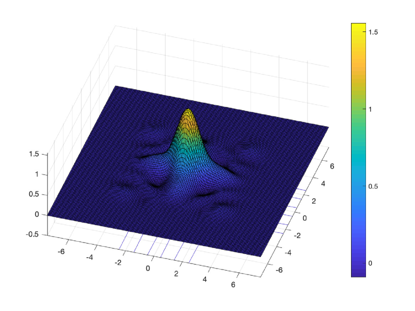
(a) Plot of $|f|$

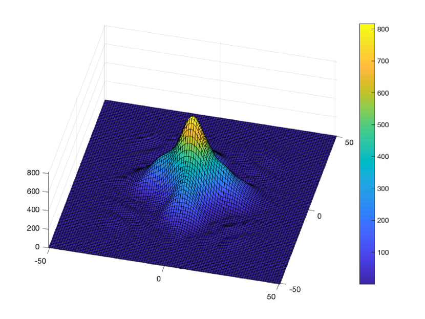
(b) Plot of $|\widehat{f}|$

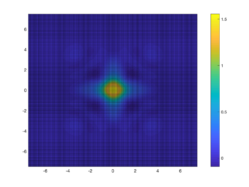
(c) Heat map of $|f|$

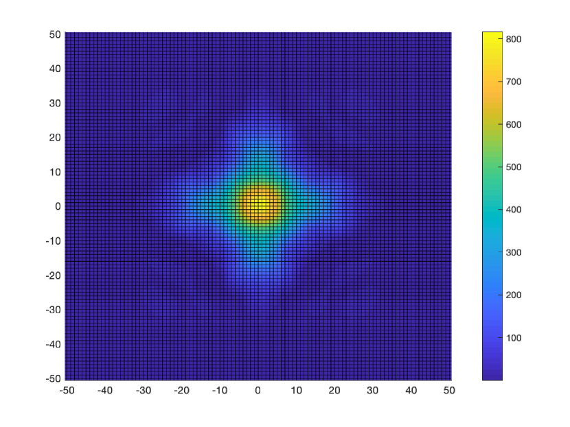
(d) Heat map of $|\widehat{f}|$

Figure 1. Various views of an optimizer $f$ for (A.1).

References

- [1] H. Bahouri, and P. Gérard, High frequency approximation of solutions to critical nonlinear wave equations, Amer. J. Math. 121 (1999), 131-175.
- [2] J. Bourgain. Refinements of Strichartz inequality and applications to 2D-NLS with critical nonlinearity, International Mathematics Research Notices, 8 (1998), 253-283.
- [3] E. Carneiro, L. Oliviera and M. Sousa. Gaussians never extremize Strichartz inequalities for hyperbolic paraboloids, preprint (2019).
- [4] T. Cazenave. Semilinear Schrödinger Equations, Courant Lecture Notes in Mathematics, 10, AMS Publishing, Providence (2003).
- [5] H. Chihara. Smoothing effects of dispersive pseudodifferential equations, Comm. Partial Differential Equations, 27, No. 9-10 (2002), 1953-2005.
- [6] B. Dodson, Global well-posedness and scattering for the defocusing, -critical, nonlinear Schrödinger equation when , Duke Math J., 165, No. 10 (2016), 3435-3516.
- [7] B. Dodson, Global well-posedness and scattering for the mass critical nonlinear Schrödinger equation with mass below the mass of the ground state, Adv. Math., 285 (2015), 1589-1618.
- [8] L. Fanelli and N. Visciglia. The lack of compactness in the Sobolev-Strichartz inequalities. J. Math. Pures et Appl, 99, No. 3, (2013), 309-320.
- [9] I. Gallagher. Profile decomposition for solutions of the Navier-Stokes equations, Bull. Soc. Math. France, 129 (2001), 285-316.
- [10] P. Gérard, Description du defaut de compacite de l’injection de Sobolev, ESAIM Control Optim. Calc. Var. 3 (1998), 213-233.
- [11] M. Ghidaglia and J.C. Saut, Nonexistence of Travelling Wave Solutions to Nonelliptic Nonlinear Schrodinger Equation, J. Nonlinear Sci. 6 (1996), 139–145.
- [12] D. Hundertmark and V. Zharnitsky, On sharp Strichartz inequalities in low dimensions, International Mathematics Research Notices 2006 (2006), 34080.
- [13] Dragos Iftimie, A Uniqueness Result for the Navier–Stokes Equations with Vanishing Vertical Viscosity, SIAM Journal on Mathematical Analysis 33, No. 6 (2002), 1483–1493.
- [14] C.E. Kenig and F. Merle, Global well-posedness, scattering and blow-up for the energy-critical, focusing, non-linear Schrödinger equation in the radial case, Inventiones Mathematicae 166, No. 3 (2006), 645-675.
- [15] C. E. Kenig, G. Ponce, C. Rolvung, and L. Vega. The general quasilinear ultrahyperbolic Schrödinger equation. Adv. Math. 196, No. 2 (2005), 402-433.
- [16] S. Keraani, On the Defect of Compactness for the Strichartz Estimates of the Schrödinger Equations, Journ. Diff. Eq. 175 (2001), 353-392.
- [17] R. Killip and M. Visan, Nonlinear Schrödinger Equations at Critical Regularity, Clay Summer School Lecture Notes, (2008).
- [18] S. Lee, Bilinear restriction estimates for surfaces with curvatures of different signs, Transactions of the American Mathematical Society 358, No. 8 (2006), 3511-3533.
- [19] F. Linares and G. Ponce, On the Davey-Stewartson systems, Annales de l’Institut Henri Poincare (C) Non Linear Analysis. 10, No. 5 (1993), 523-548.
- [20] P.-L. Lions. The concentration-compactness principle in the calculus of variations. The limit case, Part I, Revista Matemática Aberoamericana, 1, Issue 1 (1985), 145-201.
- [21] P.-L. Lions. The concentration-compactness principle in the calculus of variations. The limit case, Part II, Revista Matemática Aberoamericana, 1, Issue 2 (1985), 45-121.
- [22] P. Kevrekidis, A. Nahmod and C. Zeng. Radial standing and self-similar waves for the hyperbolic cubic NLS in 2D, Nonlinearity 24 (2011), No. 5, 1523-1538.
- [23] J.L. Marzuola, J. Metcalfe, D. Tataru. Quasilinear Schrödinger equation I: small data and quadratic interactions. Adv. Math., 231, No. 2 (2012), 1151-1172.
- [24] F. Merle and L. Vega. Compactness at blow - up time for solutions of the critical nonlinear Schrödinger equation in 2D. International Mathematics Research Notices, No. 8 (1998), 399-425.
- [25] A. Moyua, A. Vargas and L. Vega, Schrödinger maximal function and restriction properties of the Fourier transform, International Mathematics Research Notices, 1996, 793–815.
- [26] K.M. Rogers and A. Vargas. A refinement of the Strichartz inequality on the saddle and applications. J. Functional Anal., 241, No. 2 (2006), 212-231.
- [27] M. Ruzhansky and M. Sugimoto. Smoothing properties of evolution equations via canonical transforms and comparison principle, Proceedings of the London Mathematical Society 105, No. 2 (2012), 393-423.
- [28] Monique Sablé-Tougeron, Régularité microlocale pour des problemes aux limites non linéaires, Ann. Inst. Fourier 36, No. 1 (1986), 39–82.
- [29] S. Shao, Maximizers for the Strichartz and the Sobolev-Strichartz inequalities for the Schrödinger equation, Electronic Journal of Differential Equations (EJDE), (2009) Volume: 2009, page Paper No. 03, 13 p.
- [30] C. Sulem and P. Sulem. Nonlinear Schrödinger Equations, Springer (1999).
- [31] Terence Tao. A sharp bilinear restriction estimate for paraboloids. Geometric & Functional Analysis, 13, No. 6 (2003), 1359-1384.
- [32] N. Totz. A justification of the modulation approximation to the 3D full water wave problem. Communications in Mathematical Physics, 335, No. 1 (2015), 369-443.
- [33] N. Totz. Global Well-Posedness of 2D Non-Focusing Schrodinger Equations via Rigorous Modulation Approximation. J. Diff. Eq., 261, No. 4 (2016), 2251-2299.
- [34] N. Totz and S. Wu. A rigorous justification of the modulation approximation to the 2D full water wave problem. Comm. Math. Phys., 310, No. 3 (2012), 817-883.
- [35] A. Vargas. Restriction theorems for a surface with negative curvature. Math. Z., 249, (2005), 97-111.