Sales Forecast in E-commerce using
Convolutional Neural Network
Abstract
Sales forecast is an essential task in E-commerce and has a crucial impact on making informed business decisions. It can help us to manage the workforce, cash flow and resources such as optimizing the supply chain of manufacturers etc. Sales forecast is a challenging problem in that sales is affected by many factors including promotion activities, price changes, and user preferences etc. Traditional sales forecast techniques mainly rely on historical sales data to predict future sales and their accuracies are limited. Some more recent learning-based methods capture more information in the model to improve the forecast accuracy. However, these methods require case-by-case manual feature engineering for specific commercial scenarios, which is usually a difficult, time-consuming task and requires expert knowledge. To overcome the limitations of existing methods, we propose a novel approach in this paper to learn effective features automatically from the structured data using the Convolutional Neural Network (CNN). When fed with raw log data, our approach can automatically extract effective features from that and then forecast sales using those extracted features. We test our method on a large real-world dataset from CaiNiao.com and the experimental results validate the effectiveness of our method.
keywords:
Online markets; Sales forecast; Feature learning; CNN<ccs2012> <concept> <concept_id>10010147.10010257.10010258.10010259.10010264</concept_id> <concept_desc>Computing methodologies Supervised learning by regression</concept_desc> <concept_significance>300</concept_significance> </concept> <concept> <concept_id>10010147.10010257.10010293.10010294</concept_id> <concept_desc>Computing methodologies Neural networks</concept_desc> <concept_significance>500</concept_significance> </concept> <concept> <concept_id>10010405.10003550.10003555</concept_id> <concept_desc>Applied computing Online shopping</concept_desc> <concept_significance>500</concept_significance> </concept> </ccs2012>
[300]Computing methodologies Supervised learning by regression \ccsdesc[500]Computing methodologies Neural networks \ccsdesc[500]Applied computing Online shopping
1 Introduction
The dynamic and complex business environment in E-commerce brings great challenges to business decision making. Many intelligent technologies such as sales forecast are developed to overcome these challenges. Sales forecast is helpful for managing the workforce, cash flow and resources, such as optimizing the supply chain of manufacturers.
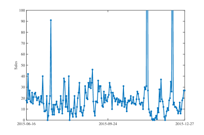
The value of sales forecast depends on its accuracy. Inaccurate forecasts may lead to stockout or overstock, hurting the decision efficiency in E-commerce. Traditional sales forecast techniques are based on time series analysis, which only take the historical sales data as the input. These methods can handle well commodities with stable or seasonal sales trends [9]. However, commodities in E-commerce are much more irregular in their sales trends (an example is shown in Figure 1) and the forecast accuracies achieved by these traditional methods are generally unacceptable [2].
Fortunately, a massive amount of data are available in E-commerce and it is possible to exploited these data to improve forecast accuracy. Besides the historical sales data, we can collect many other log data for online commodities over a long time period, such as page view (PV), page view from search (SPV), user view (UV), user view from search (SUV), selling price (PAY) and gross merchandise volume (GMV) etc. By using supervised learning methods such as regression models, these information can be integrated into the sales forecast model and better forecast accuracy can be achieved. The first step of the conventional machine learning methods is generally feature engineering, where effective features are extracted manually from the available data using domain knowledge [6]. The quality and quantity of features can greatly affect the accuracy of final forecast model. However, coming up with effective features is a difficult and time-consuming task. Moreover, these features are generally case-by-case extracted for specific commercial scenarios and models are difficult to be reused when data or requirements change. For instance, after more data are collected for online commodities, feature engineering should be done again to integrate the information contained in the new data into the sales forecast model.
Feature learning can obviate the need for manual feature engineering [3]. Through feature learning, effective features can be learned automatically from raw input data and then be used in specific machine learning tasks. Deep neural network is one of the most popular feature learning methods. It is inspired by the nervous system, where the nodes act as neurons and edges act as synapse. A neural network characterizes a function by the relationship between its input layer and output layer, which is parameterized by the weights associated with edges. Features are learned at the hidden layers and subsequently used for classification or regression at the output layer. There are many works using deep neural networks to learn features from the unstructured data, such as from image [11], audio [8], and text [4], etc.
In this paper, we propose a novel approach to learn effective features automatically from the structured data using the Convolutional Neural Network (CNN), which is one of the most popular deep neural network architectures. Firstly, we transform the log data of the commodity into a designed Data Frame. Then we apply Convolutional Neural Network on this Data Frame, where effective features will be extracted at the hidden layers and subsequently used for sales forecast at the output layer. Our approach takes the raw log data of commodities and it is easy to integrate new available data into the sales forecast model with few human intervention. What’s more, sample weight decay technique and transfer learning technique are used to improve the forecast accuracy further. We test our approach on a large real-world dataset from CaiNiao.com and the experimental results validate the effectiveness of our method.
The rest of our paper is organized as follows. We briefly review related works in section 2. We describe sales forecasting model in section 3 and the training of it in section 4. We show our experimental setup and results followed by discussion in section 5. Finally, we present our conclusions and plans to future research in section 6.
2 Related Work
Traditional sales forecast methods mainly exploit time series analysis techniques [9] [14]. Classical time series techniques include the autoregressive models (AR), integrated models (I), and moving average models (MA). These models predict future sales using a linear function of the historical sales data. More recent models, such as autoregressive moving average (ARMA) and autoregressive integrated moving average (ARIMA), are more general and can achieve better performance [24]. When used for sales forecast, these time series analysis models take the historical sales data as the input and are only suitable for commodities with stable or seasonal sales trends [2].
To better handle irregular sales patterns, some new methods attempt to exploit more information in sales forecast as an increasing amount of data are becoming available in E-commence. Kulkarni et al. [12] use online search data to forecast new product sales by using search term volume as a marketing metric. Ramanathan et al. [18] improve the forecast accuracy in promotional sales by incorporating product specific demand factors using multiple linear regression analysis. Yeo et al. [25] predict product sales by identifying customers purchase purpose from their browsing behavior. These methods are generally case-by-case developed for specific commercial scenarios and are limited in their applicability. They rely on specific domain knowledge to extract relevant features from the data, which is labor-intensive and exhibits their inability to extract and organize the discriminative information from the data.
Feature learning can obviate the need for manual feature engineering by learning effective features automatically from the raw input data [3]. Deep neural network is one of the most popular feature learning methods and its performances in many tasks have surpassed the conventional learning methods [11] [8] [4]. One particular family of deep neural networks named Convolutional Neural Network (CNN) was introduced by LeCun et al. [13] and rejuvenated in recent applications since the AlexNet [11] won the image classification challenge in ILSVRC2012 [19]. Then CNN experienced a strong surge from computer vision to speech recognition and natural language processing [23] [20] [21].
Deep neural networks can learn effective features at the hidden layers and then use these features for classification or regression at the output layer. Different from existing works, which learn features from the unstructured data (image, audio and text etc.), we intend to learn features automatically from the structured data using Convolutional Neural Network. That is learning effective features automatically from log data of commodities for sales forecast.
3 Sales Forecast Model
3.1 Problem formulation
We here describe the problem in a formal way. Given a commodity and certain geographic region in which the commodity sales are accumulated, we intend to forecast its total sales in this region over the time period , by using the commodity information and a sequence of related log data in time period . We use to denote the -dimensional item vector of commodity in region at time . The elements in are sales, page view (PV), page view from search (SPV), user view (UV), user view from search (SUV), selling price (PAY) and gross merchandise volume (GMV) etc. We denote the array of as the item matrix . The collection of intrinsic attributes of commodity are represented by vector , which includes category, brand and supplier etc.
Our goal is to build a mapping function to predict with and as the input:
| (1) |
where the parameter vector will be learned in the training process.
3.2 Forecasting with CNN
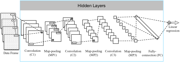
We forecast sales with function , which is a convolutional architecture as shown in Figure 2. In the following, we give a brief explanation of the main components in our CNN architecture.
3.2.1 Data Frame
Before using Convolutional Neural Network, we construct the Data Frame for each commodity based on its related log data and intrinsic attributes.
For each brand , category , and supplier , we calculate the brand vector , category vector , and supplier vector in region at time respectively:
| (2) |
| (3) |
| (4) |
We denote the array of , and as the brand matrix , the category matrix , and the supplier matrix respectively.
For each region , we calculate the region vector at time :
| (5) |
We denote the array of as the region matrix .
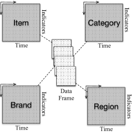
Finally, for each commodity in region , we construct its Data Frame as follow:
| (6) |
which is illustrated in Figure 3.
To forecast the sales of commodity in region , series operations including convolution, non-linear activation and pooling etc. are applied to the Data Frame .
3.2.2 Convolutional feature maps
Convolution can be seen as a special kind of linear operation, which aims to extract local patterns. In the context of sales forecast, we use the one-dimensional convolution to capture the shifting patterns in the time series of each input indicator individually.
More formally, the one-dimensional convolution is an operation between two vectors and . The vector is called as filter with size and the vector is a sequence with size . The specific operation is to take the dot product of the vector with each sub-sequence with length sliding along the whole sequence and obtain a new sequence , where:
| (7) |
In practice, we usually add a bias to the result of dot product. Thus we have:
| (8) |
According to the allowed range of index , there are two types of convolution: narrow and wide. The narrow convolution restricts in the range and yields a new sequence . The wide convolution restricts in the range and yields a new sequence . Note that when and , the values of are padded with zero. The benefits of wide convolution over the narrow one are discussed with details in [4]. Briefly speaking, unlike the narrow convolution where input values close to margins are seen fewer times, wide convolution gives equal attention to each value in the sentence and so is better at handling values at margins. More importantly, the wide convolution always produces a valid non-empty result even when . For these reasons, we use wide convolution in our model.
The indicator matrix in is not just a sequence of single indicator but a sequence of vectors including many indicators, where the dimension of each vector is . So when we apply the one-dimensional convolution on the indicator matrix , we need a filter bank consisting of filters with size and a bias bank consisting of baises. Each row of is convoluted with the corresponding row of and then the corresponding row of is added to the convolution result. After that, we obtain a matrix :
| (9) |
The values in filter bank and bias bank are parameters optimized during training. The filter size is a hyper-parameter of the model.
For each Data Frame , it has four indicator matrices, named item matrix , brand matrix , category matrix and region matrix . Therefore, we apply distinct convolutions to each indicator matrix respectively with filter bank and bias bank , and get four result matrices.
3.2.3 Activation function
To make the neural network capable of learning non-linear functions, a non-linear activation need to be applied to the output of preceding layer in an element-wise way. Then we obtain a new matrix :
| (10) |
Popular choices of include sigmod, tanh and relu (rectified linear defined as ). It has been shown that the choice of may affect the convergence rate and the quality of final solutions. In particular, Nair et al. [17] show that relu has significant edges because it overcomes some shortcomings of sigmoid and tanh. In practice, our experimental results are not very sensitive to the choice of activation and we choose relu due to its simplicity and computing efficiency.
In addition, we can see that the role played by the bias in (8) is to set an appropriate threshold for controlling units to be activated.
3.2.4 Pooling
After passing through the activation function, the output from convolutional layer is then passed to the pooling layer. Pooling layer will aggregate the information in the output of preceding layer. This operation aims to make the representation more robust and invariant to small translations in the input.
For a given vector , pooling with length aggregates each k-values in it into a single value one by one:
| (11) |
According to the way of aggregating the information, there are two types of pooling operations: average and max. Though both pooling methods have their own limitations, max-pooling is used more widely in practice.
When we apply pooling on the matrix , each row of is pooled respectively and we obtain a matrix :
| (12) |
3.2.5 Multiple feature maps
We have described how to apply a wide convolution, a non-linear activation and a pooling successively to an indicator matrix. After a group of those operations, we obtain the first order representation for learning to recognize specific shifting patterns in the input time series of indicators. To obtain higher order representations, we can use a deeper network by repeating these operations. Higher order representations are able to capture patterns in much longer range in the input time series of indicators.
Meanwhile, like the CNN in object recognition, we learn multi-aspect representations for each input indicator matrix. Let denote the -th order representation and we take the input Data Frame as the -th order representation. We compute representations in parallel at the -th order. Each representation is computed by two steps. Firstly, we apply convolution to each representation at the lower order with distinct filter bank and bias bank and then sum up the results. Secondly, non-linear activation and pooling are applied to the summation result. The whole process is as follow:
| (13) |
3.2.6 Fully connection
The last hidden layer of our CNN architecture is fully connection. Fully connection is a linear operation, which concentrates all representations at the highest order into a single vector. This vector can be seen as the features extracted from the original input.
More specifically, for the highest order representations (assume , we first flat them into a vector . Then we transform it with a dense matrix and apply non-linear activation:
| (14) |
where can been seen as the final extracted feature vector. The values in matrix are parameters optimized during training. The representation size is a hyper-parameter of the model.
3.2.7 Linear regression
After obtaining the feature vector , we use linear regression to forecast the final sales of commodity in region :
| (15) |
The values in vector are parameters optimized during training.
4 Training
We build a model for each region individually. For each region , our model is trained to minimize the mean squared error on an observed training set :
| (16) |
where is the real total sales of commodity in region over a time period , and is the corresponding forecasting result.
The parameters optimized in our neural network is :
| (17) |
namely the filter bank , bias bank , dense matrix and linear regression weight . Note that there are multiple filter banks and bias banks to be learned.
In the following, we present details in training our deep learning model.
4.1 Sample weight decay
By sliding the end point of the Data Frame, we can construct many training samples. However, each sample should have different importance: the closer to the target forecasting interval, the more important the training sample is. Let denote the start point of the target forecasting interval and denote the end point of the Data Frame of training sample . Obviously, holds, where is the length of forecasting interval. For each region , we assign a weight to each sample in the training set as follow:
| (18) |
where is a hyper-parameter.
Then for each region , instead of minimizing the mean squared error, we minimize the weighted mean squared error on the observed training set :
| (19) |
where is calculated as above.
4.2 Transfer learning
Transfer learning aims to transfer knowledge acquired in one problem onto another problem [15]. In the context of sales forecast, we can transfer learned patterns in one region onto another region.
We first train our neural network on the whole training set , which includes training samples in all regions:
| (20) |
After that, we replace with and continue training the specific model for each region respectively.
4.3 Regularization
Neural networks are capable of learning very complex functions and tend to easily overfit, especially on the training set with small and medium size. To alleviate the overfitting issue, we use a popular and efficient regularization technique named dropout [22]. Dropout is applied to the flatten vector in (14) before transforming it with the dense matrix . During the forward phase, a portion of units in are randomly dropped out by setting them to zero to prevent feature co-adaptation. The dropout rate is a hyper-parameters of the model. As suggested in [7], dropout is approximately equivalent to model averaging, which is an effective technique to generalize models in machine learning.
4.4 Hyper-parameters
The hyper-parameters in our deep learning model are set as follows: the size of filters and the length of pooling at the first order representation are ; the size of filters and the length of pooling at the second order representation are ; the size of filters and the length of pooling at the third order representation are . We intend to capture the patterns in the week level at the first order representation, the month and season level at the second and the third order representation respectively.
What’s more, the parameter of weight decay is ; the dimension of extracted feature vector is ; the dropout rate is ; there are 128 representations computed in parallel at each order representation, which means .
4.5 Optimization
To optimize our deep learning model, we use the Stochastic Gradient Descent (SGD) algorithm with shuffled mini-batches. The parameters are update through the back propagation framework (see [7] for its principle) with Adamax rule [10]. The batch size is set as 128 and the network is firstly pre-trained on the whole training set for 10 epochs and then trained on each training set for another 10 epochs. What’s more, normalization is usually helpful for the convergence of deep learning model, thus we normalize the input Data Frame by z-score method [26].
To exploit the parallelism of the operations for speeding up, we train our network on a GPU. A Python implementation using Keras111http://keras.io powered by Theano [1] can process 73k samples per minute on a single NVIDIA K2200 GPU.

5 Experiments
5.1 Dataset
We evaluate our deep learning model on a large dataset collected from CaiNiao.com222https://tianchi.aliyun.com/competition/
information.htm?raceId=231530,
which is the largest collaboration platform of logistics and supply chain in China.
The dataset is provide by Alibaba Group and it contains 1814892 records,
covering log data and attributes information of 1963 commodities in 5 regions ranging from 2014-10-10 to 2015-12-27.
There are log indicators, including sales, page view (PV), page view from search (SPV), user view (UV), user view from search (SUV), selling price (PAY) and gross merchandise volume (GMV) etc.
5.2 Setup
We here forecast the total sales of each commodity in each region over the time period [2015-12-21, 2015-12-27] by using the Data Frame in time period [2015-10-28, 2015-12-20]. That is to say the length of target interval is and the length of Data Frame is . After splitting all samples for each region into the training set and testing set, we have: the end points of Data Frame of training samples range from 2015-01-01 to 2015-12-13; the end point of Data Frame of testing samples is 2015-12-20. We compare our approach against several baselines and several different settings of our approach.
5.2.1 Baselines
| Region | 1 | 2 | 3 | 4 | 5 | Avrage |
|---|---|---|---|---|---|---|
| ARIMA | 104.37 | 96.68 | 190.50 | 397.08 | 87.18 | 175.16 |
| FE+GBRT | 97.36 | 83.90 | 187.06 | 329.81 | 82.21 | 156.07 |
| DNN | 97.50 | 73.55 | 181.67 | 347.50 | 82.17 | 156.48 |
| CNN | 96.98 | 72.22 | 151.96 | 326.39 | 80.91 | 145.69 |
| CNN+WD | 89.01 | 56.14 | 142.27 | 301.79 | 75.09 | 131.86 |
| CNN+WD+TL | 84.30 | 53.40 | 134.92 | 287.31 | 71.19 | 126.22 |
| Single-CNN | 101.92 | 75.70 | 159.48 | 343.54 | 85.04 | 153.22 |
ARIMA. ARIMA is a classical time series analysis technique. It takes the historical sales data as input and predicts the sales at the next time point directly.
FE+GBRT. We first extract 523 features manually, including UV of the previous day, average UV over previous three days, average UV over previous one week, average UV over previous one month, and whether there is a price reduction or not etc. After that, we use the Gradient Boosting Regression Tree (GBRT) to forecast the sales by taking those features as input.
DNN. DNN is the simplest neural network architecture, which puts multi-layers fully connection after the input. We first flat the Data Frame into a vector and then append 4 fully connection layers and a linear regression layer after the obtained input vector. The dimension of each fully connection is 1024 and a dropout with is apply to the output of last fully connection layer.
5.2.2 Different settings
CNN. The Convolution Neural Network architecture described in the section 3.2 is the foundation of our sales forecast model.
CNN+WD. To improve the accuracy of sales forecast, we assign weights to training samples according to the equation (18), and then train the CNN model to minimize the weighted mean squared error.
CNN+WD+TL. To improve the accuracy of sales forecast further, we intend to transfer the patterns learned from all training samples in onto each distinct region , which is described with details in section 4.2.
Single-CNN. We train an unified model using all training samples in and forecast sales for each region respectively. Note that there is no sample weight decay technique and transfer learning technique.
All results reported in the following sections is on the testing set and the metric we used to measure the performance is the mean squared error (MSE).
5.3 Result
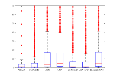
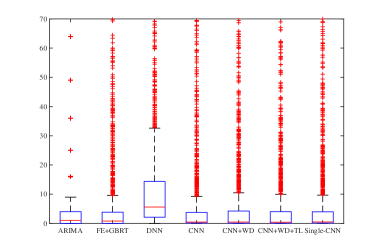
The detailed experimental results are presented in Figure 4 and the summary of those results is shown in Table 1.
The classical machine learning method (FE+GBRT) considers more information than the time series analysis method (ARIMA) and consequently achieves better performance. The simplest deep neural network architecture (DNN) extracts features automatically. Sometimes it even obtains more useful feature representation than feature engineering done by humans, which is shown in the experiment that DNN beats FE+GBRT in some situations.
The Convolution Neural Network architecture can make full use of the inherent structure in the raw data to extract more effective features and achieves a significant performance improvement. The sample weight decay technique and the transfer learning technique are highly effective. They further improve the performance and the final results are very competitive. Moreover, as we can see from the Figure 4, the forecast results from these two methods are more robust. It is interesting to explore whether it is possible to train one model for forecasting sales in all regions. So we train an unified model using all training samples in and forecast sales for each region respectively. The results are promising but less competitive than using individual models.
5.4 Discussion
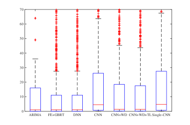
5.4.1 The length of target forecasting interval
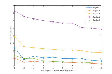
Figure 5 helps us to analyze the relationship between the length of target forecasting interval and the difficulty of forecasting. We can see that the longer the target forecasting interval, the easier the sales forecasting is. The main reason is that the total sales over a long target forecasting interval is more stable than that over a short forecasting interval. However, short forecasting interval allows more flexible business decision. So there is a typical tradeoff between the practical flexibility and the forecast accuracy in real-world applications.
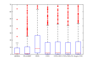
5.4.2 The length of Data Frame
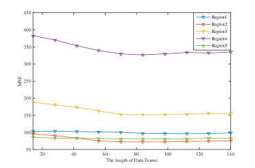
The length of Data Frame is a crucial hyper-parameter in our model. It represents how much historical data we used as the input of our model. As can be seen from Figure 6, if the Data Frame is too short the information contained in it is insufficient. On the other hand, long Data Frame may contain too much useless information, which confuses the learning machines. What’s more, longer Data Frame means more resources consumption in computing.
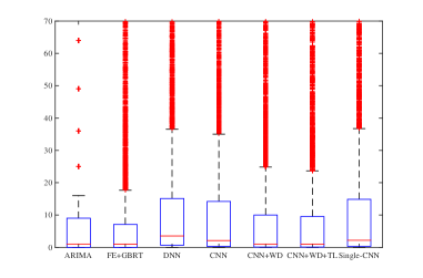
5.4.3 The intensity of weight decay
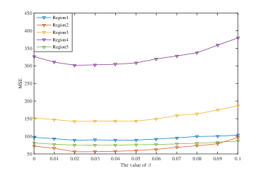
The value of in equation (18) controls the importance of training samples according to its closeness to the target forecasting interval. A large will make the model bias toward the closer training samples. As can be seen from Figure 7, achieves a good tradeoff between extracting long-term patterns and extracting shot-term patterns in log data for sales forecast.
6 Conclusions
In this paper, we present a novel approach to learn effective features automatically from the structured data using CNN. It can obviate the need for manual feature engineering, which is usually difficult, time-consuming and requires expert knowledge. We use the proposed approach to forecast sales by taking the raw log data and attributes information of commodities as the input. Firstly, we transform the log data and attributes information of commodities, which is in the structured type, into a designed Data Frame. Then we apply Convolutional Neural Network on the Data Frame, where effective features will be extracted at the hidden layers and subsequently used for sales forecast. We test our approach on a real-world dataset from CaiNiao.com and it demonstrates strong performance. What’s more, sample weight decay technique and transfer learning technique are used to improve the forecasting accuracy further, which have been proved to be highly effective in the experiments.
There are several interesting problems to be investigated in our further works: (1) Is it possible to find the most important indicators for sales forecast from the raw log data by deep neural networks; (2) It will be very appealing to find an unified framework for extracting features automatically from all types of data.
7 Acknowledgments
We would like to thank Alibaba Group for providing the valuable datasets.
References
- [1] F. Bastien, P. Lamblin, R. Pascanu, J. Bergstra, I. J. Goodfellow, A. Bergeron, N. Bouchard, and Y. Bengio. Theano: new features and speed improvements. Deep Learning and Unsupervised Feature Learning NIPS 2012 Workshop, 2012.
- [2] S. Beheshti-Kashi, H. R. Karimi, K.-D. Thoben, M. Lütjen, and M. Teucke. A survey on retail sales forecasting and prediction in fashion markets. Systems Science & Control Engineering, 3(1):154–161, 2015.
- [3] Y. Bengio, A. Courville, and P. Vincent. Representation learning: A review and new perspectives. IEEE transactions on pattern analysis and machine intelligence, 35(8):1798–1828, 2013.
- [4] P. Blunsom, E. Grefenstette, N. Kalchbrenner, et al. A convolutional neural network for modelling sentences. In Proceedings of the 52nd Annual Meeting of the Association for Computational Linguistics. Proceedings of the 52nd Annual Meeting of the Association for Computational Linguistics, 2014.
- [5] T. Chen and C. Guestrin. Xgboost: A scalable tree boosting system. arXiv preprint arXiv:1603.02754, 2016.
- [6] P. Domingos. A few useful things to know about machine learning. Communications of the ACM, 55(10):78–87, 2012.
- [7] I. Goodfellow, Y. Bengio, and A. Courville. Deep learning. Book in preparation for MIT Press, 2016.
- [8] A. Graves, A.-r. Mohamed, and G. Hinton. Speech recognition with deep recurrent neural networks. In 2013 IEEE international conference on acoustics, speech and signal processing, pages 6645–6649. IEEE, 2013.
- [9] G. Keller and N. Gaciu. Managerial statistics. South-Western Cengage Learning, 2012.
- [10] D. Kingma and J. Ba. Adam: A method for stochastic optimization. arXiv preprint arXiv:1412.6980, 2014.
- [11] A. Krizhevsky, I. Sutskever, and G. E. Hinton. Imagenet classification with deep convolutional neural networks. In Advances in neural information processing systems, pages 1097–1105, 2012.
- [12] G. Kulkarni, P. Kannan, and W. Moe. Using online search data to forecast new product sales. Decision Support Systems, 52(3):604–611, 2012.
- [13] Y. LeCun, L. Bottou, Y. Bengio, and P. Haffner. Gradient-based learning applied to document recognition. Proceedings of the IEEE, 86(11):2278–2324, 1998.
- [14] W.-I. Lee, B.-Y. Shih, and C.-Y. Chen. A hybrid artificial intelligence sales-forecasting system in the convenience store industry. Human Factors and Ergonomics in Manufacturing & Service Industries, 22(3):188–196, 2012.
- [15] J. Lu, V. Behbood, P. Hao, H. Zuo, S. Xue, and G. Zhang. Transfer learning using computational intelligence: A survey. Knowledge Based Systems, 80:14–23, 2015.
- [16] W. McKinney. pandas: a python data analysis library. see http://pandas. pydata. org, 2015.
- [17] V. Nair and G. E. Hinton. Rectified linear units improve restricted boltzmann machines. In Proceedings of the 27th International Conference on Machine Learning (ICML-10), pages 807–814, 2010.
- [18] U. Ramanathan. Supply chain collaboration for improved forecast accuracy of promotional sales. International Journal of Operations & Production Management, 32(6):676–695, 2012.
- [19] O. Russakovsky, J. Deng, H. Su, J. Krause, S. Satheesh, S. Ma, Z. Huang, A. Karpathy, A. Khosla, M. Bernstein, et al. Imagenet large scale visual recognition challenge. International Journal of Computer Vision, 115(3):211–252, 2015.
- [20] T. N. Sainath, B. Kingsbury, G. Saon, H. Soltau, A.-r. Mohamed, G. Dahl, and B. Ramabhadran. Deep convolutional neural networks for large-scale speech tasks. Neural Networks, 64:39–48, 2015.
- [21] A. Severyn and A. Moschitti. Learning to rank short text pairs with convolutional deep neural networks. In Proceedings of the 38th International ACM SIGIR Conference on Research and Development in Information Retrieval, pages 373–382. ACM, 2015.
- [22] N. Srivastava, G. E. Hinton, A. Krizhevsky, I. Sutskever, and R. Salakhutdinov. Dropout: a simple way to prevent neural networks from overfitting. Journal of Machine Learning Research, 15(1):1929–1958, 2014.
- [23] C. Szegedy, W. Liu, Y. Jia, P. Sermanet, S. Reed, D. Anguelov, D. Erhan, V. Vanhoucke, and A. Rabinovich. Going deeper with convolutions. In Proceedings of the IEEE Conference on Computer Vision and Pattern Recognition, pages 1–9, 2015.
- [24] W. W.-S. Wei. Time series analysis. Addison-Wesley publ Reading, 1994.
- [25] J. Yeo, S. Kim, E. Koh, S.-w. Hwang, and N. Lipka. Browsing2purchase: Online customer model for sales forecasting in an e-commerce site. In Proceedings of the 25th International Conference Companion on World Wide Web, pages 133–134. International World Wide Web Conferences Steering Committee, 2016.
- [26] D. Zill, W. S. Wright, and M. R. Cullen. Advanced engineering mathematics. Jones & Bartlett Learning, 2011.