Investigating the physical properties of transiting hot Jupiters with the 1.5-m Kuiper Telescope

Abstract

We present new photometric data of 11 hot Jupiter transiting exoplanets (CoRoT-12b, HAT-P-5b, HAT-P-12b, HAT-P-33b, HAT-P-37b, WASP-2b, WASP-24b, WASP-60b, WASP-80b, WASP-103b, XO-3b) in order to update their planetary parameters and to constrain information about their atmospheres. These observations of CoRoT-12b, HAT-P-37b and WASP-60b are the first follow-up data since their discovery. Additionally, the first near-UV transits of WASP-80b and WASP-103b are presented. We compare the results of our analysis with previous work to search for transit timing variations (TTVs) and a wavelength dependence in the transit depth. TTVs may be evidence of a third body in the system and variations in planetary radius with wavelength can help constrain the properties of the exoplanet’s atmosphere. For WASP-103b and XO-3b, we find a possible variation in the transit depths that may be evidence of scattering in their atmospheres. The B-band transit depth of HAT-P-37b is found to be smaller than its near-IR transit depth and such a variation may indicate TiO/VO absorption. These variations are detected from 2-4.6$\sigma$, so follow-up observations are needed to confirm these results. Additionally, a flat spectrum across optical wavelengths is found for 5 of the planets (HAT-P-5b, HAT-P-12b, WASP-2b, WASP-24b, WASP-80b), suggestive that clouds may be present in their atmospheres. We calculate a refined orbital period and ephemeris for all the targets, which will help with future observations. No TTVs are seen in our analysis with the exception of WASP-80b and follow-up observations are needed to confirm this possible detection.

1 Introduction

To date, over 3400 exoplanets have been discovered (NASA Exoplanet Archive; Akeson et al. 2013) and most of these planets have been found using the transit method (e.g. Charbonneau et al. 2000; Henry et al. 2000) in large-scale transit surveys such as Kepler (Borucki et al. 2010), K2 (Howell et al. 2014), WASP (Pollacco et al. 2006; Collier Cameron et al. 2007) and CoRoT (Baglin 2003; Moutou et al. 2013). Transiting exoplanet systems (TEPs) are of great interest because their radius can be directly measured in relation to their star with photometric observations (Charbonneau et al. 2000; Henry et al. 2000). With the addition of spectroscopic and radial velocity measurements, many physical properties of TEP systems (mass, radius, semi-major axis, gravity, temperature, eccentricity, orbital period) can be directly measured (e.g., Charbonneau et al. 2007). Additionally, multiple-band photometry of a TEP system can be used to constrain the composition of an exoplanet’s atmosphere (Seager & Sasselov 2000; Brown 2001; Hubbard et al. 2001; Charbonneau et al. 2002). The absorption properties of different species in a planetary atmosphere vary with wavelength, causing an observable variation in the planet’s radius. Photometric light curve analysis can also be used to search for transit timing variations (TTVs). TTVs can indicate additional bodies in a TEP system or an unstable orbit caused by tidal forces from the star (e.g., Miralda-Escudé 2002; Holman & Murray 2005; Holman et al. 2010).

In this work, we present new ground-based photometric data of 11 confirmed transiting hot Jupiter exoplanets. We describe and perform TEP modeling techniques (Section 2–3) to determine the orbital and physical parameters of each system, and compare our results with previous published results to confirm and improve the planetary parameters (Section 4–5). For each system, we combine our results with previous work to search for a variation in planetary radius with wavelength (Section 6), which could indicate Rayleigh scattering, the presence of an absorptive atmosphere, or clouds. Finally, we combine our mid-transit data with previous observations to recalculate each system’s orbital period and search for TTVs.

Table 1: Journal of observations

Planet	Date	Filter1	Cadence	Npts	OoT RMS2	Res RMS3	Seeing	ka	$\chi_{r}^{2}$ b
Name	(UT)		(s)		(mmag)	(mmag)	($\arcsec$)
CoRoT-12b	2013 February 15	R	60.39	265	6.06	4.99	1.96-4.06	4	1.32
HAT-P-5b	2015 June 6	U	80.64	191	3.02	2.84	1.36-2.17	4	0.97
HAT-P-12b	2014 January 19	B	188.25	89	1.13	1.27	2.22-2.96	7	1.99
HAT-P-33b	2012 April 6	R	24.29	706	3.65	4.15	1.01-2.68	4	7.84
HAT-P-37b	2015 July 1	B	115.51	128	2.37	2.88	0.98-2.45	4	1.10
HAT-P-37b	2015 July 1	R	115.51	129	2.33	2.30	0.98-2.45	4	1.33
WASP-2b	2014 June 14	B	59.31	230	2.41	2.28	1.43-2.68	7	3.55
WASP-24b	2012 March 23	R	24.95	531	2.41	2.55	1.03-2.12	7	4.06
WASP-24b	2012 April 6	R	26.77	434	5.14	5.73	1.01-2.72	6	2.04
WASP-60b	2012 December 1	B	20.46	751	5.30	4.65	0.83-6.82	4	1.21
WASP-80b	2014 June 16	U	93.50	160	7.76	7.20	1.54-2.92	7	1.15
WASP-103b	2015 June 3	U	65.05	363	3.66	3.62	1.37-2.56	6	1.29
XO-3b	2012 November 30	B	40.63	418	2.04	2.20	1.44-2.23	4	1.96

2 Observations and Data Reduction

All the observations were performed at the University of Arizona’s Steward Observatory 1.55-m Kuiper Telescope on Mt. Bigelow near Tucson, Arizona. The Mont4k CCD has a field of view of 9.7’$\times$9.7’ and contains a 4096$\times$4096 pixel sensor. The CCD is binned 3$\times$3 to achieve a resolution of 0.43$\arcsec$/pixel and binning reduces the read-out time to $\sim$10 s. Our observations were taken with the Bessell U (303–417 nm), Harris B (360–500 nm), and Harris R (550–900 nm) photometric band filters. To ensure accurate timing in these observations, the clocks were synchronized with a GPS every few seconds. In all the data sets, the average shift in the centroid of our targets is less than 0.6 pixels (0.26$\arcsec$) due to excellent autoguiding (the maximum is 3.4 pixels). This telescope has been used extensively in exoplanet transit studies (Dittmann et al. 2009b, a, 2010, 2012; Scuderi et al. 2010; Turner et al. 2013; Teske et al. 2013; Pearson et al. 2014; Biddle et al. 2014; Zellem et al. 2015; Turner et al. 2016b). A summary of all our observations are displayed in Table 1.

To reduce the data and create the light curves we use the reduction pipeline ExoDRPL (Pearson et al., 2014). Each of our images are bias-subtracted and flat-fielded with 10 biases and flats. To produce the light curve for each observation we perform aperture photometry (using phot in the IRAF DAOPHOT package) by measuring the flux from our target star as well as the flux from 8 different reference stars with 110 different circular aperture radii. The aperture radii sizes we explore are different for every observation due to changes in seeing conditions. For the analysis, a constant sky annulus for every night of observation of each target is chosen (a different sky annulus is used depending on the seeing and the crowdedness of the target field) to measure the brightness of the sky during the observations. We reduce the risk of contamination by making sure no stray light from the target star or other nearby stars falls in the chosen aperture. A synthetic reference light curve is produced by averaging the light curves from our reference stars. The final light curve of each date is normalized by dividing by this synthetic light curve to correct for any systematic differences from atmospheric variations (i.e. airmass) throughout the night. Every combination of reference stars and aperture radii are considered and we systematically choose the best aperture and reference stars by minimizing the scatter in the Out-of-Transit (OoT) data points. The 1$\sigma$ error bars on the data points include the readout noise, flat-fielding errors, and Poisson noise. The final light curves are presented in Figs. 1–3. The data points of all our transits are available in electronic form (see Table 2). For all the transits, the OoT baselines have a photometric root-mean-squared (RMS) value between 1.13 and 7.76 millimagnitude (mmag).

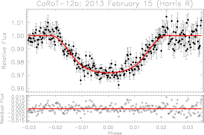
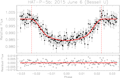
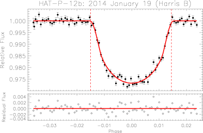
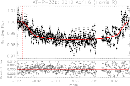
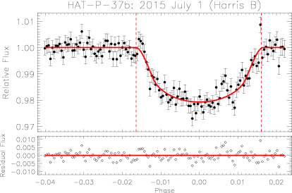
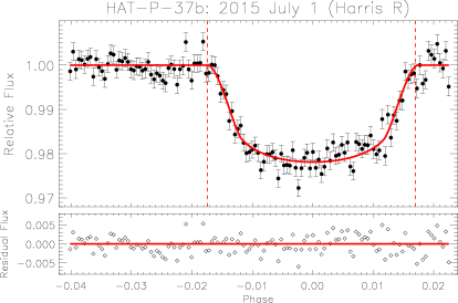
Figure 1: Light curves of CoRoT-12b, HAT-P-5b, HAT-P-12b, HAT-P-33b, and HAT-P-37b. The 1$\sigma$ error bars include the readout noise, the Poisson noise, and the flat-fielding error. The best-fitting models obtained from the EXOplanet MOdeling Package (EXOMOP) are shown as a solid red line. The model predicted ingress and egress points from EXOMOP are shown as dashed red vertical lines. The residuals (Light Curve - EXOMOP Model) are shown in the second panel. See Table 1 for the cadence, Out-of-Transit root-mean-squared (RMS) flux, and residual RMS flux for each light curve. The data points for all the transits are available in electronic form (see Table 2).

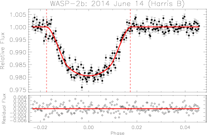
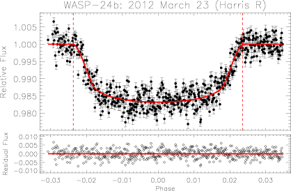
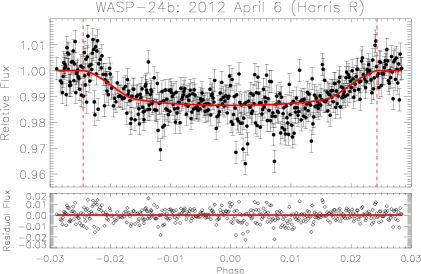
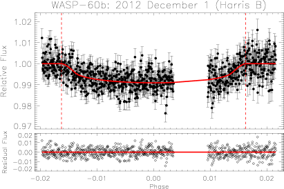
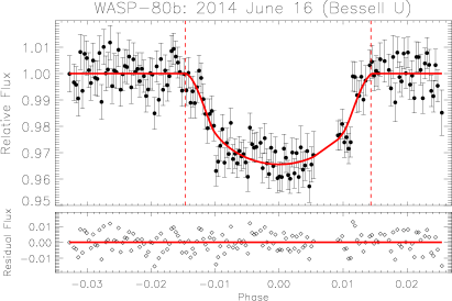
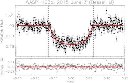
Figure 2: Light curves of WASP-2b, WASP-24b, WASP-60b, WASP-80b, and WASP-103b. Other comments are the same as Fig. 1.

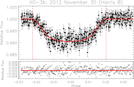
Figure 3: Light curve of XO-3b. Other comments are the same as Fig. 1.

Table 2: Photometry of all our light curves¹

Planet Name	Filter	Time (BJDTDB)	Relative flux	Error bars	CCD X-Pos	CCD Y-Pos	Median Airmass
CoRoT-12b	Harris-R	2456338.584736	0.99648	0.003327	529.411	635.689	1.513072
CoRoT-12b	Harris-R	2456338.585434	0.998034	0.003213	527.611	634.955	1.507972
CoRoT-12b	Harris-R	2456338.586133	0.998494	0.003108	528.101	634.46	1.502944
CoRoT-12b	Harris-R	2456338.586831	0.99549	0.003094	528.858	634.639	1.497979

3 Light Curve Analysis

To find the best-fit to the light curves we use the EXOplanet MOdeling Package (EXOMOP; Pearson et al. 2014; Turner et al. 2016b), which utilizes the analytic equations of Mandel & Agol (2002) to generate a model transit. For a complete description of EXOMOP see Pearson et al. (2014) and Turner et al. (2016b). The $\chi^{2}$-fitting statistic for the model light curve used in EXOMOP is:

$$\chi^{2}=\sum_{i=1}^{N_{pts}}\left[\frac{f_{i}(\mbox{obs})-f_{i}(\mbox{model})}{\sigma_{i}(\mbox{obs})}\right]^{2}$$ (1)

where $N_{pts}$ is the total number of data points (Table 1), $f_{i}(\mbox{obs})$ is the observed flux at time $i$, $\sigma_{i}(\mbox{obs})$ is the error in the observed flux, and $f_{i}(\mbox{model})$ is the calculated model flux.

EXOMOP uses the following procedure to find a best-fit to the data. A Levenberg-Marquardt (LM) non-linear least squares minimization (MPFIT; Markwardt 2009; Press et al. 1992) is performed on the data and a bootstrap Monte Carlo technique (Press et al. 1992) is used to calculate robust errors of the LM fitted parameters. Additionally, a Differential Evolution Markov Chain Monte Carlo (DE-MCMC; Braak 2006; Eastman et al. 2013) analysis is used to model the data. The fitted parameters that have the highest error bars from either the LM or DE-MCMC best-fitting model are used in the analysis. In every case both models find results within 1$\sigma$ of each other. Additionally, EXOMOP uses the residual permutation (rosary bead; Southworth 2008), time-averaging (Pont et al. 2006), and wavelet (Carter & Winn 2009) methods to assess the importance of red noise in both fitting methods. Not accounting for red noise in the data underestimates the fitted parameters (Pont et al. 2006; Carter & Winn 2009). In order to be conservative, the red noise method that produces the largest errors is used to inflate the errors in the fitted parameters. Finally, in order to compensate for underestimated observational errors we multiply the error bars of the fitted parameters by $\sqrt{\chi^{2}_{r}}$ when the reduced chi-squared ($\chi^{2}_{r}$) of the data (Table 1) is greater than unity (e.g. Bruntt et al. 2006; Southworth et al. 2007a; Southworth et al. 2007b; Southworth 2008; Barnes et al. 2013; Turner et al. 2016b).

EXOMOP uses the Bayesian Information Criterion (BIC; Schwarz 1978) to assess over-fitting of the data. The BIC is defined as

$$BIC=\chi^{2}+k\ln{(N_{pts})},$$ (2)

where $\chi^{2}$ is calculated for the best-fitting model (equation 1) and $k$ is the number of free parameters (Table 1) in the model fit [$f_{i}(\mbox{model})$]. The power of the BIC is the penalty for a higher number of fitted model parameters, making it a robust way to compare different best-fit models. The preferred model is the one that produces the lowest BIC value.

Each transit is modeled with EXOMOP using 10000 iterations for the LM model and 20 chains and 20⁶ links for the DE-MCMC model. The Gelman-Rubin statistic (Gelman & Rubin 1992) is used to ensure chain convergence (Ford 2006) in the MCMC model. During the analysis of each transit the mid-transit time ($T_{c}$), planet-to-star radius ($R_{p}/R_{*}$), scaled semi-major axis ($a/R_{*}$), and inclination ($i$) are set as free parameters. The previously published values for $a/R_{*}$, $i$, and $a/R_{*}$ are used as priors for the LM model (Table 3). The results of the LM fit are used as the prior for the DE-MCMC. The eccentricity ($e$), argument of periastron ($\omega$), and period ($P_{p}$) of each of the planets are fixed (see Table 3 for their values) in the analysis because these parameters have minimal effect on the overall shape of the light curve. The linear and quadratic limb darkening coefficients in each filter are taken from Claret & Bloemen (2011) and interpolated to the stellar parameters of the host stars (see Table 4) using the EXOFAST applet(Eastman et al., 2013). In addition, a linear or quadratic least squares fit is modeled to the OoT baseline simultaneously with the Mandel & Agol (2002) model. The BIC is used to determine whether to include any baseline fit in the best-fit model and the baseline with the lowest BIC value is always chosen.

The light curve parameters obtained from the EXOMOP analysis and the derived transit durations are summarized in Table 5. The modeled light curves can be found in Figs. 1–3 and the physical parameters for our targets are derived as outlined in Section 4 (Tables 6–7). A thorough description of the modeling and results of each system can be found in Section 5.

Table 3: Parameters fixed for the light curve fitting using EXOMOP

Planet	Period ($P_{p}$)	a/$R_{\ast}^{a}$	Inclination ($i$)a	Eccentricity ($e$)	Omega ($\omega$)	Source
	(days)		(∘)		(∘)
CoRoT-12b	2.828042	7.7402	85.48	0.070	105	1
HAT-P-5b	2.788491	7.5	86.75	0	0	2
HAT-P-12b	3.213089	11.7371	89.915	0	0	3
HAT-P-33b	3.474474	6.56	87.2	0.148	96	4
HAT-P-37b	2.797436	9.32	86.9	0.058	164	5
WASP-2b	2.15221812	8.06	84.89	0	0	6
WASP-24b	2.341213	5.98	83.64	0	0	7
WASP-60b	4.3050011	10	87.9	0	0	8
WASP-80b	3.06785	12.989	89.92	0.07	0	9
WASP-103b	0.925542	2.978	86.3	0	0	10
XO-3b	3.191524	7.07	84.2	0.26	345.8	11

Table 4: Limb darkening coefficients for the light curve fitting using EXOMOP

Planet	Filter	Linear coefficient1	Quadratic coefficient1	T${}_{\textrm{eff}}$ [K]	[Fe/H]	$\log{g}$ [cgs]	Source
CoRoT-12b	R	0.39440901	0.26682249	5675	0.160	4.375	1
HAT-P-5b	U	0.75552025	0.093484300	5960	0.240	4.368	2
HAT-P-12b	B	0.93774724	-0.083432883	4650	-0.290	4.610	3
HAT-P-33b	R	0.27628872	0.32295169	6401	0.05	4.15	4
HAT-P-37b	B	0.72832760	0.097543998	5500	0.03	4.52	5
HAT-P-37b	R	0.41967640	0.25020840	5500	0.03	4.52	5
WASP-2b	B	0.82272126	0.018632333	5200	0.100	4.537	2
WASP-24b	R	0.31410756	0.30624587	6080	-0.002	4.26	6
WASP-60b	B	0.61455358	0.18477201	5900	-0.040	4.20	7
WASP-80b	U	0.82663825	-0.029831771	4150	-0.140	4.60	8
WASP-103b	U	0.65536932	0.17875591	6110	0.060	4.22	9
XO-3b	B	0.50449954	0.25897027	6429	-0.177	3.950	10

Table 5: Light curve parameters derived in this study using EXOMOP

Planet	CoRoT-12b	HAT-P-5b	HAT-P-12b	HAT-P-33b	HAT-P-37b
Date	2013 February 15	2015 June 6	2014 January 19	2012 April 6	2015 July 1
Filter1	R	U	B	R	B
$T_{c}$ (BJDTDB-2450000)	6338.67097$\pm 0.00074$	7180.82658$\pm 0.00076$	6677.97482$\pm 0.00047$	6024.71746$\pm 0.0012$	7205.91376$\pm 0.00054$
Rp/R∗	0.1645${}^{+0.0038}_{-0.0040}$	0.1225$\pm 0.0051$	0.1386${}^{+0.0013}_{-0.0014}$	0.1152$\pm 0.0017$	0.1253$\pm 0.0021$
$a/R_{*}$	6.59${}^{+0.31}_{-0.29}$	6.05$\pm 0.44$	11.86$\pm 0.57$	5.67$\pm 0.13$	10.82$\pm 0.91$
Inclination (∘)	83.54$\pm 0.71$	83.31$\pm 1.11$	90.98$\pm 1.09$	90.08$\pm 3.43$	89.99$1.83$
Duration (mins)	174.0$\pm 1.4$	184.1$\pm 1.9$	139.8$\pm 4.4$	270.45$\pm 0.48$	132.8 $\pm$ 2.7
Red noise (mmag)	0.0001	1.60	0.21	0.78	0.0001
OoT baseline function	None	None	Quadratic	None	None
Planet	HAT-P-37b	HAT-P-37b	WASP-2b	WASP-24b	WASP-24b
Date	2015 July 1	Weighted Average	2014 June 14	2012 March 23	2012 April 6
Filter1	R	—	B	R	R
$T_{c}$ (BJDTDB-2450000)	7205.91325$\pm 0.00056$	—	6823.83839$\pm 0.00055$	6010.8437$-0.0017$	6024.8910$\pm 0.0015$
Rp/R∗	0.1361$\pm 0.0028$	0.1291$\pm 0.0017$	0.1383$\pm$0.0049	0.1139$\pm$0.0015	0.1113$\pm 0.0043$
$a/R_{*}$	9.14$\pm 0.63$	9.68$\pm 0.52$	8.05$\pm{1.21}$	7.42$\pm 0.15$	6.06$\pm 0.73$
Inclination (∘)	86.73$\pm 0.93$	87.4$\pm 0.82$	84.86$\pm 1.61$	90.0$\pm 5.4$	83.95$\pm 2.74$
Duration (mins)	140.5 $\pm$ 2.7	136.6$\pm$1.9	108.4$\pm 1.4$	159.5$\pm 0.6$	165.0$\pm 0.6$
Red noise (mmag)	0.34	—	0.00	0.27	0.60
OoT baseline function	None	—	Quadratic	Quadratic	Linear
Planet	WASP-24b	WASP-60b	WASP-80b	WASP-103b	XO-3b
Date	Weighted Average	2012 December 1	2014 June 16	2015 June 3	2012 November 30
Filter1	R	B	U	U	B
$T_{c}$ (BJDTDB-2450000)	—	6263.6330$\pm 0.0012$	6824.88661$\pm 0.00091$	7177.8222${}^{+0.0015}_{-0.0009}$	6262.6566$\pm 0.0015$
Rp/R∗	0.1136$\pm 0.0014$	0.0852$\pm 0.0036$	0.1615$\pm 0.0033$	0.1181$\pm$0.0016	0.0968$\pm 0.0023$
$a/R_{*}$	7.36$\pm$0.15	9.49$\pm 1.81$	12.85$\pm 0.42$	2.90$\pm 0.05$	5.68$\pm 0.51$
Inclination (∘)	85.19$\pm 2.44$	87.48$\pm 2.83$	90.0$\pm 1.8$	90.00$\pm 0.18$	81.75$\pm 0.77$
Duration (mins)	162.1$\pm 0.4$	201.9$\pm 0.3$	126.7 $\pm 2.2$	167.6 $\pm 1.5$	185.4 $\pm 0.9$
Red noise (mmag)	—	0.00	0.01	0.001	0.001
OoT baseline function	—	None	Quadratic	Linear	None

4 Physical Properties of the Systems

We use the results of our light curve modeling with EXOMOP combined with other measurements in the literature to calculate the planetary mass (e.g. Winn 2010; Seager 2011), radius, density, surface gravity (e.g. Southworth et al. 2007a), modified equilibrium temperature (e.g. Southworth 2010), Safronov number (e.g. Safronov 1972; Southworth 2010), and atmospheric scale height (e.g. Seager 2011; de Wit & Seager 2013). An updated period and ephemeris is also calculated and is described in detail in Section 4.1. To calculate the physical parameters we use the values from the modeling ($P_{p}$, $R_{p}/R_{\ast}$, $i$, $a/R_{\ast}$) and for the orbital ($e$) and host star parameters (radial velocity amplitude, mass, radius, equilibrium temperature) we use the values found in the literature. When calculating the scale height, the mean molecular weight in the planet’s atmosphere was set to 2.3 assuming a H/He-dominated atmosphere (de Wit & Seager 2013). The physical parameters of all our systems can be found in Tables 6–7.

Table 6: Physical parameters derived in this study for CoRoT-12b, HAT-P-5b, HAT-P-12b,HAT-P-33b, HAT-P-37b, WASP-2b, WASP-24b, WASP-60b, and WASP-80b.

Planet	CoRoT-12b	HAT-P-5b	HAT-P-12b
Date	2013 February 15	2015 June 6	2014 January 19
Period (Days)	2.828051 $\pm 0.000080$	2.78847280 $\pm 0.00000039$	3.21305761 $\pm 0.00000020$
$T_{c}(0)$ (BJD-2450000)	4398.628 $\pm 0.055$	4241.77716 $\pm 0.00015$	4187.85623 $\pm 0.00013$
Mb (MJup)	0.922 $\pm$ 0.072	1.06 $\pm$ 0.12	0.211$\pm$0.012
Our Rb (RJup)	1.79 $\pm$ 0.15	1.36 $\pm$ 0.057	0.949$\pm$0.017
Reference Rb (RJup)	1.44 $\pm$ 0.13 (a)	1.26 $\pm$ 0.05 (b)	0.959$\pm$0.029 (c)
$\rho_{b}$ (cgs)	0.200 $\pm$ 0.054	0.531 $\pm$ 0.088	0.306$\pm$0.023
$\log{g_{b}}$ (cgs)	2.72 $\pm$ 0.12	2.946 $\pm$ 0.085	2.77$\pm$0.052
T${}^{{}^{\prime}}_{eq}$ (K)	1563 $\pm$ 22	1713 $\pm$ 29	954$\pm$12
$\Theta$	0.0327 $\pm$ 0.0054	0.0431 $\pm$ 0.0064	0.0235$\pm$0.0019
a (au)	0.0342 $\pm$ 0.0032	0.0320 $\pm$ 0.0023	0.0386$\pm$0.0019
H (km)	1521 $\pm$ 402	979 $\pm$ 193	822 $\pm$ 98
Planet	HAT-P-33b	HAT-P-37b	WASP-2b
Date	2012 April 6	2015 July 1	2014 June 14
Period (Days)	3.4744750$\pm$0.00000037	2.79744149 $\pm$0.00000083	2.15222114 $\pm$0.00000019
$T_{c}(0)$ (BJD-2450000)	5110.92726$\pm 0.00012$	5616.96710$\pm$ 0.00028	3991.515553 $\pm 0.000074$
Mb (MJup)	1.26$\pm$0.23	1.17 $\pm$ 0.10	0.880 $\pm$ 0.087
Our Rb (RJup)	1.99$\pm$0.32	1.16 $\pm$ 0.06	1.12 $\pm$ 0.13
Reference Rb (RJup)	1.827$\pm$0.290 (d)	1.178 $\pm$ 0.077 (e)	1.043 $\pm$ 0.033 (f)
$\rho_{b}$ (cgs)	0.20$\pm$0.10	0.93 $\pm$ 0.17	0.77 $\pm$ 0.28
$\log{g_{b}}$ (cgs)	2.83$\pm$0.21	3.369 $\pm$ 0.088	3.25 $\pm$ 0.18
T${}^{{}^{\prime}}_{eq}$ (K)	1901$\pm$26	1250 $\pm$ 22	1284 $\pm$ 20
$\Theta$	0.042 $\pm$ 0.013	0.085 $\pm$ 0.012	0.058 $\pm$ 0.016
a (au)	0.0468 $\pm$ 0.0075	0.0394 $\pm$ 0.0029	0.0312 $\pm$ 0.0056
H (km)	1408$\pm$679	270 $\pm$ 54	364 $\pm$ 155
Planet	WASP-24b	WASP-60b	WASP-80b
Date	Combined	2012 December 1	2014 June 16
Period (Days)	2.34121877 $\pm 0.00000030$	4.305022 $\pm 0.000021$	3.06785925 $\pm 0.00000047$
$T_{c}(0)$ (BJD-2450000)	4945.589444 $\pm 0.000090$	5747.0302$\pm 0.0022$	6125.418034$\pm 0.000052$
Mb (MJup)	1.032 $\pm$ 0.037	0.512$\pm$ 0.034	0.551$\pm$ 0.036
Our Rb (RJup)	1.27 $\pm$ 0.055	0.94$\pm$ 0.12	0.99$\pm$ 0.24
Reference Rb (RJup)	1.303 $\pm$ 0.047 (g)	0.86$\pm$ 0.12 (h)	0.999$\pm$ 0.031 (i)
$\rho_{b}$ (cgs)	0.628 $\pm$ 0.085	0.75$\pm$ 0.27	0.71$\pm$ 0.51
$\log{g_{b}}$ (cgs)	3.279 $\pm$ 0.057	3.11$\pm$ 0.22	3.22$\pm$ 0.29
T${}^{{}^{\prime}}_{eq}$ (K)	1583 $\pm$ 27	1354$\pm$ 23	817$\pm$ 20
$\Theta$	0.0566 $\pm$ 0.0043	0.051$\pm$ 0.013	0.072$\pm$ 0.025
a (au)	0.0392 $\pm$ 0.0018	0.050$\pm$ 0.011	0.0376 $\pm$ 0.0090
H (km)	421 $\pm$ 55	536 $\pm$ 274	248 $\pm$ 168

Table 7: Physical parameters derived in this study for WASP-103b and XO-3b

Planet	WASP-103b	XO-3b
Date	2015 June 3	2012 November 30
Period (days)	0.9255454 $\pm 0.0000010$	3.19153125 $\pm 0.00000053$
$T_{c}(0)$ (BJD-2450000)	6459.59948 $\pm 0.00041$	2997.72200 $\pm 0.00040$
Mb (MJup)	1.484 $\pm$ 0.082	13.07$\pm$ 0.66
Our Rb (RJup)	1.640 $\pm$ 0.066	1.403$\pm$ 0.093
Previous Rb (RJup)	1.528 $\pm$ 0.073 (a)	1.217$\pm$ 0.073 (b)
$\rho_{b}$ (cgs)	0.417 $\pm$ 0.055	5.87$\pm$ 1.20
$\log{g_{b}}$ (cgs)	3.114 $\pm$ 0.055	4.05$\pm$ 0.11
T${}^{{}^{\prime}}_{eq}$ (K)	2537 $\pm$ 42	2011$\pm$ 13
$\Theta$	0.0286 $\pm$ 0.0023	0.519$\pm$ 0.075
a (au)	0.09361 $\pm$ 0.00078	0.0393$\pm$ 0.0041
H (km)	986 $\pm$ 125	90 $\pm$ 22

4.1 Period Determination

By combining our mid-transit times found using EXOMOP with previously published mid-transit times, we can refine the orbital period of the targets. When necessary, the mid-transit times were transformed from HJD, which is based on UTC time, into BJD, which is based on Barycentric Dynamical Time (TDB), using the online converter by Eastman et al. (2010). A refined ephemeris for each target is found by performing a weighted linear least-squares analysis using the following equation:

$$T_{c}=T_{c}(0)+P_{p}\times{E},$$ (3)

where $T_{c}(0)$ is the mid-transit time at the discovery epoch measured in $BJD_{TDB}$, $P_{p}$ is the orbital period of the target and $E$ is the integer number of cycles after their discovery paper. See Tables 6-7 for an updated T_c and P_b for each system.

For every system, we also made observation minus calculation mid-transit time (O-C) plots in order to search for any TTVs due to other bodies in the system. We used the derived period and ephemeris found in Tables 6-7 and Equation 3 for the calculated mid-transit times. The O-C plots can be found in Figs 4–5. The transit timing analysis for all our targets can be found in Table 8 (the entire table can be found online). We do not observe any significant TTVs in our data with the exception of a 3.8$\sigma$ deviation for WASP-80b for our observed transit. Since the possible TTV is only one data point and may be caused by an unknown systematic error, more observations of WASP-80b are needed to confirm this result.

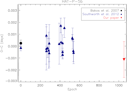
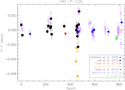
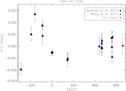
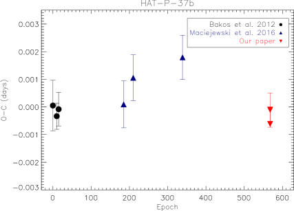
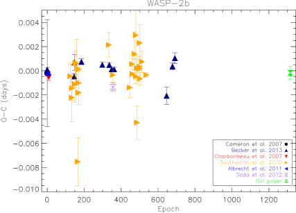
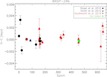
Figure 4: Observation minus calculation mid-transit time (O-C) plots of HAT-P-5b, HAT-P-12b, HAT-P-33b, WASP-2b, and WASP-24b from this paper and previous literature. We do not see any evidence for TTVs.

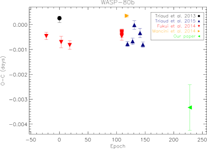
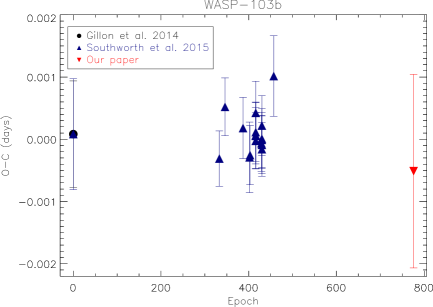
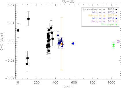
Figure 5: O-C plot of WASP-80b, XO-3b, and WASP-103b from this paper and previous literature. We do not see any TTVs with the exception of WASP-80b but there are large uncertainties in our measurement, so we recommend follow-up observations to verify this claim.

Table 8: Results of the transit timing analysis¹

Planet Name	$T_{c}$ ($BJD_{TDB}$)	$T_{c}$ error (d)	Epoch	O-C (d)	O-C error (d)	Source
CoRoT-12b	2456338.67097	0.00074	686	-0.0000012	0.055	This paper
CoRoT-12b	2454398.628	0.055	0	0.00000000046	0.078	Gillon et al. 2010

5 Individual Systems

5.1 CoRoT-12b

CoRoT-12b was discovered by the CoRoT satellite (Carone et al. 2012) and was confirmed by follow-up photometry and radial-velocity measurements (Gillon et al. 2010). CoRoT-12b is an inflated hot Jupiter with a low density that is well predicted by standard models (Fortney et al. 2007) for irradiated planets (Gillon et al. 2010).
We observed a transit of CoRoT-12b on 2013 February 15 with the Harris R filter (Fig. 1). We find a $R_{p}/R_{\ast}$ value 4.6$\sigma$ greater than the discovery value. Our derived physical parameters are in good agreement with Gillon et al. (2010). We find a planetary radius within 1.3$\sigma$ of the previously calculated value and a planetary mass within 1$\sigma$ (Tables 5 and 6).

5.2 HAT-P-5b

HAT-P-5b is a hot Jupiter discovered by the HATNet project that orbits a slightly metal-rich star (Bakos et al. 2007). Follow-up multi-color transit observations of HAT-P-5b by Southworth et al. (2012) confirmed the existence of the planet and searched for a variation in planetary radius with wavelength. A significantly larger radius was found in the U-band than expected from Rayleigh scattering alone, which the authors suggest may be due to an unknown systematic error.

We observed a transit of HAT-P-5b on 2015 June 6 with the Bessell U filter (Fig. 1). Our derived physical parameters are in agreement with previous literature (Tables 5 and 6). We derive a U-band radius consistent with a weighted average of radii taken from 350-733 nm within 1$\sigma$ (Table 9; Fig 6). The error on our U-band observation is too large to determine if the observation by Southworth et al. (2012) in the same band may have an unknown systematic error (as suggested by them). Our calculated period is in good agreement with the value found by Southworth et al. (2012) with a similar uncertainty.

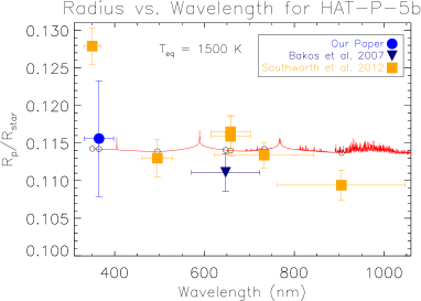
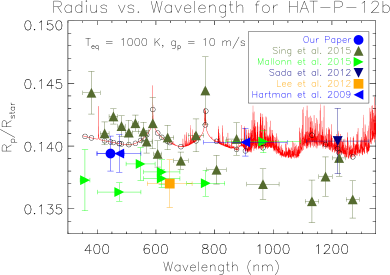
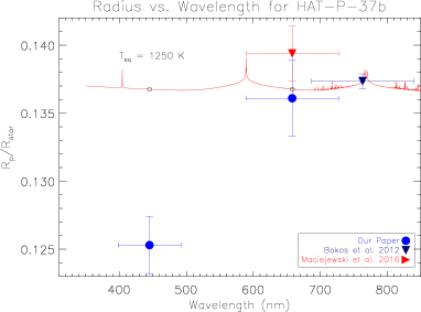
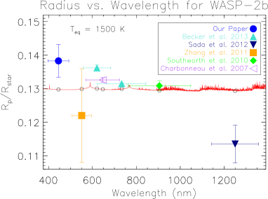
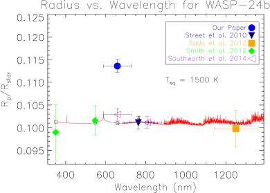
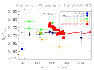
Figure 6: Plot of $R_{p}/R_{*}$ against wavelength for HAT-P-5b, HAT-P-12b, HAT-P-37b, WASP-2b, WASP-24b, and WASP-80b from this paper and previous literature. Our data are shown as blue circles. Over-plotted in red are atmospheric models by Fortney & Nettelmann (2010) for planets with a 1 $M_{Jup}$, $g_{p}=25m\ s^{-1}$ (unless specified on plot), $T_{eq}$ (specified on plot), and a base radius of 1.25 $R_{Jup}$ at 10 bar. We find that HAT-P-5b, HAT-P-12b, WASP-2b, and WASP-80b have flat spectra that could indicate the presence of clouds. The transit depth variation of HAT-P-37b could be due to absorption of TiO/VO (Evans et al. 2016).

Table 9: $R_{p}$/$R_{*}$ and effective central wavelength $\lambda_{\textrm{eff}}$ from this paper and previous literature for all targets¹.

Planet	Filter	Wavelength (nm)	Rp/$R_{*}$	Source
CoRoT-12b	Harris R	658	0.1645$\pm$0.0040	This Paper
CoRoT-12b	Clear	400-900	0.1321$\pm$0.0011	Gillon et al. 2010

5.3 HAT-P-12b

HAT-P-12b is a low density, sub-Saturn mass planet discovered by the HAT survey (Hartman et al. 2009). Multiple photometric studies have further refined the system’s parameters and searched for TTVs (Sada et al. 2012; Sokov et al. 2012; Lee et al. 2012; Line et al. 2013; Mallonn et al. 2015b; Sing et al. 2016; Sada & Ramón-Fox 2016). Sing et al. (2016) find a strong optical scattering slope from blue to near-IR wavelengths using Hubble Space Telescope and Spitzer Space Telescope transmission spectrum data.

We observed a transit of HAT-P-12b on 2014 January 19 using the Harris B filter (Fig. 1). We derive an optical R_p/R_∗ within 1$\sigma$ of previously derived radii at optical wavelengths (Table 9; Fig 6). These results are consistent with the planet having high clouds in its atmosphere (e.g. Seager & Sasselov 2000; Kreidberg et al. 2014) and the finding by Line et al. (2013) that HAT-P-12b has a cloudy atmosphere. We also find a period similar to Mallonn et al. (2015b).

5.4 HAT-P-33b

HAT-P-33b is an inflated hot Jupiter orbiting a high-jitter star (Hartman et al., 2011). The high-jitter is believed to be caused by convective inhomogeneities in the host star (Saar et al. 1998; Hartman et al. 2011). The planetary radius and mass, which both depend on eccentricity, and the stellar parameters are not well constrained due to the large jitter ( 20  m  s^-1). HAT-P-33b’s radius is either 1.7 or 1.8 $R_{Jup}$ assuming a circular or eccentric orbit, respectively. The first follow-up observations by the Transiting Exoplanet Monitoring Project (TEMP) of HAT-P-33b confirmed the discovery parameters and detected no signs of TTVs (Wang et al. 2017).

We observed one transit of HAT-P-33b on 2012 April 6 with the Harris R filter (Fig. 1). We find a R-band R_p/R_∗ value that is larger by 3.4$\sigma$ from the discovery R_p/R_∗ (Table 9). Follow-up observations are need to determine the cause of this discrepancy.

5.5 HAT-P-37b

HAT-P-37b was identified by the HATNet survey and was confirmed by high-resolution spectroscopy and further photometric observations (Bakos et al. 2012). HAT-P-37b is a hot Jupiter with a planetary mass of 1.169$\pm$0.103 $M_{Jup}$, a radius of 1.178$\pm$0.077 $R_{Jup}$, and a period of 2.797436$\pm$0.000007 $d$. Additional follow-up observations by Maciejewski et al. (2016) confirmed these planetary parameters.

We obtained two transits of HAT-P-37b on 2015 July 1 with the Harris B and R filters (Fig. 1). We derive an R_p/R_∗ for each filter that differ by 1.7$\sigma$, with a larger radius in the R band (Table 9; Fig 6). The B-band R_p/R_∗ is smaller by 2.85$\sigma$ from the near-IR R_p/R_∗ (Table 9; Bakos et al. 2012). Our derived R-band R_p/R_∗ value agrees within 1$\sigma$ of the Sloan i band value obtained by Bakos et al. (2012). Near-UV observations are needed to determine if the slope between the B and R filters is real or an unknown systematic in the data. Our other derived physical parameters agree with previous literature to within 1$\sigma$ (Tables 5 and 6). We also calculate a refined period with a factor of 6 decrease in error.

5.6 WASP-2b

WASP-2b is a short-period hot Jupiter discovered by the WASP survey and confirmed by radial-velocity measurements taken with the SOPHIE spectrograph (Collier Cameron et al. 2007). Extensive photometry and radial velocity measurements have been performed on WASP-2b, further refining its system parameters (Charbonneau et al. 2007; Daemgen et al. 2009; Southworth et al. 2010; Triaud et al. 2010; Albrecht et al. 2011; Zhang et al. 2011; Husnoo et al. 2012; Sada et al. 2012; Becker et al. 2013).

We observed WASP-2b on 2014 June 14 with the Harris B filter (Fig. 2). Our derived physical parameters and transit depth agree with previous literature to within 1$\sigma$ and we calculate a period with a factor of 2 decrease in error (Tables 5 and 6).

5.7 WASP-24b

WASP-24b is a hot Jupiter detected by WASP and confirmed by radial velocity measurements and additional photometric observations (Street et al. 2010). Further photometric studies calculated improved system parameters (Southworth et al. 2014) and radial velocity measurements were used to determine that the planet exhibits a symmetrical Rossiter-McLaughlin effect, indicating a prograde, well-aligned orbit (Simpson et al. 2011).

Our observations of WASP-24b took place on 2012 March 23 and 2012 April 6 (Fig. 2). We obtained two transits with the Harris R filter and each transit was modeled separately. The R_p/R_∗ of both dates overlap each other within 1$\sigma$. We then found the weighted average of the light curve parameters before deriving the physical parameters. Our weighted average R_p/R_∗ disagrees with previous R-band observations (Southworth et al. 2014) by 4$\sigma$ (Table 9; Fig 6). The cause of this difference is unknown but future observations can put better constraints on transit depth and solve this discrepancy. Our other derived parameters generally agree with previous results except for our planetary radius and equilibrium temperature, which differ from Southworth et al. (2014) by 1.4$\sigma$ and 1.9$\sigma$, respectively (Tables 5 and 6). We calculate a new period with a factor of 2.6 decrease in error (Table 6).

5.8 WASP-60b

WASP-60b was identified by WASP-North and was confirmed by radial-velocity measurements and follow-up photometry (Hébrard et al. 2013). WASP-60b is an unexpectedly compact planet orbiting a metal-poor star.

We observed a transit of WASP-60b with the Harris B filter on 2012 December 1 (Fig. 2). This observation is the first follow-up light curve of WASP-60b. During observations, the automatic guider briefly failed, resulting in a hole in the transit light curve. Despite this, we are able to derive parameters that agree with previous literature to within 1$\sigma$ (Tables 5 and 6). We find a B-band $R_{p}/R_{\ast}$ value 1.3$\sigma$ greater than the discovery $R_{p}/R_{\ast}$.

5.9 WASP-80b

WASP-80b is a warm Saturn/hot Jupiter ($M_{p}=0.55\pm 0.04M_{jup}$) with one of the largest transit depths (0.17126$\pm$0.00031) discovered so far (Triaud et al. 2013). Multiple photometric studies have been done at various wavelengths to refine WASP-80b’s planetary parameters (Fukui et al. 2014; Mancini et al. 2014; Triaud et al. 2015; Salz et al. 2015; Sedaghati et al. 2017). The planet has a transmission spectrum consistent with thick clouds and atmospheric haze (Fukui et al. 2014).

We observed WASP-80b on 2014 June 16 with the Bessell U filter, obtaining one transit (Fig. 2). Inclement weather conditions caused our guider to briefly fail, resulting in a hole in the transit light curve. We derive physical parameters that closely agree with previous literature and also calculate a slightly a refined period with a factor of 2 decrease in error (Tables 5 and 6). Our observations possibly detect a TTV compared to previous work by 3.7$\sigma$ (Section 4.1), however, further observations of WASP-80b are needed in order to confirm this result.

5.10 WASP-103b

WASP-103b is a hot Jupiter detected by the WASP survey with a mass of 1.49$\pm$0.09 $M_{jup}$, short period planet ($P_{p}=0.925542\pm 0.000019\ \rm{d}$), and has an orbital radius only 20% larger than its Roche radius (Gillon et al. 2014). It was found that there is a faint, cool, and nearby (with a sky-projected separation of 0.242$\pm$0.016 arcsec) companion star of WASP-103 (Wöllert & Brandner 2015; Ngo et al. 2016). Further photometric observations were made to refine WASP-103b’s planetary parameters and ephemeris (Southworth et al. 2015; Southworth & Evans 2016; Lendl et al. 2017). A comparison of observed planetary radius at different wavelengths found a larger radius at bluer optical wavelengths, but Southworth & Evans (2016) state that Rayleigh scattering cannot be the main cause even when including the contamination of the nearby companion star.

We observed WASP-103b on 2015 June 3 with the Bessell U filter (Fig. 2). We derive a dilution-corrected near-UV $\left(R_{p}/R_{\ast}\right)_{cor}$ that differs from the discovery value by 2.1$\sigma$. Our other calculated parameters agree with previous literature to within 1$\sigma$ and our calculated period closely agrees with the period found by Southworth et al. (2015) (Tables 5 and 7). A variation in R_p/R_∗ is found from the ultraviolet to the near-infrared wavelengths (Table 9; Fig 7) consistent with that found by Southworth & Evans (2016).

We correct for the dilution due to the companion star being in our aperture using the procedure described below (this procedure is similar to that done by Southworth & Evans 2016). (1) The light curve is modeled with EXOMOP and we find an uncorrected transit depth of $\left(R_{p}/R_{\ast}\right)_{uncor}$ = 0.1174$\pm$0.0016. (2) Theoretical spectra of both stars is produced using ATLAS9-ODFNEW (Castelli & Kurucz 2004). For WASP-103 we use $T_{\textrm{eff}}$ = 6110 K and $M_{star}=1.22\ M_{\sun}$ (Gillon et al. 2014) and for the companion star we use $T_{\textrm{eff}}$ = 4405 K (Southworth & Evans 2016) and $M_{star}=0.721\ M_{\sun}$ (Ngo et al. 2016). Additionally, in order to scale the spectrum correctly we use the mass-lumnosity relation $L=L_{\sun}\left(M/M_{\sun}\right)^{4}$ for stars between 0.5 and 2 $M_{\sun}$. (3) The ATLAS9-ODFNEW model spectra is convolved with the bandpass of the Bessell U filter (Bessell 1979). (4) The corrected transit depth, $\left(R_{p}/R_{\ast}\right)_{cor}$, is found using the equation (Ciardi et al. 2015)

$$\left(\frac{R_{p}}{R_{\ast}}\right)_{cor}=\left(\frac{R_{p}}{R_{\ast}}\right)_{uncor}\sqrt{\frac{F_{tot}}{F_{2}}},$$ (4)

where $F_{tot}$ is the total flux of both stars and $F_{2}$ is the flux from the companion star. In Southworth & Evans (2016) the error of the photometric light curve dominated the error calculation of their corrected transit depth and therefore we also use our photometric error bars for the error in the $(R_{p}/R_{\ast})_{cor}$. Using this procedure we find a $(R_{p}/R_{\ast})_{cor}~{}=~{}0.1181\pm 0.0016$.

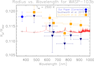
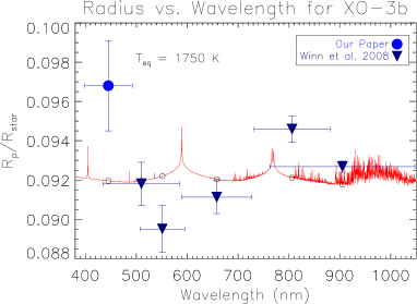
Figure 7: Plot of Rp/$R_{*}$ against wavelength for WASP-103b and XO-3b from this paper and previous literature. Both WASP-103b and XO-3b show variations with wavelength. Other comments are the same as Fig. 6

5.11 XO-3b

XO-3b is a massive planet (11.79$\pm$0.59 $M_{Jup}$) with a large eccentricity (0.26$\pm$ 0.017) detected by the XO survey (Johns-Krull et al. 2008). Further photometric observations have refined the system’s parameters (Winn et al. 2008; Hirano et al. 2011; Machalek et al. 2010; Wong et al. 2014) and Hébrard et al. (2008) found that XO-3’s spin axis is misaligned with XO-3b’s rotation axis.

We observed a transit of XO-3b on 2012 November 30 with the Harris B filter (Fig. 3). We derive physical parameters that are in agreement with previous literature (Tables 5 and 7). Our calculated R_p/R_∗ is 2$\sigma$ larger than the V-band R_p/R_∗ found by Winn et al. (2008). We calculate a refined period with an error decreased by a factor of 13 from the value found by Winn et al. (2008). A non-flat spectrum for R_p/R_∗ is found for XO-3b (Table 9; Fig 7).

6 Discussion

6.1 Wavelength dependence on the transit depth

We find a constant transit depth across optical wavelengths for the TEPs HAT-P-5b, HAT-P-12b, WASP-2b, WASP-24b, and WASP-80b (Fig 6, Table 9). A lack of variation in radius with wavelength could suggest these planets (HAT-P-5b, HAT-P-12b, WASP-2b, WASP-80b) have clouds/hazes in their upper atmospheres (e.g. Seager & Sasselov 2000; Brown 2001; Gibson et al. 2013b; Marley et al. 2013; Kreidberg et al. 2014) or they have an isothermal pressure-temperature profile (Fortney et al., 2006). Mancini et al. (2014) also do not detect a significant variation in WASP-80b’s transit depth with wavelength, and Southworth et al. (2012) finds a relatively flat spectrum of planetary radii for HAT-P-5b with the exception of their observed radius in the U-band (which they suspect is caused by systematic error in their U-band photometry). A flat spectrum for WASP-24b is also found with the exception of one value. Our R-band R_p/R_∗ found for WASP-24b differs by 4$\sigma$ from the previously calculated R_p/R_∗ (Southworth et al. 2014) for that same band. The cause of this is unclear and future observations are needed to investigate. Our results are consistent with other transiting exoplanet observations having a flat spectrum in optical wavelengths (i.e. TrES-3b, Turner et al. 2013; GJ 1214b, Bean et al. 2011; Kreidberg et al. 2014; WASP-29b, Gibson et al. 2013a; Gibson et al. 2013b; HAT-P-19b, Mallonn et al. 2015a; HAT-P-1b, HAT-P-13b, HAT-P-16b, HAT-P-22b, TrES-2b, WASP-33b, WASP-44b, WASP-48b, WASP-77Ab, Turner et al. 2016b).

We find variations in the transit depth with wavelength for CoRoT-12b, HAT-P-33b, HAT-P-37b, WASP-103b, and XO-3b (Fig 6-7, Table 9), which could indicate scattering (i.e. due to aerosols or Rayleigh scattering) or absorption in their atmospheres (e.g. Benneke & Seager 2012; Griffith 2014). Our observation of HAT-P-37b exhibits a smaller transit depth in B-band than the red/near-IR value. Such a variation has only been seen in a recent paper by Evans et al. (2016) where they observe a smaller B-band transit depth than optical in WASP-121b. Evans et al. (2016) believe a possible cause of such a variation is TiO/VO absorption and this may also be the cause of the transit depth variations seen in HAT-P-37b. However, more theoretic modeling is needed to confirm that TiO/VO is in fact the opacity source. Additionally, a smaller near-UV radius was recently observed in the hot Jupiter WASP-1b (Turner et al. 2016b), however, these observations did not observe in the B-band. Future near-UV and blue-band observations are needed for WASP-103b and XO-3b to determine whether the scattering in their atmospheres is due to Rayleigh scattering (Lecavelier Des Etangs et al. 2008; Tinetti et al. 2010; de Wit & Seager 2013; Griffith 2014) since these bands are the only optical wavelengths not affected by strong spectral features. The radius variations in WASP-103b show a consistently larger transit depth in the near-UV and blue than the rest of the optical (this varation is still present when corrected for dilution due the companion star). Such a radius variation may indicate a change in particle size at different altitudes of the planetary atmosphere (e.g. Wakeford & Sing 2015). We find a larger R-band transit depth in HAT-P-33b and CoRoT-12b than their discovery transit depths. Since the R-filter encompasses the $H\alpha$ line (656.281 nm), our observation could be an indication of atmospheric escape such as that observed in the atmospheres of HD 189733b (Jensen et al. 2012; Cauley et al. 2015; Barnes et al. 2016; Cauley et al. 2017a; Cauley et al. 2017b) and HD 209458b (Astudillo-Defru & Rojo, 2013) and predicted (e.g. Christie et al. 2013; Turner et al. 2016a). Follow-up photometry and high-resolution spectroscopy observations are encouraged to confirm all the transit depth variations. These results also agree with observations of other exoplanets not having a flat spectrum (i.e. HD 209458b, Sing et al. 2008; HAT-P-5b, Southworth et al. 2012; GJ 3470b, Nascimbeni et al. 2013; Qatar-2, Mancini et al. 2014; WASP-17b, WASP-39b, HAT-P-1b, WASP-31b, HAT-P-12b, HD189733b, WASP-6b, Sing et al. 2016; CoRoT-1b, TrES-4b, WASP-1b, WASP-12b, WASP-36b, Turner et al. 2016b).

For illustration, the observed R_p/R_∗ differences with wavelength for each target (Table 9) are compared to theoretical predictions (Fortney & Nettelmann 2010) for a model planetary atmosphere (Figure 6–7). The models used are calculated for planets with a 1 $M_{Jup}$, $g_{p}=25ms^{-1}$ or $g_{p}=10ms^{-1}$, base radius of 1.25 $R_{Jup}$ at 10 bar, $T_{eq}$ closest to the measured value for each exoplanet (with model choices of 500, 750, 1000, 1250, 1500, 1750, 2000, 2500 K), and solar metallicity. To provide a best fit to the spectral changes a vertical offset is applied to the model. This comparison is helpful as it illustrates the size of observed variation compared to what the theoretical models predict. However, radiative transfer models calculated for each exoplanet individually are needed to fully understand their transmission spectra.

Finally, no signs of asymmetric transits are seen in the near-UV light curves of HAT-P-5b, WASP-80b, and WASP-103b. This result is consistent with ground-based near-UV observations of 19 other transiting exoplanets (Southworth et al. 2012; Pearson et al. 2014; Turner et al. 2013; Bento et al. 2014; Copperwheat et al. 2013; Zellem et al. 2015; Turner et al. 2016b) that show no evidence of asymmetric transits. Additionally, theoretical modeling by Turner et al. (2016a) using the CLOUDY plasma simulation code showed that asymmetric transits cannot be produced in the broad-band near-UV band regardless of the assumed physical phenomena that could cause absorption (e.g. Vidotto et al. 2010; Lai et al. 2010; Ben-Jaffel & Ballester 2014; Matsakos et al. 2015; Kislyakova et al. 2016).

6.1.1 Variability in the host stars

One of the major assumptions in our interpretation that the planetary atmosphere is the cause of the transit depth variations is that the brightness of the host stars have minimal variability due to stellar activity. The presence of star spots and stellar activity can produce variations in the observed transit depth (e.g. Czesla et al. 2009; Oshagh et al. 2013; Oshagh et al. 2014; Zellem et al. 2015; Zellem et al. 2017). This effect is stronger in the near-UV and blue and can mimic a Rayleigh scattering signature (e.g. Oshagh et al. 2014; McCullough et al. 2014). Additionally, no obvious star spot crossing is seen in our data (Figs. 1-3) with the possible exception of HAT-P-37b (see below).

We estimate how much the transit depth may change due to unocculted spots using the formalization presented by Sing et al. (2011). This method assumes that the spots can be treated as a stellar spectrum but with a lower effective temperature, no surface brightness variation outside the spots, and no plage are present. The effect of these assumptions are a dimming of the star and therefore an increase in the transit depth. Sing et al. (2011) find for HD 189733b that the change in transit depth due to unocculted spots, $\Delta\left(R_{p}/R_{\ast}\right)=2.08\times 10^{-3}/2\left(R_{p}/R_{\ast}\right)$ between 375–400 $\rm{nm}$. Therefore, unocculted spots have minimal influence (assuming our host stars have unocculted spots similar to HD 189733b) on the observed transit depth variations since our final error bars (Table 5) are at least 10 times larger than the influence of these spots (e.g. $\Delta\left[R_{p}/R_{\ast}\right]$ = 0.00014 for HAT-P-37b). Qualitatively, this result is consistent with the study by Llama & Shkolnik (2015) that find that stellar activity similar to the sun has very little effect on the transit depth measured in near-UV to optical wavelengths. Nonetheless, we highly encourage follow-up observations and host star monitoring of all our targets to assess the effect of stellar activity on the observed transit depth variations.

Next, we investigate what effect a star-spot crossing in the light curve of HAT-P-37 would have on its calculated transit depth. In the B-band light curve of HAT-P-37b (Figure 1) there may be a star-spot crossing at a phase range of 0.004–0.008. However, the detected signal is very close to the scatter in the light curve. If we model the light curve without the possible star-spot crossing we find a $\left(R_{p}/R_{\ast}\right)=0.1278\pm 0.0048$, within 1$\sigma$ of the transit depth of the entire light curve (0.1253$\pm 0.0021$). McCullough et al. (2014) present a procedure to estimate the effects of unocculted spots on the transit depth. Their procedure can also be used to estimate the effect of star spot crossings on the transit depth, where instead of unocculted spots increasing the transit depth occulted spots should decrease it. McCullough et al. (2014) find that the change in transit depth due to spots, $\Delta(R_{p}^{2}/R_{\ast}^{2})$, is

$$\Delta\left(\frac{R_{p}^{2}}{R_{\ast}^{2}}\right)=\left(\frac{R_{p}}{R_{\ast}}\right)^{2}\delta\frac{T_{spot}}{T_{\textrm{eff}}},$$ (5)

where $R_{p}/R_{\ast}$ is the unperturbed transit depth, $\delta$ is the fractional area of star spots, and $T_{spot}$ is the temperature of the spot. If we set $\Delta(R_{p}^{2}/R_{\ast}^{2})$ = 3100 ppm (the approximate difference between our B-band and the Sloan-i transit depth; Hartman et al. 2011), then we can estimate $T_{spot}$ and $\delta$. For spot temperatures between 2000–5000 K, we find that $\delta$ would be between 20 - 50 $\%$. Typical values of $\delta$ for solar-like stars is around several $\%$ (e.g. Pont et al. 2008; Sing et al. 2011; McCullough et al. 2014), so our estimated $\delta$ range is extremely high. Due to both these tests, it seems unlikely that the smaller B-band transit depth of HAT-P-37b is due to an occulted star-spot.

7 Conclusions

We observed 11 transiting hot Jupiters (CoRoT-12b, HAT-P-5b, HAT-P-12b, HAT-P-33b, HAT-P-37b, WASP-2b, WASP-24b, WASP-60b, WASP-80b, WASP-103b, XO-3b) from the ground using near-UV and optical filters in order to update their system parameters and constrain their atmospheres. Our observations of CoRoT-12b, HAT-P-37b and WASP-60b are the first follow-up observations of these planets since their discovery and we also obtain the first near-UV light curves of WASP-80b and WASP-103b. We find that HAT-P-5b, HAT-P-12b, WASP-2b, WASP-24b, and WASP-80b exhibit a flat spectrum across the optical wavelengths, suggestive of clouds in their atmospheres. Variation in the transit depths is observed for WASP-103b and XO-3b and may indicate scattering in their atmospheres. Additionally, we observe a smaller B-band transit depth compared to near-IR in HAT-P-37b. Such a variation may be caused by TiO/VO absorption (Evans et al. 2016). We find a larger R-band (which encompasses the H$\alpha$ line) transit depths in HAT-P-33b and CoRoT-12b and this result may indicate possible atmospheric escape. Follow-up photometry and high-resolution spectroscopy observations are encouraged to confirm all the observed transit depth variations since they are only seen at 2-4.6$\sigma$. Our calculated physical parameters agree with previous studies within 1$\sigma$ with a few exceptions (Tables 6–7). For the exoplanets HAT-P-12b, HAT-P-37b, WASP-2b, WASP-24b, WASP-80b, and XO-3b we are able to refine their orbital periods from previous work (Tables 6–7).

References

- Akeson et al. (2013) Akeson R. L., et al., 2013, PASP, 125, 989
- Albrecht et al. (2011) Albrecht S., et al., 2011, ApJ, 738, 50
- Astudillo-Defru & Rojo (2013) Astudillo-Defru N., Rojo P., 2013, A$&$A, 557, A56
- Baglin (2003) Baglin A., 2003, Advances in Space Research, 31, 345
- Bakos et al. (2007) Bakos G. Á., et al., 2007, ApJl, 671, L173
- Bakos et al. (2012) Bakos G. Á., et al., 2012, AJ, 144, 19
- Barnes et al. (2013) Barnes J. W., van Eyken J. C., Jackson B. K., Ciardi D. R., Fortney J. J., 2013, APJ, 774, 53
- Barnes et al. (2016) Barnes J. R., Haswell C. A., Staab D., Anglada-Escudé G., 2016, MNRAS, 462, 1012
- Bean et al. (2011) Bean J. L., et al., 2011, ApJ, 743, 92
- Becker et al. (2013) Becker A. C., Kundurthy P., Agol E., Barnes R., Williams B. F., Rose A. E., 2013, ApJl, 764, L17
- Ben-Jaffel & Ballester (2014) Ben-Jaffel L., Ballester G. E., 2014, ApJl, 785, L30
- Benneke & Seager (2012) Benneke B., Seager S., 2012, ApJ, 753, 100
- Bento et al. (2014) Bento J., et al., 2014, MNRAS, 437, 1511
- Bessell (1979) Bessell M. S., 1979, PASP, 91, 589
- Biddle et al. (2014) Biddle L. I., et al., 2014, MNRAS, 443, 1810
- Borucki et al. (2010) Borucki W. J., et al., 2010, Science, 327, 977
- Braak (2006) Braak C., 2006, Statistics and Computing, 16, 239
- Brown (2001) Brown T. M., 2001, ApJ, 553, 1006
- Bruntt et al. (2006) Bruntt H., Southworth J., Torres G., Penny A. J., Clausen J. V., Buzasi D. L., 2006, A&A, 456, 651
- Carone et al. (2012) Carone L., et al., 2012, A&A, 538, A112
- Carter & Winn (2009) Carter J. A., Winn J. N., 2009, ApJ, 704, 51
- Castelli & Kurucz (2004) Castelli F., Kurucz R. L., 2004, ArXiv Astrophysics e-prints, astro-ph/0405087
- Cauley et al. (2015) Cauley P. W., Redfield S., Jensen A. G., Barman T., Endl M., Cochran W. D., 2015, ApJ, 810, 13
- Cauley et al. (2017a) Cauley P. W., Redfield S., Jensen A. G., 2017a, AJ, 153, 185
- Cauley et al. (2017b) Cauley P. W., Redfield S., Jensen A. G., 2017b, AJ, 153, 217
- Charbonneau et al. (2000) Charbonneau D., Brown T. M., Latham D. W., Mayor M., 2000, ApJl, 529, L45
- Charbonneau et al. (2002) Charbonneau D., Brown T. M., Noyes R. W., Gilliland R. L., 2002, ApJ, 568, 377
- Charbonneau et al. (2007) Charbonneau D., Brown T. M., Burrows A., Laughlin G., 2007, Protostars and Planets V, pp 701–716
- Christie et al. (2013) Christie D., Arras P., Li Z.-Y., 2013, ApJ, 772, 144
- Ciardi et al. (2015) Ciardi D. R., Beichman C. A., Horch E. P., Howell S. B., 2015, ApJ, 805, 16
- Claret & Bloemen (2011) Claret A., Bloemen S., 2011, A&A, 529, A75
- Collier Cameron et al. (2007) Collier Cameron A., et al., 2007, MNRAS, 375, 951
- Copperwheat et al. (2013) Copperwheat C. M., et al., 2013, MNRAS, 434, 661
- Czesla et al. (2009) Czesla S., Huber K. F., Wolter U., Schröter S., Schmitt J. H. M. M., 2009, A&A, 505, 1277
- Daemgen et al. (2009) Daemgen S., Hormuth F., Brandner W., Bergfors C., Janson M., Hippler S., Henning T., 2009, A&A, 498, 567
- Dittmann et al. (2009a) Dittmann J. A., Close L. M., Green E. M., Scuderi L. J., Males J. R., 2009a, ApJl, 699, L48
- Dittmann et al. (2009b) Dittmann J. A., Close L. M., Green E. M., Fenwick M., 2009b, ApJ, 701, 756
- Dittmann et al. (2010) Dittmann J. A., Close L. M., Scuderi L. J., Morris M. D., 2010, ApJ, 717, 235
- Dittmann et al. (2012) Dittmann J. A., Close L. M., Scuderi L. J., Turner J., Stephenson P. C., 2012, New Astron., 17, 438
- Eastman et al. (2010) Eastman J., Siverd R., Gaudi B. S., 2010, PASP, 122, 935
- Eastman et al. (2013) Eastman J., Gaudi B. S., Agol E., 2013, PASP, 125, 83
- Evans et al. (2016) Evans T. M., et al., 2016, preprint (ArXiv:1604.02310),
- Ford (2006) Ford E. B., 2006, ApJ, 642, 505
- Fortney & Nettelmann (2010) Fortney J. J., Nettelmann N., 2010, Space Sci. Rev., 152, 423
- Fortney et al. (2006) Fortney J. J., Cooper C. S., Showman A. P., Marley M. S., Freedman R. S., 2006, ApJ, 652, 746
- Fortney et al. (2007) Fortney J. J., Marley M. S., Barnes J. W., 2007, ApJ, 659, 1661
- Fukui et al. (2014) Fukui A., et al., 2014, ApJ, 790, 108
- Gelman & Rubin (1992) Gelman A., Rubin D. B., 1992, Statist.Sci., 7, 457
- Gibson et al. (2013a) Gibson N. P., Aigrain S., Barstow J. K., Evans T. M., Fletcher L. N., Irwin P. G. J., 2013a, MNRAS, 428, 3680
- Gibson et al. (2013b) Gibson N. P., Aigrain S., Barstow J. K., Evans T. M., Fletcher L. N., Irwin P. G. J., 2013b, MNRAS, 436, 2974
- Gillon et al. (2010) Gillon M., et al., 2010, A&A, 520, A97
- Gillon et al. (2014) Gillon M., et al., 2014, A&A, 562, L3
- Griffith (2014) Griffith C. A., 2014, Royal Society of London Philosophical Transactions Series A, 372, 30086
- Hartman et al. (2009) Hartman J. D., et al., 2009, ApJ, 706, 785
- Hartman et al. (2011) Hartman J. D., et al., 2011, ApJ, 742, 59
- Hébrard et al. (2008) Hébrard G., et al., 2008, A&A, 488, 763
- Hébrard et al. (2013) Hébrard G., et al., 2013, A&A, 549, A134
- Henry et al. (2000) Henry G. W., Marcy G. W., Butler R. P., Vogt S. S., 2000, ApJL, 529, L41
- Hirano et al. (2011) Hirano T., Narita N., Sato B., Winn J. N., Aoki W., Tamura M., Taruya A., Suto Y., 2011, PASJ, 63, L57
- Holman & Murray (2005) Holman M. J., Murray N. W., 2005, Science, 307, 1288
- Holman et al. (2010) Holman M. J., et al., 2010, Science, 330, 51
- Howell et al. (2014) Howell S. B., et al., 2014, PASP, 126, 398
- Hubbard et al. (2001) Hubbard W. B., Fortney J. J., Lunine J. I., Burrows A., Sudarsky D., Pinto P., 2001, ApJ, 560, 413
- Husnoo et al. (2012) Husnoo N., Pont F., Mazeh T., Fabrycky D., Hébrard G., Bouchy F., Shporer A., 2012, MNRAS, 422, 3151
- Jensen et al. (2012) Jensen A. G., Redfield S., Endl M., Cochran W. D., Koesterke L., Barman T., 2012, ApJ, 751, 86
- Johns-Krull et al. (2008) Johns-Krull C. M., et al., 2008, ApJ, 677, 657
- Kislyakova et al. (2016) Kislyakova K. G., et al., 2016, MNRAS, 461, 988
- Kreidberg et al. (2014) Kreidberg L., et al., 2014, Nat, 505, 69
- Lai et al. (2010) Lai D., Helling C., van den Heuvel E. P. J., 2010, ApJ, 721, 923
- Lecavelier Des Etangs et al. (2008) Lecavelier Des Etangs A., Pont F., Vidal-Madjar A., Sing D., 2008, A&A, 481, L83
- Lee et al. (2012) Lee J. W., Youn J.-H., Kim S.-L., Lee C.-U., Hinse T. C., 2012, AJ, 143, 95
- Lendl et al. (2017) Lendl M., Cubillos P. E., Hagelberg J., Müller A., Juvan I., Fossati L., 2017, preprint, (arXiv:1708.05737)
- Line et al. (2013) Line M. R., Knutson H., Deming D., Wilkins A., Desert J.-M., 2013, ApJ, 778, 183
- Llama & Shkolnik (2015) Llama J., Shkolnik E. L., 2015, ApJ, 802, 41
- Machalek et al. (2010) Machalek P., Greene T., McCullough P. R., Burrows A., Burke C. J., Hora J. L., Johns-Krull C. M., Deming D. L., 2010, ApJ, 711, 111
- Maciejewski et al. (2016) Maciejewski G., et al., 2016, AcA, 66, 55
- Mallonn et al. (2015a) Mallonn M., et al., 2015a, A&A, 580, A60
- Mallonn et al. (2015b) Mallonn M., et al., 2015b, A$&$A, 583, A138
- Mancini et al. (2014) Mancini L., et al., 2014, A&A, 562, A126
- Mandel & Agol (2002) Mandel K., Agol E., 2002, ApJl, 580, L171
- Markwardt (2009) Markwardt C. B., 2009, in Bohlender D. A., Durand D., Dowler P., eds, Astronomical Society of the Pacific Conference Series Vol. 411, Astronomical Data Analysis Software and Systems XVIII. p. 251 (arXiv:0902.2850)
- Marley et al. (2013) Marley M. S., Ackerman A. S., Cuzzi J. N., Kitzmann D., 2013, Clouds and Hazes in Exoplanet Atmospheres. pp 367–391, doi:10.2458/azu˙uapress˙9780816530595-ch15
- Matsakos et al. (2015) Matsakos T., Uribe A., Königl A., 2015, A$&$A, 578, A6
- McCullough et al. (2014) McCullough P. R., Crouzet N., Deming D., Madhusudhan N., 2014, ApJ, 791, 55
- Miralda-Escudé (2002) Miralda-Escudé J., 2002, ApJ, 564, 1019
- Moutou et al. (2013) Moutou C., et al., 2013, Icarus, 226, 1625
- Nascimbeni et al. (2013) Nascimbeni V., Piotto G., Pagano I., Scandariato G., Sani E., Fumana M., 2013, A&A, 559, A32
- Ngo et al. (2016) Ngo H., et al., 2016, ApJ, 827, 8
- Oshagh et al. (2013) Oshagh M., Santos N. C., Boisse I., Boué G., Montalto M., Dumusque X., Haghighipour N., 2013, A&A, 556, A19
- Oshagh et al. (2014) Oshagh M., Santos N. C., Ehrenreich D., Haghighipour N., Figueira P., Santerne A., Montalto M., 2014, A&A, 568, A99
- Pearson et al. (2014) Pearson K. A., Turner J. D., Sagan T. G., 2014, New Astron., 27, 102
- Pollacco et al. (2006) Pollacco D. L., et al., 2006, PASP, 118, 1407
- Pont et al. (2006) Pont F., Zucker S., Queloz D., 2006, MNRAS, 373, 231
- Pont et al. (2008) Pont F., Knutson H., Gilliland R. L., Moutou C., Charbonneau D., 2008, MNRAS, 385, 109
- Press et al. (1992) Press W. H., Teukolsky S. A., Vetterling W. T., Flannery B. P., 1992, Numerical recipes in FORTRAN. The art of scientific computing
- Saar et al. (1998) Saar S. H., Butler R. P., Marcy G. W., 1998, ApJl, 498, L153
- Sada & Ramón-Fox (2016) Sada P. V., Ramón-Fox F. G., 2016, PASP, 128, 024402
- Sada et al. (2012) Sada P. V., et al., 2012, PASP, 124, 212
- Safronov (1972) Safronov V. S., 1972, Evolution of the protoplanetary cloud and formation of the earth and planets.
- Salz et al. (2015) Salz M., Schneider P. C., Czesla S., Schmitt J. H. M. M., 2015, A&A, 576, A42
- Schwarz (1978) Schwarz G., 1978, The Annals of Statistics, 6, 461
- Scuderi et al. (2010) Scuderi L. J., Dittmann J. A., Males J. R., Green E. M., Close L. M., 2010, ApJ, 714, 462
- Seager (2011) Seager S., 2011, Exoplanets. Univ. of Arizona Press, Tucson, AZ
- Seager & Sasselov (2000) Seager S., Sasselov D. D., 2000, ApJ, 537, 916
- Sedaghati et al. (2017) Sedaghati E., Boffin H. M. J., Delrez L., Gillon M., Csizmadia S., Smith A. M. S., Rauer H., 2017, MNRAS, 468, 3123
- Simpson et al. (2011) Simpson E. K., et al., 2011, MNRAS, 414, 3023
- Sing et al. (2008) Sing D. K., Vidal-Madjar A., Désert J.-M., Lecavelier des Etangs A., Ballester G., 2008, ApJ, 686, 658
- Sing et al. (2011) Sing D. K., et al., 2011, MNRAS, 416, 1443
- Sing et al. (2016) Sing D. K., et al., 2016, Natur, 529, 59
- Sokov et al. (2012) Sokov E. N., et al., 2012, Astronomy Letters, 38, 180
- Southworth (2008) Southworth J., 2008, MNRAS, 386, 1644
- Southworth (2010) Southworth J., 2010, MNRAS, 408, 1689
- Southworth & Evans (2016) Southworth J., Evans D. F., 2016, MNRAS, 463, 37
- Southworth et al. (2007a) Southworth J., Wheatley P. J., Sams G., 2007a, MNRAS, 379, L11
- Southworth et al. (2007b) Southworth J., Bruntt H., Buzasi D. L., 2007b, A&A, 467, 1215
- Southworth et al. (2010) Southworth J., et al., 2010, MNRAS, 408, 1680
- Southworth et al. (2012) Southworth J., Mancini L., Maxted P. F. L., Bruni I., Tregloan-Reed J., Barbieri M., Ruocco N., Wheatley P. J., 2012, MNRAS, 422, 3099
- Southworth et al. (2014) Southworth J., et al., 2014, MNRAS, 444, 776
- Southworth et al. (2015) Southworth J., et al., 2015, MNRAS, 447, 711
- Street et al. (2010) Street R. A., et al., 2010, ApJ, 720, 337
- Teske et al. (2013) Teske J. K., Turner J. D., Mueller M., Griffith C. A., 2013, MNRAS, 431, 1669
- Tinetti et al. (2010) Tinetti G., Deroo P., Swain M. R., Griffith C. A., Vasisht G., Brown L. R., Burke C., McCullough P., 2010, ApJ, 712, L139
- Torres et al. (2008) Torres G., Winn J. N., Holman M. J., 2008, ApJ, 677, 1324
- Triaud et al. (2010) Triaud A. H. M. J., et al., 2010, A&A, 524, A25
- Triaud et al. (2013) Triaud A. H. M. J., et al., 2013, A&A, 551, A80
- Triaud et al. (2015) Triaud A. H. M. J., et al., 2015, MNRAS, 450, 2279
- Turner et al. (2013) Turner J. D., et al., 2013, MNRAS, 428, 678
- Turner et al. (2016a) Turner J. D., Christie D., Arras P., Johnson R. E., Schmidt C., 2016a, MNRAS, 458, 3880
- Turner et al. (2016b) Turner J. D., et al., 2016b, MNRAS, 459, 789
- Vidotto et al. (2010) Vidotto A. A., Jardine M., Helling C., 2010, ApJl, 722, L168
- Wakeford & Sing (2015) Wakeford H. R., Sing D. K., 2015, A$&$A, 573, A122
- Wang et al. (2017) Wang Y.-H., et al., 2017, AJ, 154, 49
- Winn (2010) Winn J. N., 2010, preprint (arXiv:1001.2010),
- Winn et al. (2008) Winn J. N., et al., 2008, ApJ, 683, 1076
- Wöllert & Brandner (2015) Wöllert M., Brandner W., 2015, A$&$A, 579, A129
- Wong et al. (2014) Wong I., et al., 2014, ApJ, 794, 134
- Wright et al. (2011) Wright J. T., et al., 2011, PASP, 123, 412
- Zellem et al. (2015) Zellem R. T., et al., 2015, ApJ, 810, 11
- Zellem et al. (2017) Zellem R. T., et al., 2017, ApJ, 844, 27
- Zhang et al. (2011) Zhang J.-C., Cao C., Song N., Wang F.-G., Zhang X.-T., 2011, Chin. Astron. Astrophys., 35, 409
- de Wit & Seager (2013) de Wit J., Seager S., 2013, Science, 342, 1473