Effective-field theory analysis of the $\tau^{-}\to\eta^{(\prime)}\pi^{-}\nu_{\tau}$ decays

Abstract

The rare $\tau^{-}\to\eta^{(\prime)}\pi^{-}\nu_{\tau}$ decays, which are suppressed by $G$-parity in the Standard Model (SM), can be sensitive to the effects of new interactions. We study the sensitivity of different observables of these decays in the framework of an effective field theory that includes the most general interactions between SM fields up to dimension six, assuming massless neutrinos. Owing to the strong suppression of the SM isospin breaking amplitudes, we find that the different observables would allow to set constraints on scalar interactions that are stronger than those coming from other low-energy observables.

I Introduction

Rare processes are suppressed decay modes of particles originated by approximate symmetries of the SM. They provide an ideal place to look for new physics because their suppressed amplitudes can be of similar size as the (virtual) effects due to new particles and interactions. It turns out that having a good control of SM uncertainties is crucial to disentangle the effects of such New Physics contributions in precision measurements at flavor factories.

In this paper we study the rare $\tau^{-}\to\eta^{(\prime)}\pi^{-}\nu_{\tau}$ decays, which will be forbidden if $G-$parity Lee:1956sw were an exact symmetry of the SM ($G=Ce^{i\pi I_{2}}$, with $C$ the charge conjugation operation and $I_{i}$ the components of the isospin rotation operators). This process was suggested long ago Leroy:1977pq as a clean test of Second Class Currents (SCC) following a classification proposed by Weinberg Weinberg:1958ut for strangeness-conserving interactions. According to this classification, SCC must have quantum numbers $PG(-1)^{J}=-1$ as opposite to (first class) currents in the SM which have $PG(-1)^{J}=+1$. Since isospin is only a partial symmetry of strong interactions, $G-$parity gets broken by the $u-d$ quark mass and electric charge differences and $\tau^{-}\to\eta^{(\prime)}\pi^{-}\nu_{\tau}$ decays can occur, although at a suppressed rate. This suppression makes interesting these decays to study the effects of genuine SCC, (i. e. not induced by isospin breaking effects), such as the ones induced by the exchange of charged Higgs Branco:2011iw ; Jung:2010ik or leptoquark bosons Becirevic:2016yqi  . We study these processes in the framework of an effective Lagrangian where the effects of New Physics are encoded in the most general Lagrangian involving dimension-six operators with left-handed neutrino fields.

Our study focuses on different partial and total integrated observables on $\tau^{-}\to\eta^{(\prime)}\pi^{-}\nu_{\tau}$ decays, as they can exhibit different sensitivities to the various effective couplings. Previous studies (including specific beyond the SM approaches) have focused mainly in the estimates of the branching fractions in the $10^{-5}\sim 10^{-6}$ ($10^{-6}\sim 10^{-8}$) range for the $\eta$ ($\eta^{\prime}$) decay channels BRs , as well as on the invariant mass distribution Vienna ; Orsay ; Escribano:2016ntp . An important source of uncertainty in most of these estimates arises from the predictions used for the scalar form factor contribution. Of course, a good knowledge of the scalar form factor is necessary in order to assess the possible contributions of beyond SM effects. Once the $\tau^{-}\to\eta^{(\prime)}\pi^{-}\nu_{\tau}$ decays have been observed at future superflavor factories, we expect that detailed studies of the different observables will be very useful to disentangle the New Physics effects from the SM isospin-violating contributions .

The current experimental limits for the SCC tau branching ratios of $\tau^{-}\to\eta\pi^{-}\nu$ are: Br $<9.9\times 10^{-5}$, $95\%$ CL (BaBar delAmoSanchez:2010pc ), $<7.3\times 10^{-5}$, $90\%$ CL (Belle Hayasaka:2009zz ) and $<1.4\times 10^{-4}$, $95\%$ CL (CLEO Bartelt:1996iv ) collaborations, respectively. Those upper limits lie very close to the SM estimates based on isospin breaking BRs ; Vienna ; Orsay ; Escribano:2016ntp . The corresponding BaBar limit for the $\tau^{-}\to\eta^{\prime}\pi^{-}\nu_{\tau}$ decays is $<7.2\cdot 10^{-6}$, $95\%$ CL Aubert:2008nj , while Belle obtained $<4.6\cdot 10^{-6}$, $90\%$ CL Hayasaka:2009zz (CLEO set the earlier upper bound $7.4\times 10^{-5}$, $90\%$CL Bergfeld:1997zt ). Future experiments at the intensity frontier like Belle II Abe:2010gxa , which will accumulate $4.5\times 10^{10}$ tau lepton pairs in the full dataset, are expected to provide the first measurements of the $\tau^{-}\to\eta^{(\prime)}\pi^{-}\nu_{\tau}$ SCC decays B2TIPReport .

This paper is organized as follows: in section II we set our conventions for the effective field theory analysis of the $\tau^{-}\to\nu_{\tau}\bar{u}d$ decays, to be used in the remainder of the article. In section III, we discuss the different effective weak currents contributing to the considered decays and define their corresponding hadronic form factors. The tensor form factor within low-energy QCD is computed in section IV. In section V we discuss the different observables that can help elucidating non-SM contributions to the $\tau^{-}\to\eta^{(\prime)}\pi^{-}\nu_{\tau}$ decays and in section VI we state our conclusions.

II Effective theory analysis of $\tau{{}^{-}}\to\nu_{\tau}\bar{u}d$

The effective Lagrangian with $SU(2)_{L}\otimes U(1)$ invariant dimension six operators at the weak scale contributing to low-energy charged current processes can be written as Bhattacharya:2011qm ; Cirigliano:2009wk

$${\cal L}^{(\rm{eff})}={\cal L}_{\rm{SM}}+\frac{1}{\Lambda^{2}}\sum_{i}~{}\alpha_{i}O_{i}\ \longrightarrow\ {\cal L}_{\rm{SM}}+\frac{1}{v^{2}}\,\sum_{i}\,\hat{\alpha}_{i}~{}O_{i}\,,$$ (1)

with $\hat{\alpha}_{i}=(v^{2}/\Lambda^{2})\alpha_{i}$ the dimensionless new physics couplings, which are $O(10^{-3})$ for an scale $\Lambda\sim 1\ {\rm TeV}$.

The low-scale $O(1\ {\rm GeV})$ effective Lagrangian for semi-leptonic ($\ell\,=\,e,\,\mu,\,\tau$) strangeness and lepton-flavor conserving transitions involving only left-handed neutrino fields is given by (subscripts $L(R)$ refer to left-handed (right-handed) chiral projections)

$${\cal L}_{\rm CC} = \frac{-4G_{F}}{\sqrt{2}}\,V_{ud}\,\Bigg{[}\Big{(}1+[v_{L}]_{\ell\ell}\Big{)}\ \bar{\ell}_{L}\gamma_{\mu}\nu_{\ell L}\ \bar{u}_{L}\gamma^{\mu}d_{L}\ +\ [v_{R}]_{\ell\ell}\ \bar{\ell}_{L}\gamma_{\mu}\nu_{\ell L}\ \bar{u}_{R}\gamma^{\mu}d_{R}$$ (2)

$$+ [s_{L}]_{\ell\ell}\ \bar{\ell}_{R}\nu_{\ell L}\ \bar{u}_{R}d_{L}\ +\ [s_{R}]_{\ell\ell}\ \bar{\ell}_{R}\nu_{\ell L}\ \bar{u}_{L}d_{R}$$

$$+ [t_{L}]_{\ell\ell}\ \bar{\ell}_{R}\sigma_{\mu\nu}\nu_{\ell L}\ \bar{u}_{R}\sigma^{\mu\nu}d_{L}\Bigg{]}~{}+~{}{\rm h.c.}~{},$$

where $G_{F}$ stands for the tree-level definition of the Fermi constant, $\sigma^{\mu\nu}\equiv i[\gamma^{\mu},\gamma^{\nu}]/2$, and $v_{L}=v_{R}=s_{L}=s_{R}=t_{L}=0$ gives the SM Lagrangian. In the Lagrangian above, as usual, Higgs, $W^{\pm}$, and $Z$ boson degrees of freedom have been integrated out, as well as $c$, $b$ and $t$ quarks. Since we will be considering only CP-even observables, the effective couplings $v_{L,R}$, $s_{L,R}$, and $t_{L}$ characterizing New Physics can be taken real.

In terms of equivalent effective couplings ($\epsilon_{L,R}=v_{L,R},\ \epsilon_{S}=s_{L}+s_{R},\ \epsilon_{P}=s_{L}-s_{R}$ and $\epsilon_{T}=t_{L}$) we have the following form of the semileptonic effective Lagrangian (particularized for $\ell=\tau$):

$${\cal L}_{\rm CC} = -\frac{G_{F}V_{ud}}{\sqrt{2}}\,\Big{(}1+\epsilon_{L}+\epsilon_{R}\Big{)}\Bigg{[}\bar{\tau}\gamma_{\mu}(1-\gamma_{5})\nu_{\tau}\cdot\bar{u}\Big{[}\gamma^{\mu}\ -\ \big{(}1-2\widehat{\epsilon}_{R}\big{)}\gamma^{\mu}\gamma_{5}\Big{]}d$$ (3)

$$+ \bar{\tau}(1-\gamma_{5})\nu_{\tau}\cdot\bar{u}\Big{[}\widehat{\epsilon}_{S}-\widehat{\epsilon}_{P}\gamma_{5}\Big{]}d+2\widehat{\epsilon}_{T}\,\bar{\tau}\sigma_{\mu\nu}(1-\gamma_{5})\nu_{\tau}\cdot\bar{u}\sigma^{\mu\nu}d\Bigg{]}+{\rm h.c.},\ \ \ \ \$$

where $\widehat{\epsilon_{i}}\equiv\epsilon_{i}/(1+\epsilon_{L}+\epsilon_{R})$ for $i=R,S,P,T$. This factorized form is useful as long as conveniently normalized rates allow to cancel the overall factor $(1+\epsilon_{L}+\epsilon_{R})$. Keeping terms linear in the small effective couplings, the $\widehat{\epsilon}_{i}$’s reduce to the expression in Ref. Bhattacharya:2011qm .

III Semileptonic $\tau$ decay amplitude

Let us consider the semileptonic $\tau^{-}(p)\to\eta^{(\prime)}(p_{\eta})\pi^{-}(p_{\pi})\nu_{\tau}(p^{\prime})$ decays. Owing to the parity of pseudoscalar mesons, only the vector, scalar and tensor currents give a non-zero contribution to the decay amplitude, which reads :

$${\cal M} = {\cal M}_{V}+{\cal M}_{S}+{\cal M}_{T}$$ (4)

$$= \frac{G_{F}V_{ud}\sqrt{S_{EW}}}{\sqrt{2}}(1+\epsilon_{L}+\epsilon_{R})\,\left[L_{\mu}H^{\mu}+\widehat{\epsilon}_{S}LH+2\widehat{\epsilon}_{T}L_{\mu\nu}\,H^{\mu\nu}\right],$$

where we have defined the following leptonic currents

$$L_{\mu} = \bar{u}(p^{\prime})\gamma_{\mu}(1-\gamma_{5})u(p),$$

$$L = \bar{u}(p^{\prime})(1+\gamma_{5})u(p),$$ (5)

$$L_{\mu\nu} = \bar{u}(p^{\prime})\sigma_{\mu\nu}(1+\gamma_{5})u(p),$$

In eq. (4) we have defined the following vector, scalar and tensor hadronic matrix elements

$$H^{\mu} = {\langle\eta^{(\prime)}\pi^{-}}|\bar{d}\gamma^{\mu}u{|0\rangle}=c_{V}Q^{\mu}F_{+}(s)+c_{S}\frac{\Delta^{QCD}_{K^{0}K^{+}}}{s}q^{\mu}F_{0}(s),$$ (6)

$$H = {\langle\eta^{(\prime)}\pi^{-}|}\bar{d}u{|0\rangle}=F_{S}(s),$$ (7)

$$H^{\mu\nu} = {\langle\eta^{(\prime)}\pi^{-}|}\bar{d}\sigma^{\mu\nu}u{|0\rangle}=iF_{T}(s)(p_{\eta}^{\mu}p_{\pi}^{\nu}-p_{\pi}^{\mu}p_{\eta}^{\nu}),$$ (8)

where we have defined $q^{\mu}=(p_{\eta^{(\prime)}}+p_{\pi})^{\mu}$, $Q^{\mu}=(p_{\eta^{(\prime)}}-p_{\pi})^{\mu}+(\Delta_{\pi^{-}\eta^{(\prime)}}/s)q^{\mu}$, $s=q^{2}$ and $\Delta_{ij}\equiv m_{i}^{2}-m_{j}^{2}$, $\Delta^{QCD}_{K^{0}K^{+}}={m_{K^{0}}}^{2}-m_{K^{+}}^{2}+m_{\pi^{+}}^{2}-m_{\pi{{}^{0}}}^{2}$; the constants $c_{S}=\sqrt{\frac{2}{3}},~{}c_{V}=\sqrt{2}$, denote Clebsch-Gordan flavor coefficients. In the $\eta^{\prime}$ case $c_{S}=\frac{2}{\sqrt{3}}$ ($c_{V}$ remains to be $\sqrt{2}$). For simplicity we have not written the labels in the $F_{+,0,S,T}$ form factors, which are different for specific hadronic channels.

The divergence of the vector current relates the $F_{S}(s)$ and $F_{0}(s)$ form factors via

$$F_{S}(s)=c_{S}\frac{\Delta^{QCD}_{K^{0}K^{+}}}{(m_{d}-m_{u})}F_{0}(s)\,.$$ (9)

Since ChPT

$$\frac{\Delta^{QCD}_{K^{0}K^{+}}}{(m_{d}-m_{u})}\,=\,B\left(1-\frac{1}{4}\frac{m_{u}-m_{d}}{m_{s}-\hat{m}}\right)\sim B\,,$$ (10)

where $\hat{m}\equiv(m_{u}+m_{d})/2$ and $BF^{2}=<0|\bar{q}q|0>\sim-(270$ MeV$)^{3}$ Aoki:2016frl , it is seen –by using $F\sim 92$ MeV– that $B\sim M_{\tau}$. Thus, $F_{S}(s)$ basically inherits the strong isospin suppression of $F_{0}(s)$.

Observe that the scalar contribution in eq. (7) can be ‘absorbed’ into the vector current amplitude by using the Dirac equation $L=L_{\mu}q^{\mu}/M_{\tau}$ and eq. (9). This can be achieved by replacing

$$c^{S}\frac{\Delta_{K^{0}K^{+}}^{QCD}}{s}\ \longrightarrow\ c^{S}\frac{\Delta_{K^{0}K^{+}}^{QCD}}{s}\left[1+\frac{s\widehat{\epsilon}_{S}}{m_{\tau}(m_{d}-m_{u})}\right]\ ,$$ (11)

in the second term of eq. (6). We will see in the next section that the remaining contribution to eq. (4), given by the tensor current (${\cal M}_{T}$), is also suppressed in low-energy QCD.

IV Hadronization of the tensor current

The hadronization of the tensor current, eq. (8), is one of the most difficult inputs to be reliably estimated. In the tau lepton decays under consideration, the momentum transfer ranges within $(m_{\eta^{(\prime)}}+m_{\pi})^{2}\leq s\leq M_{\tau}^{2}$, which is the kinematic region populated by light resonances. Here we will neglect the $s$-dependence, namely $F_{T}^{\pi\eta^{(\prime)}}(s)=F_{T}^{\pi\eta^{(\prime)}}(0)\equiv F_{T}^{\pi\eta^{(\prime)}}$, and we will estimate its value using Chiral Perturbation Theory Weinberg:1978kz ; Gasser:1983yg ; Gasser:1984gg ; Colangelo:1999kr . We do not consider tensor current contributions at the next-to-leading chiral order in order to keep predictability.

A comment is in order with respect to neglecting resonance contributions in the hadronization of the tensor current, as it couples to the $J^{PC}=1^{--}$ resonances, being the $\rho(770)$ its lightest representative. In principle, one should expect a contribution from these resonances to the considered decays, providing an energy-dependence to $F_{T}$ and increasing its effect in the observables that we study. The $\rho(770)$ will contribute very little to the $\eta^{\prime}\pi$ decay mode, owing to kinematical constraints, and the contributions of $\rho(1450)$ and $\rho(1700)$ will be damped by phase space and their wide widths. Thus, it is quite justified to assume $F_{T}^{\pi\eta^{\prime}}(s)=F_{T}^{\pi\eta^{\prime}}(0)\equiv F_{T}^{\pi\eta^{\prime}}$. Our previous reasoning does not apply to the vector resonance contribution to $F_{T}^{\pi\eta}(s)$, however. It is predicted by large-$N_{C}$ arguments that vector resonances couple to the tensor current with a strength only a factor $1/\sqrt{2}$ smaller than to the vector current Cata:2008zc (which is also supported by lattice evaluations Becirevic:2003pn ; Braun:2003jg ; Donnellan:2007xr ). Consequently, the $\rho(770)$ contribution to $F_{T}^{\pi\eta}(s)$ should not be negligible (the vector current contribution of the $\rho(770)$ state to the $\tau^{-}\to\eta\pi^{-}\nu_{\tau}$ branching ratio is $\sim 1/6$, according to Ref. Escribano:2016ntp ). As a result, our limits on the allowed values of $\widehat{\epsilon_{T}}$ obtained from the $\pi\eta$ decay mode, which are presented in the next section, could be made stronger including this missing contribution. However, as we will see, the main point of this article is that $\tau^{-}\to\eta^{(\prime)}\pi^{-}\nu_{\tau}$ decays are competitive setting limits on non-standard scalar interactions in charged current decays, while they are not in tensor interactions . This main conclusion is not affected by our assumption $F_{T}^{\pi\eta}(s)=F_{T}^{\pi\eta}(0)\equiv F_{T}^{\pi\eta}$. Therefore our analyses (right panel in figures 5 and 6) involving the tensor source with a constant form factor should be simply viewed as a benchmark to compare with those with the scalar source, and not as a full fledged and theoretically sound computation.

According to Ref. Cata:2007ns , there are only four operators at the leading chiral order, $\mathcal{O}(p^{4})$, that include the tensor current. Only the operator with coefficient $\Lambda_{2}$ contributes to the decays we are considering :

$$\mathcal{L}=\Lambda_{1}\left\langle t_{+}^{\mu\nu}f_{+\,\mu\nu}\right\rangle-i\Lambda_{2}\left\langle t_{+}^{\mu\nu}u_{\mu}u_{\nu}\right\rangle+...\,$$ (12)

where $t_{+}^{\mu\nu}=u^{\dagger}t^{\mu\nu}u^{\dagger}+u{t^{\mu\nu}}^{\dagger}u$ and $\left\langle...\right\rangle$ stands for a trace in flavor space. The chiral tensors entering eq. (12) are $u_{\mu}=i\left[u^{\dagger}(\partial_{\mu}-ir_{\mu})u-u(\partial_{\mu}-i\ell_{\mu})u^{\dagger}\right]$, including the left- and right-handed sources $\ell_{\mu}$ and $r_{\mu}$, the (chiral) tensor sources, $t^{\mu\nu}$ and its adjoint; and $f_{+}^{\mu\nu}=uF_{L}^{\mu\nu}u^{\dagger}+u^{\dagger}F_{R}^{\mu\nu}u$, including the field-strength tensors for $\ell_{\mu}$ and $r_{\mu}$.

The non-linear representation of the pseudoGoldstone bosons is given by $u=\mathrm{exp}\left\{\frac{i}{\sqrt{2}F}\phi\right\}$, where

$$\phi=\begin{pmatrix}\frac{\pi^{3}+\eta_{q}}{\sqrt{2}}&\pi^{+}&K^{+}\\ \pi^{-}&\frac{-\pi^{3}+\eta_{q}}{\sqrt{2}}&K^{0}\\ K^{-}&\overline{K^{0}}&\eta_{s}\end{pmatrix}\,,$$

with $\eta_{q}=C_{q}\eta+C_{q^{\prime}}\eta^{\prime}$ and $\eta_{s}=-C_{s}\eta+C_{s^{\prime}}\eta^{\prime}$ the light and strange quark components of the $\eta,\ \eta^{\prime}$ mesons, respectively ($\pi^{3}$ is the pseudoGoldstone having the flavor quantum numbers of the $\lambda_{3}$ Gell-Mann matrix, which coincides with the $\pi^{0}$ neglecting isospin breaking). These constants describing the $\eta-\eta^{\prime}$ mixing are given by ChPTLargeN

$$C_{q} \equiv \frac{F}{\sqrt{3}\mathrm{cos}(\theta_{8}-\theta_{0})}\left(\frac{\mathrm{cos}\theta_{0}}{f_{8}}-\frac{\sqrt{2}\mathrm{sin}\theta_{8}}{f_{0}}\right)\,,\quad C_{q^{\prime}}\equiv\frac{F}{\sqrt{3}\mathrm{cos}(\theta_{8}-\theta_{0})}\left(\frac{\sqrt{2}\mathrm{cos}\theta_{8}}{f_{0}}+\frac{\mathrm{sin}\theta_{0}}{f_{8}}\right)\,,$$

$$C_{s} \equiv \frac{F}{\sqrt{3}\mathrm{cos}(\theta_{8}-\theta_{0})}\left(\frac{\sqrt{2}\mathrm{cos}\theta_{0}}{f_{8}}+\frac{\mathrm{sin}\theta_{8}}{f_{0}}\right)\,,\quad C_{s^{\prime}}\equiv\frac{F}{\sqrt{3}\mathrm{cos}(\theta_{8}-\theta_{0})}\left(\frac{\mathrm{cos}\theta_{8}}{f_{0}}-\frac{\sqrt{2}\mathrm{sin}\theta_{0}}{f_{8}}\right)\,,$$ (13)

and the corresponding values of the pairs of decay constants and mixing angles are 2anglemixing

$$\theta_{8}\,=\,\left(-21.2\pm 1.6\right)^{\circ},\quad\theta_{0}\,=\,\left(-9.2\pm 1.7\right)^{\circ},\quad f_{8}\,=\,\left(1.26\pm 0.04\right)F,\quad f_{0}\,=\,\left(1.17\pm 0.03\right)F\,$$ (14)

with $F\sim 92.2$ MeV being the pion decay constant.

We recall Cata:2007ns that the tensor source ($\bar{t}^{\mu\nu}$) is related to its chiral projections ($t^{\mu\nu}$ and ${t^{\mu\nu}}^{\dagger}$) by means of

$$t^{\mu\nu}\,=\,P_{L}^{\mu\nu\lambda\rho}\bar{t}_{\lambda\rho}\,,\;\;4P_{L}^{\mu\nu\lambda\rho}\,=\,(g^{\mu\lambda}g^{\nu\rho}-g^{\mu\rho}g^{\nu\lambda}+i\epsilon^{\mu\nu\lambda\rho})\,,$$ (15)

with $\bar{\Psi}\sigma_{\mu\nu}\bar{t}^{\mu\nu}\Psi$ as the tensor current.

Taking the functional derivative of eq. (12) with respect to $\bar{t}_{\alpha\beta}$, putting all other external sources to zero, expanding $u$ and taking the suitable matrix element, it can be shown that in the limit of isospin symmetry

$$i\left\langle\pi^{-}\pi^{0}\Bigg{|}\frac{\delta\mathcal{L}_{\chi PT}^{\mathcal{O}(p^{4})}}{\delta\bar{t}_{\alpha\beta}}\Bigg{|}0\right\rangle\,=\,\frac{\sqrt{2}\Lambda_{2}}{F^{2}}(p_{-}^{\alpha}p_{0}^{\beta}-p_{0}^{\alpha}p_{-}^{\beta})\,,\;\;\left\langle\pi^{-}\eta^{(\prime)}\Bigg{|}\frac{\delta\mathcal{L}_{\chi PT}^{\mathcal{O}(p^{4})}}{\delta\bar{t}_{\alpha\beta}}\Bigg{|}0\right\rangle\,=\,0\,.$$ (16)

Once isospin symmetry breaking is taken into account, the leading contributions to the tensor hadronic matrix elements are given by:

$$i\left\langle\pi^{-}\pi^{0}\Bigg{|}\frac{\delta\mathcal{L}_{\chi PT}^{\mathcal{O}(p^{4})}}{\delta\bar{t}_{\alpha\beta}}\Bigg{|}0\right\rangle\, = \,\frac{\sqrt{2}\Lambda_{2}}{F^{2}}(p_{-}^{\alpha}p_{0}^{\beta}-p_{0}^{\alpha}p_{-}^{\beta})\ ,$$ (17)

$$\;\;i\left\langle\pi^{-}\eta^{(^{\prime})}\Bigg{|}\frac{\delta\mathcal{L}_{\chi PT}^{\mathcal{O}(p^{4})}}{\delta\bar{t}_{\alpha\beta}}\Bigg{|}0\right\rangle\, = \epsilon_{\pi\eta^{(^{\prime})}}\frac{\sqrt{2}\Lambda_{2}}{F^{2}}(p_{\pi}^{\alpha}p_{\eta}^{\beta}-p_{\eta}^{\alpha}p_{\pi}^{\beta})\,.$$ (18)

For the numerical values of the isospin breaking mixing parameters we will take the determinations $\epsilon_{\pi\eta}=(9.8\pm 0.3)\cdot 10^{-3}$ and $\epsilon_{\pi\eta^{\prime}}=(2.5\pm 1.5)\cdot 10^{-4}$  Escribano:2016ntp . To our knowledge, there is no phenomenological or theoretical information on $\Lambda_{2}$. However, $\Lambda_{1}$ appearing in the Lagrangian eq. (12) was predicted –using QCD short-distance constraints– in Ref. Mateu:2007tr to be

$$\Lambda_{1}=\frac{<0|\bar{q}q|0>}{M_{V}^{2}}\sim(33\pm 2)\,\mathrm{MeV}\,,$$ (19)

where we took $<0|\bar{q}q|0>$ from Aoki:2016frl . This yields $\frac{\Lambda_{1}}{4\pi F}=0.028\pm 0.002$, which is consistent with the chiral counting proposed in Ref. Cata:2007ns . As a conservative estimate , we will assume $\frac{|\Lambda_{2}|}{4\pi F}\leq 0.05$ in our analysis. This, in turn, results in $|F_{T}^{\pi\eta}|\leq 0.094~{}\text{GeV}^{-1}$ and $|F_{T}^{\pi\eta^{\prime}}|\leq 2.4\cdot 10^{-3}~{}\text{GeV}^{-1}$ (we note that, according to our definition in eq. (8), $F_{T}^{\pi\eta^{(\prime)}}$ includes the factor $\epsilon_{\pi\eta^{(\prime)}}$. If, instead, the tilded form factors of Ref. Escribano:2016ntp are used, then $\Big{|}\widetilde{F_{T}}^{\pi\eta}\Big{|}=\Big{|}\widetilde{F_{T}}^{\pi\eta^{(\prime)}}\Big{|}=\frac{\sqrt{2}\Lambda_{2}}{F^{2}}\lesssim 9.59$ GeV^-1). Our uncertainty in the sign of $F_{T}$ translates in the corresponding lack of knowledge for the interference between tensor and scalar or vector contributions. We finally note that the overall suppression given by the $\epsilon_{\pi\eta^{(^{\prime})}}$ factors in eq. (18), together with our estimate of $|\Lambda_{2}|$, make $\tau^{-}\to\pi^{-}\eta^{(\prime)}\nu_{\tau}$ decays not competitive with the radiative pion decay in setting bounds on non-standard tensor interactions.

V Decay observables

Most of the existing studies of $\tau^{-}\to\pi^{-}\eta^{(\prime)}\nu_{\tau}$ decays have focused on the branching ratio BRs and only a few of them have provided predictions for the spectra in the invariant mass of the hadronic system Vienna ; Orsay ; Escribano:2016ntp . Once these $G-$parity forbidden decays have been discovered at Belle II, the next step will be to characterize their hadronic dynamics and to look for possible effects of genuine SCC (New Physics). This will require the use of more detailed observables like the hadronic spectrum and angular distributions or Dalitz plot analyses. In this section we focus in the decay observables that can be accessible in the presence of New Physics characterized by the effective weak couplings described in Section II.

In the rest frame of the $\tau$ lepton, the differential width for the $\tau^{-}\to\pi^{-}\eta^{(\prime)}\nu_{\tau}$ decay is

$$\frac{d^{2}\Gamma}{dsdt}=\frac{1}{32(2\pi)^{3}M_{\tau}^{3}}\overline{|{\cal M}|^{2}}\ ,$$ (20)

where $\overline{|{\cal M}|^{2}}$ is the unpolarized spin-averaged squared matrix element, $s$ is the invariant mass of the $\eta^{(\prime)}\pi^{-}$ system (taking values within $(m_{\eta^{(\prime)}}+m_{\pi})^{2}\leq s\leq M_{\tau}^{2}$) and $t=(p^{\prime}+p_{\eta^{(\prime)}})^{2}=(p-p_{\pi^{-}})^{2}$ with kinematic limits given by $t^{-}(s)\leq t\leq t^{+}(s)$, and

$$t^{\pm}(s)=\frac{1}{2s}\left[2s(M_{\tau}^{2}+m_{\eta^{(\prime)}}^{2}-s){-(M_{\tau}^{2}-s)(s+m_{\pi}^{2}-m_{\eta^{(\prime)}}^{2})}\pm(M_{\tau}^{2}-s)\sqrt{\lambda(s,m_{\pi}^{2},m_{\eta^{(\prime)}}^{2})}\right]\ ,$$ (21)

where the Kallen function is defined as $\lambda(x,y,z)=x^{2}+y^{2}+z^{2}-2xy-2xz-2yz$.

V.1 Dalitz plot

The unpolarized spin-averaged squared amplitude in the presence of New Physics interactions is given by

$$\overline{|{\cal M}|^{2}}=\frac{2G_{F}^{2}|V_{ud}|^{2}S_{EW}}{s^{2}}(1+\epsilon_{L}+\epsilon_{R})^{2}\left(M_{0+}+M_{T+}+M_{T0}+M_{00}+M_{++}+M_{TT}\right)$$ (22)

where $M_{00}$ , $M_{++}$ and $M_{TT}$ originate from the scalar, vector and tensor contributions to the amplitude respectively, and $M_{0+}$, $M_{T+}$, $M_{T0}$ are their corresponding interference terms. Their expressions are

$$M_{0+} = 2c_{V}c_{S}m_{\tau}^{2}\times{\rm Re}[F_{+}(s)F^{*}_{0}(s)]\Delta^{QCD}_{K^{0}K^{+}}\left(1+\frac{\widehat{\epsilon}_{S}s}{m_{\tau}(m_{d}-m_{u})}\right)$$

$$\ \ \ \ \ \times\left(s(m_{\tau}^{2}-s+\Sigma_{\pi\eta^{(^{\prime})}}-2t)+m_{\tau}^{2}\Delta_{\pi\eta^{(^{\prime})}}\right)\,,$$

$$M_{T+} = -4c_{V}\widehat{\epsilon}_{T}m_{\tau}^{3}s{\rm Re}[F_{T}F_{+}^{*}(s)]\left(1-\frac{s}{m_{\tau}^{2}}\right)\lambda(s,m_{\pi}^{2},m_{\eta^{(^{\prime})}}^{2})\,,$$

$$M_{T0} = -4c_{S}\Delta^{QCD}_{K^{0}K^{+}}\widehat{\epsilon}_{T}m_{\tau}s{\rm Re}[F_{T}F_{0}^{*}(s)]\left(1+\frac{\widehat{\epsilon}_{S}s}{m_{\tau}(m_{d}-m_{u})}\right)$$

$$\ \ \ \ \ \times\left(s(m_{\tau}^{2}-s-2t+\Sigma_{\pi\eta^{(^{\prime})}})+m_{\tau}^{2}\Delta_{\pi\eta^{(^{\prime})}}\right)\,,$$

$$M_{00} = c_{S}^{2}{(\Delta^{QCD}_{K^{0}K^{+}})^{2}}m_{\tau}^{4}\left(1-\frac{s}{m_{\tau}^{2}}\right)\left|F_{0}(s)\right|^{2}\left(1+\frac{\widehat{\epsilon}_{S}s}{m_{\tau}(m_{d}-m_{u})}\right)^{2}\,,$$

$$M_{++} = c_{V}^{2}|F_{+}(s)|^{2}\left[m_{\tau}^{4}(s+\Delta_{\pi\eta^{(^{\prime})}})^{2}-m_{\tau}^{2}s\left(2\Delta_{\pi\eta^{(^{\prime})}}(s+2t-2m_{\pi}^{2})+\Delta_{\pi\eta^{(^{\prime})}}^{2}+s(s+4t)\right)\right.$$

$$\ \ \ \ \ +\left.4m_{\eta^{(^{\prime})}}^{2}s^{2}(m_{\pi}^{2}-t)+4s^{2}t(s+t-m_{\pi}^{2})\right]\,,$$

$$M_{TT} = 4\widehat{\epsilon}_{T}^{2}F_{T}^{2}s^{2}\left[\frac{}{}m_{\eta^{(^{\prime})}}^{4}(m_{\tau}^{2}-s)-2m_{\eta^{(^{\prime})}}^{2}(m_{\tau}^{2}-s)(s+2t-m_{\pi}^{2})-m_{\pi}^{4}(3m_{\tau}^{2}+s)\right.$$ (23)

$$\ \ \ \ \ \left.+2m_{\pi}^{2}\left((s+m_{\tau}^{2})(s+2t)-2m_{\tau}^{4}\right)-s\left((s+2t)^{2}-m_{\tau}^{2}(s+4t)\right)\frac{}{}\right]\ ,$$

where we have defined $\Delta_{\pi\eta^{(^{\prime})}}=m_{\pi^{-}}^{2}-m_{\eta^{(^{\prime})}}^{2}$, $\Sigma_{\pi\eta^{(^{\prime})}}=m_{\pi^{-}}^{2}+m_{\eta^{(^{\prime})}}^{2}$.

New Physics effects can appear in the distribution of Dalitz plots, with a large enhancement expected towards large values of the hadronic invariant mass (note eq. (11)). The first line of figure 1 shows the square of the matrix element $\overline{|{\cal M}|^{2}}_{00}$ obtained using the SM prediction for $\tau^{-}\to\pi^{-}\eta^{(\prime)}\nu_{\tau}$ form factors Escribano:2016ntp ; it can be appreciated that the dynamics is mainly driven by the scalar resonance with mass $\sim 1.39$ GeV (other two most populated spots in the Dalitz plot correspond to effects of the vector form factor, around the $\rho(770)$ peak, in the $\eta$ channel). In the first line of figure 2 we show the squared matrix element $\overline{|{\cal M}|^{2}}$ for two representative values of the set of $(\widehat{\epsilon}_{S},\widehat{\epsilon}_{T})$ parameters that are consistent with current upper limits on the $B(\tau^{-}\to\pi^{-}\eta\nu_{\tau})$. A comparison of the plots in the first line of figure 1 (left panel) and figures 2 show that the Dalitz plot distribution is sensitive to the effects of tensor interactions but rather insensitive to the scalar interactions. For these, the most probable area around the $\rho$ peak gets thinner, while the one corresponding to the $a_{0}(1450)$ state gets wider, compared to the SM case. In the case of tensor interactions, the effect of the $\rho$ is diluted and the $a_{0}(1450)$ effect is also less marked than in the standard case. Given the fact that the $\rho$ contribution to these processes is much better known than that of the $a_{0}(1450)$, observing a weak $\rho$ meson effect in the Dalitz plot could be a signature of non-standard interactions, either of scalar or tensor type. Uncertainties on the scalar form factor prevent, at the moment, distinguishing between both new physics types by this Dalitz plot analyses.

In the case of $\tau^{-}\to\pi^{-}\eta^{\prime}\nu_{\tau}$ decays the vector form factor contributes negligibly. Then, a comparison of the first rows of figures 1 (right panel) and 3 (where the representative allowed values of $(\widehat{\epsilon}_{S},\widehat{\epsilon}_{T})$ differ from those taken for the $\eta$ channel) shows almost no change for scalar new physics. Tensor current contributions would decrease the $a_{0}(1450)$ effect compared to the SM. However, uncertainties on the scalar form factor will prevent drawing any strong conclusion from this feature.

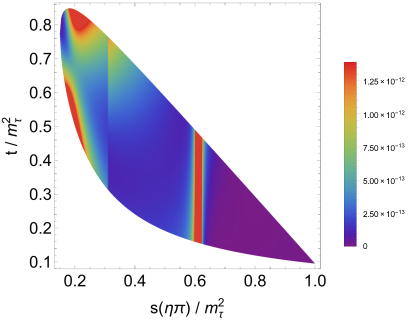
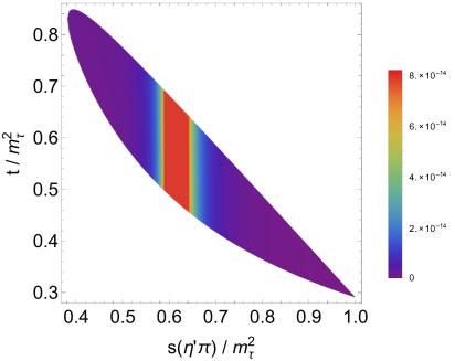
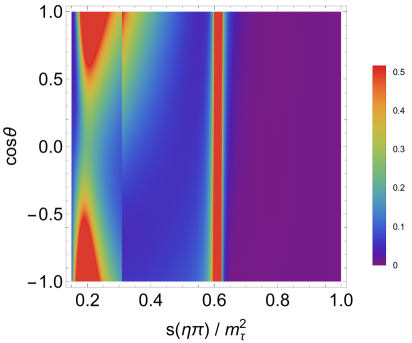
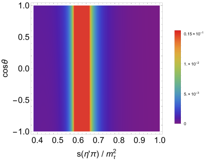
Figure 1: Dalitz plot distribution $\overline{|{\cal M}|^{2}}_{00}$ in the SM, eq. (22): the $\eta\pi$ ($\eta^{\prime}\pi$) case is shown in the left (right) column. The figures in the second row show the double differential decay distribution in the $(s,\cos\theta)$ variables according to eq. (24) normalized to the tau width, for both decay channels. The Mandelstam variables, $s$ and $t$, are normalized to $M_{\tau}^{2}$.

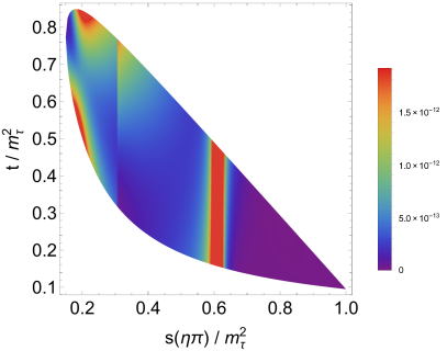
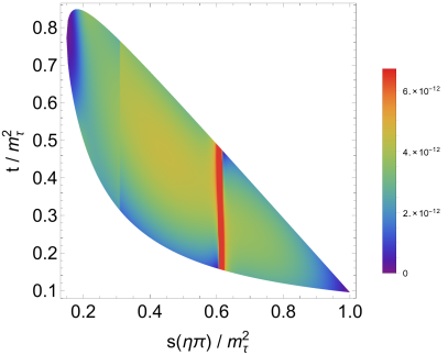
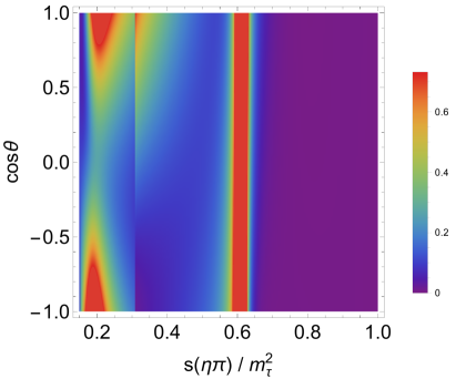
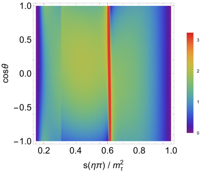
Figure 2: Dalitz plot distribution for $\tau^{-}\to\pi^{-}\eta\nu_{\tau}$ decays: left-hand side corresponds to $(\widehat{\epsilon}_{S}=0.002,\widehat{\epsilon}_{T}=0)$, while the figures in the right-hand side are obtained with the choice $(\widehat{\epsilon}_{S}=0,\widehat{\epsilon}_{T}=0.3)$. The figures in the first row correspond to eq. (22). Figures in the lower row corresponding to eq. (24) are normalized to $\Gamma_{\tau}$. The Mandelstam variables, $s$ and $t$, are normalized to $M_{\tau}^{2}$.

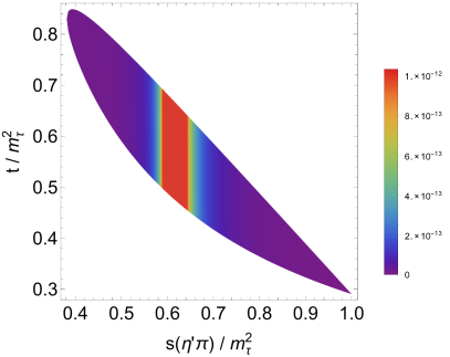
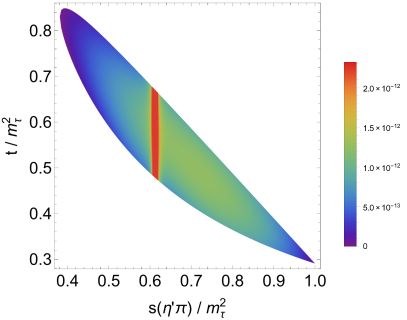
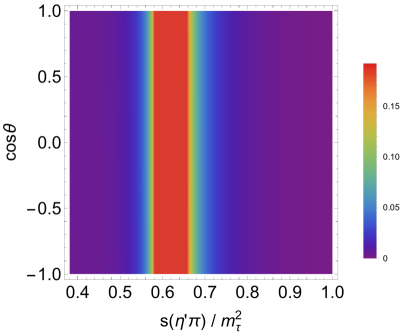
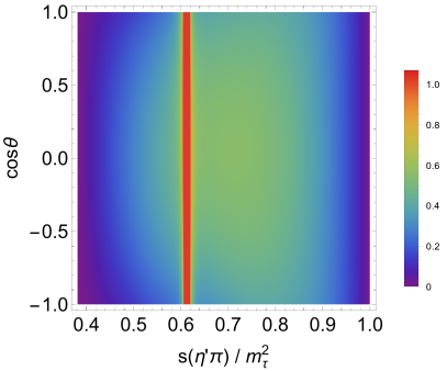
Figure 3: Dalitz plot distribution for $\tau^{-}\to\pi^{-}\eta^{\prime}\nu_{\tau}$ decays: figures in the left correspond to $(\widehat{\epsilon}_{S}=0.006,\widehat{\epsilon}_{T}=0)$, while those in the right side are obtained with the choice $(\widehat{\epsilon}_{S}=0,\widehat{\epsilon}_{T}=10)$. The figures in the first row correspond to eq. (22). The figures in the lower row to corresponding to eq. (24) are normalized to the tau width. The Mandelstam variables, $s$ and $t$, are normalized to $M_{\tau}^{2}$.

V.2 Angular distribution

The hadronic mass and angular distributions of decay products are also modified by the effects of New Physics contributions and can offer a different sensitivity to the scalar and tensor interactions. For this purpose it becomes convenient to set in the rest frame of the hadronic system defined by $\vec{p}_{\pi}+\vec{p}_{\eta^{(\prime)}}=\vec{p}_{\tau}-\vec{p}_{\nu_{\tau}}=0$. In this frame, the pion and tau lepton energies are given by $E_{\tau}=(s+M_{\tau}^{2})/2\sqrt{s}$ and $E_{\pi}=(s+m_{\pi}^{2}-m_{\eta^{(\prime)}}^{2})/2\sqrt{s}$. The angle $\theta$ between the three-momenta of the pion and tau lepton is related to the invariant $t$ variable by $t=m_{\tau}^{2}+m_{\pi}^{2}-2E_{\tau}E_{\pi}+2|\vec{p}_{\pi}||\vec{p}_{\tau}|\cos\theta$, where $|\vec{p}_{\pi}|=\sqrt{E_{\pi}^{2}-m_{\pi}^{2}}$ and $|\vec{p}_{\tau}|=\sqrt{E_{\tau}^{2}-m_{\tau}^{2}}$.

The decay distribution in the $(s,\cos\theta)$ variables in the framework of the most general effective interactions is given by

$$\frac{d^{2}\Gamma}{d\sqrt{s}d\cos\theta} = \frac{G_{F}^{2}|V_{ud}|^{2}S_{EW}}{128\pi^{3}m_{\tau}}(1+\epsilon_{L}+\epsilon_{R})^{2}\left(\frac{m^{2}_{\tau}}{s}-1\right)^{2}|\vec{p}_{\pi}|\left\{(c_{S}\Delta^{\rm QCD}_{K^{0}K^{+}})^{2}|{F}_{0}^{\pi^{-}\eta^{(\prime)}}(s)|^{2}\right.$$ (24)

$$\left.\times\left(1+\frac{s\widehat{\epsilon}_{S}}{m_{\tau}(m_{d}-m_{u})}\right)^{2}+16|\vec{p}_{\pi}|^{2}s^{2}\left|\frac{c_{V}}{2m_{\tau}}F_{+}^{\pi^{-}\eta^{(\prime)}}(s)-\widehat{\epsilon}_{T}F_{T}\right|^{2}\right.$$

$$\left.+4|\vec{p}_{\pi}|^{2}s\left(1-\frac{s}{m^{2}_{\tau}}\right)\left[c^{2}_{V}|F_{+}^{\pi^{-}\eta^{(\prime)}}(s)|^{2}+4\widehat{\epsilon}_{T}F^{2}_{T}s\right]\cos^{2}\theta+4c_{S}\Delta^{\rm QCD}_{K^{0}K^{+}}|\vec{p}_{\pi}|\sqrt{s}\cos\theta\right.$$

$$\left.\ \times\left(1+\frac{s\widehat{\epsilon}_{S}}{m_{\tau}(m_{d}-m_{u})}\right)\left[c_{V}{\rm Re}[F_{0}(s)F_{+}^{*}(s)]-2\frac{s}{m_{\tau}}\widehat{\epsilon_{T}}F_{T}{\rm Re}[F_{0}(s)]\right]\right\}\ .$$

When the effective couplings of new interactions are turned off, we recover the usual expressions for this observable in the SM Beldjoudi:1994hi . It is interesting to observe that no new angular dependencies appear owing to the presence of new interactions, although the coefficients of $\cos\theta$ terms get modified by terms that increase with the hadronic invariant mass $s$. In this respect, it is interesting to point out that the last term of eq. (24), which is linear in cos$\theta$, would allow to probe the relative phase between the scalar and vector contributions in the absence of new physics. We note that similar modifications to the angular and hadronic-mass distributions are expected for allowed $\tau^{-}\to(P_{1}P_{2})^{-}\nu_{\tau}$ decays, although the effects of scalar and tensor interactions should be very small in those cases.

Results obtained using eq.(24) are plotted in the second row of figure 1 for $\eta\pi^{-}$ ($\eta^{\prime}\pi^{-}$) in the left (right) panel for the SM case. In the second row of figures 2, 3 we plot the $(s,\cos\theta)$ distributions, which are defined from eq. (24), using the same representative values of $(\widehat{\epsilon}_{S},\widehat{\epsilon}_{T})$ parameters for every channel employed above.

In general, a comparison between figures 1, 2 and 3 shows that, remarkably, differences between SM and New Physics distributions can be obtained either using the $(s,t)$ or the $(s,$ cos$\theta)$ Dalitz plot analyses. Then, the experimentally cleanest of these will be more useful restricting non-standard interactions. If both are available, consistency checks can be done by comparing their respective data.

V.3 Decay rate

Integration upon the $t$ variable in eq. (20) gives the hadronic invariant mass distributions

$$\frac{d\Gamma}{ds} = \frac{G_{F}^{2}S_{EW}m_{\tau}^{3}\Big{|}V_{ud}F_{+}^{\pi^{-}\eta^{(\prime)}}(0)\Big{|}^{2}}{384\pi^{3}s}(1+\epsilon_{L}+\epsilon_{R})^{2}\left(1-\frac{s}{m_{\tau}^{2}}\right)^{2}\lambda^{1/2}\left({s,m_{\eta^{(\prime)}}}^{2},{m_{\pi}}^{2}\right)$$ (25)

$$\ \ \ \ \ \ \ \ \ \ \ \ \ \times\left[X_{VA}+\widehat{\epsilon}_{S}X_{S}+\widehat{\epsilon}_{T}X_{T}+\widehat{\epsilon}_{S}^{2}X_{S^{2}}+\widehat{\epsilon}_{T}^{2}X_{T^{2}}\right],\,$$

where

$$X_{VA} = \frac{1}{s^{2}}\left[3|\widetilde{F}_{0}^{\pi^{-}\eta^{(\prime)}}(s)|^{2}\Delta_{\pi^{-}\eta^{(\prime)}}^{2}+|\widetilde{F}_{+}^{\pi^{-}\eta^{(\prime)}}(s)|^{2}\lambda\left(s,{m_{\eta^{(\prime)}}}^{2},{m_{\pi}}^{2}\right)\left(1+\frac{2s}{m_{\tau}^{2}}\right)\right]\,,$$

$$X_{S} = \frac{6}{s~{}m_{\tau}}|\widetilde{F}_{0}^{\pi^{-}\eta^{(\prime)}}(s)|^{2}]\frac{\Delta_{\pi^{-}\eta^{(\prime)}}^{2}}{m_{d}-m_{u}}\,,$$

$$X_{T} = \frac{-6\sqrt{2}}{s~{}m_{\tau}}\frac{\rm{Re}[F_{+}(s)]F_{T}}{|F_{+}^{\pi^{-}\eta^{(\prime)}}(0)|^{2}}\lambda\left(s,{m_{\eta^{(\prime)}}}^{2},{m_{\pi}}^{2}\right)\,,$$

$$X_{S^{2}} = \frac{3}{m_{\tau}^{2}}|\widetilde{F}_{0}^{\pi^{-}\eta^{(\prime)}}(s))|^{2}\frac{\Delta_{\pi^{-}\eta^{(\prime)}}^{2}}{(m_{d}-m_{u})^{2}}\,,$$ (26)

$$X_{T^{2}} = \frac{4}{s}\frac{|{F_{T}}|^{2}}{|F_{+}(0)|^{2}}\left(1+\frac{s}{2m_{\tau}^{2}}\right)\lambda\left(s,{m_{\eta}^{(\prime)}}^{2},{m_{\pi}}^{2}\right)\,.$$

Notice that when $\epsilon_{L}=\epsilon_{R}=\widehat{\epsilon}_{S}=\widehat{\epsilon}_{T}=0$ we recover the SM result from Escribano:2016ntp . We also note that by using finiteness of the matrix element at the origin, and the fact that the form factors are normalized at the origin, we have Escribano:2016ntp

$$F_{+}^{\pi^{-}\eta^{(\prime)}}(0)=-\frac{c^{S}_{\pi^{-}\eta^{(\prime)}}}{c^{V}_{\pi^{-}\eta^{(\prime)}}}\frac{\Delta^{\rm QCD}_{K^{0}K^{+}}}{\Delta_{\pi^{-}\eta^{(\prime)}}}F_{0}^{\pi^{-}\eta^{(\prime)}}(0)\ ,$$ (27)

and

$$\widetilde{F}_{+,0}^{\pi^{-}\eta^{(\prime)}}(s)=\frac{F_{+,0}^{\pi^{-}\eta^{(\prime)}}(s)}{F_{+,0}^{\pi^{-}\eta^{(\prime)}}(0)}\ ,$$ (28)

which have been used to write eq. (25).

In figure 4 we plot the invariant mass distributions of the hadronic system for $\tau^{-}\to\pi^{-}\eta^{(\prime)}\nu_{\tau}$ decays. Noticeable differences are observed outside the resonance peak region ($M_{S}\sim 1.39$ GeV, Escribano:2016ntp ) when we allow for small departures from the SM. Again, the hadronic spectrum in both cases ($\pi\eta$ and $\pi\eta^{\prime}$) is able to distinguish New Physics contributions provided the scalar form factor contributions are known to a sufficient level of accuracy (we will quantify this statement in the next section). While the scalar non-standard interactions basically modify the spectrum (which essentially keeps its shape) as a global factor, tensor interactions act quite smoothly over the phase space (contrary to the scalar form factors, which are extremely peaked around $\sqrt{s}\sim 1.39$ GeV). This would soften the $\eta$ channel spectrum visibly (in logarithmic scale). Since the $\eta^{\prime}$ channel is so much dominated by the scalar form factor, the change in the spectrum would be even harder to be appreciated, and only a precise measurement of its tale could show a deviation from the SM case hinting to vector-tensor interference.

Figure 4: Left figure shows the $\eta\pi^{-}$ hadronic invariant mass distribution for the SM (solid line) and $\widehat{\epsilon_{s}}=0.004,\widehat{\epsilon_{T}}=0$ (dashed line), $\widehat{\epsilon_{s}}=0,\;\widehat{\epsilon_{T}}=0.6$ (dotted line). Right figure shows the $\eta^{\prime}\pi^{-}$ hadronic invariant mass distribution for the SM (solid line) and $\widehat{\epsilon_{s}}=0.005,\;\widehat{\epsilon_{T}}=0$ (dashed line), $\widehat{\epsilon_{s}}=0,\widehat{\epsilon_{T}}=10$ (dotted line). Units in axis are given in powers of GeV and the decay distributions are normalized to the tau decay width.

VI Results and discussion

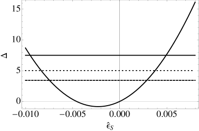
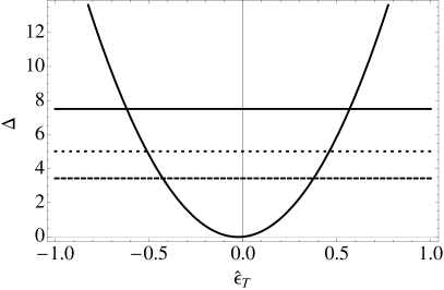
Figure 5: $\Delta$ as a function of $\widehat{\epsilon}_{S}$ (for $\widehat{\epsilon}_{T}=0)$ and $\widehat{\epsilon}_{T}$ (for $\widehat{\epsilon}_{S}=0)$ for $\tau^{-}\to\pi^{-}\eta\nu_{\tau}$ decays. Horizontal lines represent current values of $\Delta$ according to the upper limits on the branching fraction obtained by Babar (dotted line), $<9.9\times 10^{-5}$, $95\%$ CL delAmoSanchez:2010pc , Belle (dashed line), $<7.3\times 10^{-5}$, $90\%$ CL Hayasaka:2009zz and CLEO (solid line), $<1.4\times 10^{-4}$, $95\%$ CL Bartelt:1996iv .

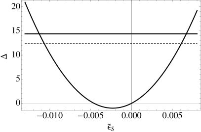
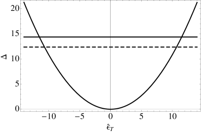
Figure 6: $\Delta$ as a function of $\widehat{\epsilon}_{S}$ (for $\widehat{\epsilon}_{T}=0)$ and $\widehat{\epsilon}_{T}$ (for $\widehat{\epsilon}_{S}=0)$ for $\tau^{-}\to\pi^{-}\eta^{\prime}\nu_{\tau}$ decays. Horizontal lines represent current values of $\Delta$ according to the upper limits on the branching fraction obtained by Babar (solid line), $<7.2\cdot 10^{-6}$, $95\%$ CL Aubert:2008nj and Belle (dashed line), $<4.6\cdot 10^{-6}$, $90\%$ CL Hayasaka:2009zz .

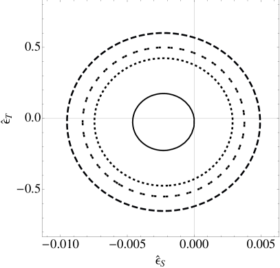
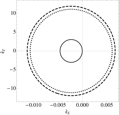
Figure 7: Left figure shows constraints on scalar and tensor couplings obtained from $\Delta(\tau^{-}\to\eta\pi^{-}\nu_{\tau})$ values using current experimental upper limits on branching fractions. The solid line represents $\Delta=0$, the dotted line is the Belle 90%CL limit, the doubly dotted line is the BaBar 95%CL limit and the dashed line is the CLEO 95%CL limit. In the right side we have contours of constant $\Delta(\tau^{-}\to\eta^{\prime}\pi^{-}\nu_{\tau})$ in the $\widehat{\epsilon}_{S}-\widehat{\epsilon}_{T}$ plane. The inner solid circle is the SM prediction, $\Delta=0$, the dotted line is the BaBar 95%CL limit and the dashed line is the Belle 90%CL limit.

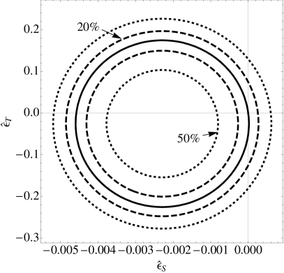
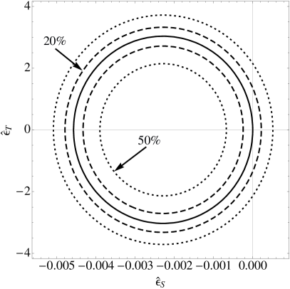
Figure 8: The thick solid line in the middle shows the contour for the SM Branching Ratio of $\tau^{-}\to\pi^{-}\eta^{(\prime)}\nu_{\tau}$. In the hypothetical case of this value being measured by Belle-II with 50%(band bounded with dotted lines) and 20%(band bounded with dashed lines) precision, some nonzero allowed range of values for $\widehat{\epsilon}_{S},\widehat{\epsilon}_{T}$ can be determined. In the left-hand side we have the case of $\tau^{-}\to\pi^{-}\eta\nu_{\tau}$, while on the right $\tau^{-}\to\pi^{-}\eta^{\prime}\nu_{\tau}$ is shown.

Equation (25) can be integrated to obtain the total decay rate of the $\tau^{-}\to\pi^{-}\eta^{(\prime)}\nu_{\tau}$ decays, using the expressions for the form factors discussed in Ref. Escribano:2016ntp and in Section IV. Since the total decay rate depends upon several effective couplings, we can explore how New physics effects inducing scalar and tensor interactions can be constrained by measurements of the branching fractions. For this purpose, we compare the decay rate ($\Gamma$) for $\tau^{-}\to\pi^{-}\eta^{(\prime)}\nu_{\tau}$ including all the interactions with respect to the one ($\Gamma^{0}$) obtained by neglecting $\widehat{\epsilon}_{S}$ and $\widehat{\epsilon}_{T}$ couplings. Integrating eq. (25) we get the shift produced by new physics contributions as follows

$$\Delta\equiv\frac{\Gamma-\Gamma^{0}}{\Gamma^{0}}=\alpha\widehat{\epsilon}_{S}+\beta\widehat{\epsilon}_{T}+\gamma\widehat{\epsilon}_{S}^{2}+\delta\widehat{\epsilon}_{T}^{2}\,.$$ (29)

Clearly, $\Delta=0$ when we have only vector current contributions to the decay amplitude. The numerical values of the coefficients are: $\alpha\sim(7\cdot 10^{2},9\cdot 10^{2}),~{}\beta\sim(1.1,-8\cdot 10^{-4}),~{}\gamma\sim(1.6\cdot 10^{5},1.9\cdot 10^{5})$ and $\delta\sim(21,0.1)$ where the first (second) value refers to $\pi\eta\;(\pi\eta^{\prime})$ channel. Easy-to-estimate uncertainties on these values are given by the corresponding errors of $\epsilon_{\pi\eta^{(\prime)}}$, given the quadratic dependence of observables on these mixing coefficients. For the most interesting case of $\alpha^{\pi\eta}$, this yields the range $\left[300,800\right]$, approximately.

Eq. (29) is a quadratic function of the effective scalar and tensor couplings that can be used to explore the sensitivity of $\tau^{-}\to\pi^{-}\eta^{(\prime)}\nu_{\tau}$ decays to the effects of New Physics. This can be achieved in two different ways. Firstly, we can represent the constraint on scalar (tensor) couplings obtained from the current upper limits on $\Gamma$ by assuming $\widehat{\epsilon}_{T}=0$ (respectively, $\widehat{\epsilon}_{S}=0)$. This is shown in figure 5 where we represent with horizontal lines the current experimental upper limits on $\Delta$ and eq. (29) for $\tau^{-}\to\pi^{-}\eta\nu_{\tau}$ decays. According to this procedure, we get the constraint $-0.008\leq\widehat{\epsilon}_{S}\leq 0.004$ which corresponds to the BaBar’s upper limit assuming $\widehat{\epsilon}_{T}=0$, left-hand side of figure 5. Constraints on tensor interactions are weaker: $|\widehat{\epsilon}_{T}|\leq 0.4$, assuming $\widehat{\epsilon}_{S}=0$ and BaBar’s upper limit, right-hand side of figure 5. Similar conclusions can be obtained for limits on the scalar coupling in the case of $\tau^{-}\to\pi^{-}\eta^{\prime}\nu_{\tau}$ decays, see figures 6. In this case $-0.011\leq\widehat{\epsilon}_{S}\leq 0.007$. It can be noticed that much looser limits are obtained for the tensor coupling in this case, $|\widehat{\epsilon}_{T}|\leq 11$.

Secondly, constraints on scalar and tensor interactions can be set simultaneously from a comparison of experimental upper limits and eq. (29). This is represented in figures 7, for the case of $\tau^{-}\to\pi^{-}\eta^{(\prime)}\nu_{\tau}$ decays. Clearly, the limits on the scalar and tensor couplings get slightly relaxed in this case with respect to the ones obtained when one of the couplings is assumed to vanish. These constraints can be largely improved at Belle II as it is shown in figures 8, where we compare the limits that can be set on the $(\widehat{\epsilon}_{S},\widehat{\epsilon}_{T})$ plane by assuming that the branching ratio of $\tau^{-}\to\pi^{-}\eta^{(\prime)}\nu_{\tau}$ can be measured with 50% and 20% accuracy. Left (right)-hand side of figures 8 shows the sensitivity on the scalar and tensor couplings that can be obtained from improved measurements of the $\tau^{-}\to\pi^{-}\eta\nu_{\tau}(\tau^{-}\to\pi^{-}\eta^{\prime}\nu_{\tau})$ branching fraction.

Table 1 summarizes the constraints on the scalar and tensor couplings that can be derived from the current upper limits on the branching ratios of $\tau^{-}\to\pi^{-}\eta^{(\prime)}\nu_{\tau}$ decays. We also display the constraints that can be obtained from forthcoming measurements of the branching fraction of these decays at Belle II experiment, by assuming a 20% accuracy .

$\Delta$	$\widehat{\epsilon}_{S}(\widehat{\epsilon}_{T}=0)$	$\widehat{\epsilon}_{T}(\widehat{\epsilon}_{S}=0)$	$\widehat{\epsilon}_{S}$	$\widehat{\epsilon}_{T}$
$\pi\eta$
Babar	$[-8.3,3.9]\cdot 10^{-3}$	[-0.43,0.39]	$[-0.83,0.37]\cdot 10^{-2}$	[-0.55,0.50]
Belle	$[-7.7,2.9]\cdot 10^{-3}$	[-0.51,0.47]	$[-0.75,0.29]\cdot 10^{-2}$	[-0.48,0.43]
CLEO	$[-9.5,5.0]\cdot 10^{-3}$	[-0.62,0.57]	$[-0.95,0.49]\cdot 10^{-2}$	[-0.66,0.60]
Belle II	$([-4.8,2.0]\cdot 10^{-3}$	[-0.12,0.08]	$[-4.9,-4.3]\cdot 10^{-3}\bigcup$	$[-0.20,-0.25]\bigcup$
			$[-2.6,3.0]\cdot 10^{-4}$	[0.15,0.20]
$\pi\eta^{\prime}$
Babar	$[-1.13,0.68]\cdot 10^{-2}$	$|\widehat{\epsilon}_{T}|<$11.4	$[-1.13,0.67]\cdot 10^{-2}$	[-11.9,11.9]
Belle	$[-1.07,0.60]\cdot 10^{-2}$	$|\widehat{\epsilon}_{T}|<$10.6	$[-1.06,0.61]\cdot 10^{-2}$	[-11.0,11.0]
Belle II	$[-4.8,2.3]\cdot 10^{-3}$	[-1.35,1.41]	$[-4.8,-4.3]\cdot 10^{-3}\bigcup$	$[-3.4,-2.7]\bigcup$
			$[-2.4,2.4]\cdot 10^{-4}$	$[2.7,3.3]$

Table 1: Constraints on the scalar and tensor couplings obtained from current upper limits on the branching fractions and hypothetical measurements with 20% accuracy at Belle II experiment.

At this point it is interesting to compare the limits in Table 1 to those obtained in Ref. Bhattacharya:2011qm (see also Cirigliano:2012ab ; Cirigliano:2013xha ; Gonzalez-Alonso:2013ura ). For this we need to assume lepton universality because our study involves the $\tau$ flavor, while theirs electron and muon flavors. However, given the smallness of possible lepton universality violations, this is enough for current precision. It is clear that $\tau^{-}\to\pi^{-}\eta^{(\prime)}\nu_{\tau}$ decays are not competitive restricting tensor interactions. Our upper limits (using present data) are at the level of $|\widehat{\epsilon_{T}}|\lesssim 0.5$ while the radiative pion decay reaches the $10^{-4}$ level through Dalitz plot analysis Mateu:2007tr ; Beldjoudi:1994hi ; Cirigliano:2012ab ; Cirigliano:2013xha ; Gonzalez-Alonso:2013ura ; Bychkov:2008ws . On the contrary, our bounds are very competitive in the case of scalar interactions, where we get (with current data) $-0.009<|\widehat{\epsilon_{S}}|<0.004$, while $0^{+}\to 0^{+}$ nuclear $\beta$ decays set limits (from the Fierz interference term) Hardy:2008gy at a few times $10^{-3}$ . The potential of a precise measurement of these decays at Belle-II is illustrated in the very stringent bounds on $\widehat{\epsilon_{S}}$ appearing in table 1. For this, however, it is crucial to improve our knowledge on the theoretical uncertainty of the scalar contribution . Being quite conservative, we have re-calculated these constraints assuming that the scalar contribution to observables in the $\eta$ channel can be a factor seven smaller than quoted in Escribano:2016ntp (like, for instance in Orsay’s group prediction Orsay ) and this results in increasing the upper bound on $|\widehat{\epsilon_{S}}|$ one order of magnitude. Before results of Belle-II searches on these tau decays become available, more precise measurements of meson-meson scattering would be of enormous help in reducing the errors of the dominant scalar form factors, allowing thus the derivation of sharp limits on non-standard scalar interactions, as put forward in this article.

VII Conclusions

The rare $\tau^{-}\to\pi^{-}\eta^{(\prime)}\nu_{\tau}$ decays, which are suppressed by G-parity in the Standard Model, can receive important contributions of New Physics. We have studied these decays in the framework of the most general effective field theory which incorporate dimension-six operators and assumes left-handed neutrinos. We have found that the Dalitz plot, hadronic invariant mass distribution and branching fraction are sensitive to the effects of scalar and tensor interactions and offer complementary information to the ones obtained from other low-energy processes.

These decays will probably be observed for the first time at the Belle II experiment. The different observables studied in this paper will be very useful to characterize the underlying dynamics of these decays. Our study indicates that these observables will be able to set very strong constraints on scalar interactions, or to set limits that are very competitive with other low-energy processes. To the best of our knowledge, this is the first study aiming to disentangle SCC from G-parity violation in sensitive observables of tau lepton decays.

References

• (1) T. D. Lee and C. N. Yang, Nuovo Cim.  10, 749 (1956).
• (2) C. Leroy and J. Pestieau, Phys. Lett.  72B, 398 (1978).
• (3) S. Weinberg, Phys. Rev.  112, 1375 (1958).
• (4) G. C. Branco, P. M. Ferreira, L. Lavoura, M. N. Rebelo, M. Sher and J. P. Silva, Phys. Rept.  516, 1 (2012)
• (5) M. Jung, A. Pich and P. Tuzón, JHEP 1011, 003 (2010).
• (6) D. Becirevic, S. Fajfer, N. Kosnik and O. Sumensari, Phys. Rev. D 94, 115021 (2016).
• (7) N. Severijns, M. Beck and O. Naviliat-Cuncic, Rev. Mod. Phys.  78 (2006) 991.
• (8) S. Triambak et al., Phys. Rev. C 95 (2017) , 035501 Addendum: [Phys. Rev. C 95 (2017), 049901].
• (9) Y. Meurice, Phys. Rev. D 36, 2780 (1987); A. Bramon, S. Narison and A. Pich, Phys. Lett. B 196 (1987) 543; A. Pich, Phys. Lett. B 196 (1987) 561; J. L. Díaz-Cruz and G. López Castro, Mod. Phys. Lett. A 6, 1605 (1991); S. Nussinov and A. Soffer, Phys. Rev. D 78, 033006 (2008), Phys. Rev. D 80, 033010 (2009); N. Paver and Riazuddin, Phys. Rev. D 82, 057301 (2010), Phys. Rev. D 84, 017302 (2011); M. K. Volkov and D. G. Kostunin, Phys. Rev. D 86, 013005 (2012);
• (10) H. Neufeld and H. Rupertsberger, Z. Phys. C 68, 91 (1995).
• (11) S. Descotes-Genon and B. Moussallam, Eur. Phys. J. C 74 (2014) 2946.
• (12) R. Escribano, S. Gonzàlez-Solís and P. Roig, Phys. Rev. D 94, 034008 (2016).
• (13) A. Guevara, G. López-Castro and P. Roig, Phys. Rev. D 95 (2017), 054015.
• (14) G. Hernández-Tomé, G. López-Castro and P. Roig, arXiv:1707.03037 [hep-ph]. To be published in Phys. Rev. D.
• (15) P. del Amo Sanchez et al. [BaBar Collaboration], Phys. Rev. D 83, 032002 (2011).
• (16) K. Hayasaka [Belle Collaboration], PoS EPS -HEP2009, 374 (2009).
• (17) J. E. Bartelt et al. [CLEO Collaboration], Phys. Rev. Lett.  76, 4119 (1996).
• (18) B. Aubert et al. [BaBar Collaboration], Phys. Rev. D 77 (2008) 112002.
• (19) T. Bergfeld et al. [CLEO Collaboration], Phys. Rev. Lett.  79 (1997) 2406.
• (20) T. Abe et al. [Belle-II Collaboration], arXiv:1011.0352 [physics.ins-det].
• (21) Belle-II Physics Book, Belle-II Collaboration and B2TIP-Community, to be published in Progress of Theoretical and Experimental Physics.
• (22) W. Buchmuller and D. Wyler, Nucl. Phys. B 268 (1986) 621.
• (23) B. Grzadkowski, M. Iskrzynski, M. Misiak and J. Rosiek, JHEP 1010 (2010) 085.
• (24) T. Bhattacharya, V. Cirigliano, S. D. Cohen, A. Filipuzzi, M. González-Alonso, M. L. Graesser, R. Gupta and H. W. Lin, Phys. Rev. D 85, 054512 (2012).
• (25) V. Cirigliano, J. Jenkins and M. González-Alonso, Nucl. Phys. B 830, 95 (2010).
• (26) H. M. Chang, M. González-Alonso and J. Martín Camalich, Phys. Rev. Lett.  114 (2015) no.16, 161802.
• (27) M. González-Alonso and J. Martín Camalich, JHEP 1612 (2016) 052.
• (28) M. González-Alonso and J. Martín Camalich, arXiv:1606.06037 [hep-ph].
• (29) A. Sirlin, Rev. Mod. Phys. 50, 573 (1978); Nucl. Phys. B71, 29 (1974); W. J. Marciano and A. Sirlin, Phys. Rev. Lett. 61, 1815 (1988), ibid. 71, 3629 (1993); W. J. Marciano and A. Sirlin, Phys. Rev. Lett. 56, 22 (1986); A. Sirlin, Nucl. Phys. B196, 83 (1982); J. Erler, Rev. Mex. Fis.  50, 200 (2004).
• (30) A. Pich, Rept. Prog. Phys.  58 (1995) 563; G. Ecker, Prog. Part. Nucl. Phys.  35 (1995) 1.
• (31) S. Aoki et al., Eur. Phys. J. C 77 (2017) no.2, 112.
• (32) S. Weinberg, Physica A 96 (1979) 327.
• (33) J. Gasser and H. Leutwyler, Annals Phys.  158 (1984) 142.
• (34) J. Gasser and H. Leutwyler, Nucl. Phys. B 250 (1985) 465.
• (35) G. Colangelo, G. Isidori and J. Portolés, Phys. Lett. B 470, 134 (1999).
• (36) C. Patrignani et al. [Particle Data Group], Chin. Phys. C 40 (2016) no.10, 100001.
• (37) O. Catà and V. Mateu, Phys. Rev. D 77 (2008) 116009.
• (38) D. Becirevic, V. Lubicz, F. Mescia and C. Tarantino, JHEP 0305 (2003) 007.
• (39) V. M. Braun, T. Burch, C. Gattringer, M. Gockeler, G. Lacagnina, S. Schaefer and A. Schafer, Phys. Rev. D 68 (2003) 054501.
• (40) M. A. Donnellan et al., PoS LAT 2007 (2007) 369.
• (41) O. Catà and V. Mateu, JHEP 0709, 078 (2007).
• (42) H. Leutwyler, Nucl. Phys. Proc. Suppl.  64 (1998) 223; R. Kaiser and H. Leutwyler, In *Adelaide 1998, Nonperturbative methods in quantum field theory* 15-29; R. Kaiser and H. Leutwyler, Eur. Phys. J. C 17 (2000) 623.
• (43) J. Schechter, A. Subbaraman and H. Weigel, Phys. Rev. D 48 (1993) 339; T. Feldmann, P. Kroll and B. Stech, Phys. Rev. D 58 (1998) 114006; Phys. Lett. B 449 (1999) 339; T. Feldmann, Int. J. Mod. Phys. A 15 (2000) 159.
• (44) V. Mateu and J. Portolés, Eur. Phys. J. C 52, 325 (2007). O. Cata and V. Mateu, Phys. Rev. D 77, (2008) 116009.
• (45) L. Beldjoudi and T. N. Truong, Phys. Lett. B 351 (1995) 357.
• (46) V. Cirigliano, M. González-Alonso and M. L. Graesser, JHEP 1302 (2013) 046.
• (47) V. Cirigliano, S. Gardner and B. Holstein, Prog. Part. Nucl. Phys.  71 (2013) 93.
• (48) M. González-Alonso and J. Martín Camalich, Phys. Rev. Lett.  112 (2014), 042501.
• (49) M. Bychkov et al., Phys. Rev. Lett.  103 (2009) 051802.
• (50) J. C. Hardy and I. S. Towner, Phys. Rev. C 79 (2009) 055502.
• (51) M. B. Voloshin, Phys. Lett. B 283 (1992) 120.
• (52) P. Herczeg, Phys. Rev. D 49 (1994) 247.
• (53) B. A. Campbell and D. W. Maybury, Nucl. Phys. B 709 (2005) 419.
• (54) V. Cirigliano and I. Rosell, Phys. Rev. Lett.  99 (2007) 231801
• (55) J. A. Oller and E. Oset, Nucl. Phys. A 620 (1997) 438 Erratum: [Nucl. Phys. A 652 (1999) 407].
• (56) A. Furman and L. Lesniak, Phys. Lett. B 538 (2002) 266.
• (57) D. V. Bugg, Phys. Rev. D 78 (2008) 074023.
• (58) Z. H. Guo and J. A. Oller, Phys. Rev. D 84 (2011) 034005.
• (59) Z. H. Guo, J. A. Oller and J. Ruiz de Elvira, Phys. Rev. D 86 (2012) 054006.
• (60) Z. H. Guo, J. A. Oller and J. Ruiz de Elvira, Phys. Lett. B 712 (2012) 407.
• (61) C. Adolph et al. [COMPASS Collaboration], Phys. Lett. B 740 (2015) 303.
• (62) M. Albaladejo and B. Moussallam, Eur. Phys. J. C 75 (2015) no.10, 488.
• (63) C. Adolph et al. [COMPASS Collaboration], Phys. Rev. D 95 (2017) no.3, 032004.
• (64) J. J. Dudek et al. [Hadron Spectrum Collaboration], Phys. Rev. D 93 (2016) no.9, 094506.
• (65) Z. H. Guo, L. Liu, U. G. Meißner, J. A. Oller and A. Rusetsky, Phys. Rev. D 95 (2017) no.5, 054004.
• (66) M. Albaladejo and B. Moussallam, Eur. Phys. J. C 77 (2017) no.8, 508.