Abstract

We introduce a dynamic mechanism for the solution of analytically-tractable substructure in probabilistic programs, using conjugate priors and affine transformations to reduce variance in Monte Carlo estimators. For inference with Sequential Monte Carlo, this automatically yields improvements such as locally-optimal proposals and Rao–Blackwellization. The mechanism maintains a directed graph alongside the running program that evolves dynamically as operations are triggered upon it. Nodes of the graph represent random variables, edges the analytically-tractable relationships between them. Random variables remain in the graph for as long as possible, to be sampled only when they are used by the program in a way that cannot be resolved analytically. In the meantime, they are conditioned on as many observations as possible. We demonstrate the mechanism with a few pedagogical examples, as well as a linear-nonlinear state-space model with simulated data, and an epidemiological model with real data of a dengue outbreak in Micronesia. In all cases one or more variables are automatically marginalized out to significantly reduce variance in estimates of the marginal likelihood, in the final case facilitating a random-weight or pseudo-marginal-type importance sampler for parameter estimation. We have implemented the approach in Anglican and a new probabilistic programming language called Birch.

 

Delayed Sampling and Automatic Rao–Blackwellization of Probabilistic Programs

 

Lawrence M. Murray                        Daniel Lundén                        Jan Kudlicka Uppsala University                        KTH Royal Institute of Technology                        Uppsala University

David Broman                        Thomas B. Schön KTH Royal Institute of Technology                        Uppsala University

1 INTRODUCTION

Probabilistic programs extend graphical models with support for stochastic branches, in the form of conditionals, loops, and recursion. Because they are highly expressive, they pose a challenge in the design of appropriate inference algorithms. This work focuses on Sequential Monte Carlo (SMC) inference algorithms [4], extending an arc of research that includes probabilistic programming languages (PPLs) such as Venture [14], Anglican [26], Probabilistic C [18], WebPPL [8], Figaro [20], and Turing [7], as well as similarly-motivated software such as LibBi [16] and BiiPS [25].

The simplest SMC method, the bootstrap particle filter [9], requires only simulation—not pointwise evaluation—of the prior distribution. While widely applicable, it may be suboptimal with respect to Monte Carlo variance in situations where, in fact, pointwise evaluation is possible, so that other options are viable. One way of reducing Monte Carlo variance is to exploit analytical relationships between random variables, such as conjugate priors and affine transformations. Within SMC, this translates to improvements such as the locally-optimal proposal, variable elimination, and Rao–Blackwellization (see [5] for an overview). The present work seeks to automate such improvements for the user of a PPL.

Typically, a probabilistic program must be run in order to discover the relationships between random variables. Because of stochastic branches, different runs may discover different relationships, or even different random variables. While an equivalent graphical model might be constructed for any single run, it would constitute only partial observation. It may take many runs to observe the full model, if this is possible in finite time at all. We therefore seek a runtime mechanism for the solution of analytically-tractable substructure, rather than a compile-time mechanism of static analysis.

A general-purpose programming language can be augmented with some additional constructs, called checkpoints, to produce a PPL (see e.g. [26]). Two checkpoints are usual, denoted $\func{sample}$ and $\func{observe}$. The first suggests that a value for a random variable needs to be sampled, the second that a value for a random variable is given and needs to be conditioned upon. At these checkpoints, random behavior may occur in the otherwise-deterministic execution of the program, and intervention may be required by an inference algorithm to produce a correct result.

The simplest inference algorithm instantiates a random variable when first encountered at a $\func{sample}$ checkpoint, and updates a weight with the likelihood of a given value at an $\func{observe}$ checkpoint. This produces samples from the prior distribution, weighted by their likelihood under the observations. It corresponds to importance sampling with the posterior as the target and the prior as the proposal. A more sophisticated inference algorithm runs multiple instances of the program simultaneously, pausing after each $\func{observe}$ checkpoint to resample amongst executions. This corresponds to the bootstrap particle filter (see e.g. [26]).

These are forward methods, in the sense that checkpoints are executed in the order encountered, and sampling is myopic of future observations. The present work introduces a mechanism to change the order in which checkpoints are executed so that sampling can be informed by future observations, exploiting analytical relationships between random variables. This facilitates more sophisticated forward-backward methods, in the sense that information from future observations can be propagated backward through the program.

We refer to this new mechanism as delayed sampling. When a $\func{sample}$ checkpoint is reached, its execution is delayed. Instead, a new node representing the random variable is inserted into a graph that is maintained alongside the running program. This graph resembles a directed graphical model of those random variables encountered so far that are involved in analytically-tractable relationships. Each node of the graph is marginalized and conditioned by analytical means for as long as possible until, eventually, it must be instantiated for the program to continue execution. This occurs when the random variable is passed as an argument to a function for which no analytical overload is provided. It is at this last possible moment that sampling is executed and the random variable instantiated.

Operations on the graph are forward-backward. The forward pass is a filter, marginalizing each latent variable over its parents and conditioning on observations, in all cases analytically. The backward pass produces a joint sample. This has some similarity to belief propagation [19], but the backward passes differ: belief propagation typically obtains the marginal posterior distribution of each variable, not a joint sample. Furthermore, in delayed sampling the graph evolves dynamically as the program executes, and at any time represents only a fraction of the full model. This means that some heuristic decisions must be made without complete knowledge of the model structure.

For SMC, delayed sampling yields locally-optimal proposals, variable elimination, and Rao–Blackwellization, with some limitations, to be detailed later. At worst, it provides no benefit. There is little intrusion of the inference algorithm into modeling code, and possibly no intrusion with appropriate language support. This is important, as we consider the user experience and ergonomics of a PPL to be of primary importance.

Related work has considered analytical solutions to probabilistic programs. Where a full analytical solution is possible, it can be achieved via symbolic manipulations in Hakaru [23]. Where not, partial solutions using compile-time program transformations are considered in [17] to improve the acceptance rate of Metropolis–Hastings algorithms. This compile-time approach requires careful treatment of stochastic branches, and even then it may not be possible to propagate analytical solutions through them. Delayed sampling instead operates dynamically, at runtime. It handles stochastic branches without problems, but may introduce some additional execution overhead.

The paper is organized as follows. Section 2 introduces the delayed sampling mechanism. Section 3 provides a set of pedagogical examples and two empirical case studies. Section 4 discusses some limitations and future work. Supplementary material includes further details of the case studies and implementations.

2 METHODS

As a probabilistic program runs, its memory state evolves dynamically and stochastically over time, and can be considered a stochastic process. Let $t=1,2,\ldots$ index a sequence of checkpoints. These checkpoints may differ across program runs (this is one of the challenges of inference for probabilistic programs, see e.g. [27]). In contrast to the two-checkpoint $\func{sample}$-$\func{observe}$ formulation, we define three checkpoint types:

• $\func{assume}(X,p(\cdot))$ to initialize a random variable $X$ with prior distribution $p(\cdot)$,

• $\func{observe}(x,p(\cdot))$ to condition on a random variable $X$ with likelihood $p(\cdot)$ having some value $x$,

• $\func{value}(X)$ to realize a value for a random variable $X$ previously encountered at an $\func{assume}$ checkpoint.

We use the statistics convention that an uppercase character (e.g. $X$) denotes a random variable, while the corresponding lowercase character (e.g. $x$) denotes an instantiation of it.

An $\func{assume}$ checkpoint does not result in a random variable being sampled: its sampling is delayed until later. A $\func{value}$ checkpoint occurs the first time that a random variable, previously encountered by an $\func{assume}$, is used in such a way that its value is required. At this point it cannot be delayed any longer, and is sampled.

Denote the state of the running program at checkpoint $t$ by $X_{t}\in\mathbb{X}_{t}$. This can be interpreted as the current memory state of the program. Randomness is exogenous and represented by the random process $U_{t}\in\mathbb{U}_{t}$. This may be, for example, random entropy, a pseudorandom number sequence, or uniformly distributed quasirandom numbers.

The program is a sequence of functions $f_{t}$ that each maps a starting state $X_{t-1}=x_{t-1}$ and random input $U_{t}=u_{t}$ to an end state $X_{t}=x_{t}$, so that $x_{t}=f_{t}(x_{t-1},u_{t})$. Note that $f_{t}$ is a deterministic function given its arguments. It is not permitted that $f_{t}$ has any intrinsic randomness, only the extrinsic randomness provided by $U_{t}$.

The target distribution over $X_{t}$ is $\pi_{t}(\mathrm{d}x_{t})$, typically a Bayesian posterior. In general, the program cannot sample from this directly. Instead, it samples $x_{t}$ from some proposal distribution $q_{t}(\mathrm{d}x_{t})$, which in many cases is just the prior distribution $p_{t}(\mathrm{d}x_{t})$. Then, assuming that both $\pi_{t}$ and $q_{t}$ admit densities, it computes an associated importance weight $w_{t}\propto\pi_{t}(x_{t})/q_{t}(x_{t})$. Assuming $U_{t}$ is distributed according to $\xi_{t}(\mathrm{d}u_{t})$, we have

$$q_{t}(\mathrm{d}x_{t})=\int_{\mathbb{X}_{t-1}}\int_{\mathbb{U}_{t}}\delta_{f_{t}(x_{t-1},u_{t})}(\mathrm{d}x_{t})\xi_{t}(\mathrm{d}u_{t})q_{t-1}(\mathrm{d}x_{t-1}),$$

where $\delta$ is the Dirac measure. For brevity, we omit the subscript $t$ henceforth, and simply update the state for the next time, as though it is mutable.

2.1 Motivation

We are motivated by variance reduction in Monte Carlo estimators. Consider some functional $\varphi(X)$ of interest. We wish to compute expectations of the form:

$$\mathbb{E}_{\pi}[\varphi(X)] =\int_{\mathbb{X}}\varphi(x)\pi(\mathrm{d}x)=\int_{\mathbb{X}}\varphi(x)\frac{\pi(x)}{q(x)}q(\mathrm{d}x).$$

Self-normalized importance sampling estimates can be formed by running the program $N$ times and computing (where superscript $n$ indicates the $n$th program run):

$$\hat{\varphi}:=\sum_{n=1}^{N}\bar{w}^{n}\varphi(x^{n}),\quad\bar{w}^{n}=w^{n}\bigg{/}\sum_{n=1}^{N}w^{n}.$$

A classic aim is to reduce mean squared error:

$$\mathrm{MSE}(\hat{\varphi})=\mathbb{E}_{q}\left[\left(\hat{\varphi}-\mathbb{E}_{\pi}[\varphi(X)]\right)^{2}\right].$$

One technique to do so is Rao–Blackwellization (see e.g. [21, §4.2]). Assume that, amongst the state $X$, there is some variable $X_{v}$ which has been observed to have value $x_{v}$, some set of variables $X_{M}$ which can be marginalized out analytically, and some other set of variables $X_{R}$ which have been instantiated previously. The functional of interest is the incremental likelihood of $x_{v}$. An estimator would usually require instantiation of $X_{M}^{n}\sim p(\mathrm{d}x_{M}^{n}\mid x_{R}^{n})$ for $n=1,\ldots,N$, and computation of:

$$\hat{Z}:=\sum_{n=1}^{N}\bar{w}^{n}p(x_{v}\mid x_{M}^{n},x_{R}^{n}).$$

The Rao–Blackwellized estimator does not instantiate $X_{M}$, but rather marginalizes it out:

$$\hat{Z}_{RB}:=\sum_{n=1}^{N}\bar{w}^{n}\int p(x_{v}\mid x_{M}^{n},x_{R}^{n})p(\mathrm{d}x_{M}^{n}\mid x_{R}^{n}).$$

By the law of total variance, $\mathrm{var}(\hat{Z}_{RB})\leq\mathrm{var}(\hat{Z})$, and as $\hat{Z}$ and $\hat{Z}_{RB}$ are unbiased [3], $\mathrm{MSE}(\hat{Z}_{RB})\leq\mathrm{MSE}(\hat{Z})$.

This form of Rao–Blackwellization is local to each checkpoint. While $X_{M}$ is marginalized out, it may require instantiation at future checkpoints, and so it must also be possible to simulate $p(\mathrm{d}x_{M}\mid x_{v},x_{R})$.

2.2 Delayed sampling

Delayed sampling uses analytical relationships to reorder the execution of checkpoints and reduce variance. Each $\func{observe}$ is executed as early as possible, and the sampling associated with $\func{assume}$ is delayed for as long as possible, to be informed by observations in between.

Alongside the state $X$, we maintain a graph $G=(V,E)$. This is a directed graph consisting of a set of nodes $V$ and set of edges $E\subset V\times V$, where $(u,v)\in E$ indicates a directed edge from a parent node $u$ to a child node $v$. For $v\in V$, let $\mathrm{Pa}(v)=\{u\in V\mid(u,v)\in E\}$ denote its set of parents, and $\mathrm{Ch}(v)=\{u\in V\mid(v,u)\in E\}$ its set of children. Associated with each $v\in V$ is a random variable $X_{v}$ (part of the state, $X$) and prior probability distribution $p_{v}(\mathrm{d}x_{v}\mid x_{\mathrm{Pa}(v)})$, now using the subscript of $X$ to select that part of the state associated with a single node, or set of nodes. We partition $V$ into three disjoint sets according to three states. Let

• $I\subseteq V$ be the set of nodes in an initialized state,

• $M\subseteq V$ be the set of nodes in a marginalized state,

• $R\subseteq V$ be the set of nodes in a realized state.

At some checkpoint, the program would usually have instantiated all variables in $V$ with a simulated or observed value, whereas under delayed sampling only those in $R$ are instantiated, while those in $I\cup M$ are delayed.

We will restrict the graph $G$ to be a forest of zero or more disjoint trees, such that each node has at most one parent. This condition is easily ensured by construction: the implementation makes anything else impossible, i.e. only relationships between pairs of random variables are coded. There are some interesting relationships that cannot be represented as trees, such as a normal distribution with conjugate prior over both mean and variance, or multivariate normal distributions. We deal with these as special cases, collecting multiple nodes into single supernodes and implementing relationships between pairs of supernodes, much like the structure achieved by the junction tree algorithm [11].

The following invariants are preserved at all times:

1. If a node is in M then its parent is in M. (1)

2. A node has at most one child in M. (2)

These imply that the nodes of $M$ form marginalized paths: one in each of the disjoint trees of $G$, from the root node to a node (possibly itself) in the same tree. We will refer to the unique such path in each tree as its $M$-path. The node at the start of the $M$-path is a root node, while the node at the end is referred to as a terminal node. Terminal nodes have a special place in the algorithms below, and are denoted by the set $T$.

By the invariants, each $v\in M\setminus T$ has a child $u\in M$; let $\mathrm{Fo}(v)$ denote the entire subtree with this child $u$ as its root (the forward set). Otherwise let $\mathrm{Fo}(v)$ be the empty set. The graph $G$ then encodes the distribution

$$\left(\prod_{v\in I}q_{v}(\mathrm{d}x_{v}\mid x_{\mathrm{Pa}(v)})\right)\left(\prod_{v\in M\setminus T}q_{v}(\mathrm{d}x_{v}\mid x_{R\setminus\mathrm{Fo}(v)})\right)\times$$

$$\quad\left(\prod_{v\in T}q_{v}(\mathrm{d}x_{v}\mid x_{R})\right),$$ (3)

where $q_{v}$ equals the prior for nodes in $I$, some updated distribution for nodes in $M$, and all nodes in $R$ are instantiated. The distribution suggests why terminals (in the set $T$) are important: they are the nodes informed by all instantiated random variables up to the current point in the program, and can be immediately instantiated themselves. Other nodes in $M$ await information to be propagated backward from their forward set before they, too, can be instantiated.

When the program reaches a checkpoint, it triggers operations on the graph (details follow):

• For $\func{assume}(X_{v},p(\cdot)$), call $\proc{Initialize}(v,p(\cdot))$, which inserts a new node $v$ into the graph.

• For $\func{observe}(x_{v},p(\cdot))$, call $\proc{Initialize}(v,p(\cdot))$, then $\proc{Graft}(v)$, which turns $v$ into a terminal node, then $\proc{Observe}(v)$, which assigns the observed value to $v$ and updates its parent by conditioning.

• For $\func{value}(X_{v})$, call $\proc{Graft}(v)$, then $\proc{Sample}(v)$, which samples a value for $v$.

Figure 1 provides pseudocode for all operations; Figure 2 illustrates their combination. Operations are of two types: local and recursive. Local operations modify a single node and possibly its parent:

• $\proc{Initialize}(v,p(\cdot))$ inserts a new node $v$ into the graph. If $v$ requires a parent, $u$ (implied by $p(\cdot)$ having a conditional form, i.e. $p(\mathrm{d}x_{v}\mid x_{u})$ not $p(\mathrm{d}x_{v}$)), then $v$ is put in $I$ and the edge $(u,v)$ inserted. Otherwise, it is a root node and is put in $M$, with no edges inserted.

• $\proc{Marginalize}(v)$, where $v$ is the child of a terminal node, moves $v$ from $I$ to $M$ and updates its distribution by marginalizing over its parent.

• $\proc{Sample}(v)$ or $\proc{Observe}(v)$, where $v$ is a terminal node, assigns a value to the associated random variable by either sampling or observing, moves $v$ from $M$ to $R$, and updates the distribution of its parent node by conditioning. Both $\proc{Sample}(v)$ and $\proc{Observe}(v)$ use an auxiliary function $\proc{Realize}(v)$ for their common operations.

As shown in the pseudocode, these local operations have strict preconditions that limit their use to only a subset of the nodes of the graph, e.g. only terminal nodes may be sampled or observed. As long as these preconditions are satisfied, the invariants (1) and (2) are maintained, and the graph $G$ encodes the representation (3). This is straightforward to check.

The recursive operations realign the $M$-path to establish the preconditions for any given node, so that local operations may be applied to it. These have side effects, in that other nodes may be modified to achieve the realignment. The key recursive operation is $\proc{Graft}$, which combines local operations to extend the $M$-path to a given node, making it a terminal node. Internally, $\proc{Graft}$ may call another recursive operation, $\proc{Prune}$, to shorten the existing $M$-path by realizing one or more variables.

$\proc{Initialize}(v,p(\cdot))$ if $p$ includes a parent node, $u$ $I\leftarrow I\cup\{v\}$ $E\leftarrow E\cup\{(u,v)\}$ $q_{v}(\mathrm{d}x_{v})\leftarrow p(\mathrm{d}x_{v}\mid x_{u})$ else $M\leftarrow M\cup\{v\}$ $q_{v}(\mathrm{d}x_{v})\leftarrow p(\mathrm{d}x_{v})$

$\proc{Marginalize}(v)$ assert $v\in I$ and $v$ has a parent $u\in T$ $q_{v}(\mathrm{d}x_{v})\leftarrow\int_{\mathbb{X}_{u}}p(\mathrm{d}x_{v}\mid x_{u})q_{u}(\mathrm{d}x_{u})$ $I\leftarrow I\setminus\{v\}$ $M\leftarrow M\cup\{v\}$

$\proc{Sample}(v)$ assert $v\in T$ draw $x_{v}\sim q_{v}(\mathrm{d}x_{v})$ $\proc{Realize}(v)$

$\proc{Observe}(v)$ assert $v\in T$ $w\leftarrow q_{v}(x_{v})w$ $\proc{Realize}(v)$

$\proc{Realize}(v)$ assert $v\in T$ $M\leftarrow M\setminus\{v\}$ $R\leftarrow R\cup\{v\}$ if $v$ has a parent $u$ condition parent $q_{u}(\mathrm{d}x_{u})\leftarrow\frac{p(x_{v}\mid x_{u})q_{u}(\mathrm{d}x_{u})}{\int_{\mathbb{X}_{u}}p(x_{v}\mid x^{\prime}_{u})q_{u}(\mathrm{d}x^{\prime}_{u})}$ $E\leftarrow E\setminus\{(u,v)\}$ for $u\in\mathrm{Ch}(v)$ new roots from children $\proc{Marginalize}(u)$ $E\leftarrow E\setminus\{(v,u)\}$

$\proc{Graft}(v)$ if $v\in M$ if $v$ has a child $u\in M$ $\proc{Prune}(u)$ else $\proc{Graft}(u)$ where $u$ is the parent of $v$ $\proc{Marginalize}(v)$ assert $v\in T$

$\proc{Prune}(v)$ assert $v\in M$ if $v$ has a child $u\in M$ $\proc{Prune}(u)$ $\proc{Sample}(v)$

Figure 1: Operations on the graph. The left arrow ($\leftarrow$) denotes assignment. Assigning to a distribution is interpreted as updating its hyperparameters.

Figure 2: Demonstration of the $M$-path and operations on the graph. On the left, the $M$-path reaches from the root node, $a$, to the terminal node, $c$, marked in bold lines. The $\proc{Graft}$ operation is called for $d$. This requires a realignment of the $M$-path around $b$, pruning the previous $M$-path at $c$, then extending it through to $d$. The stack trace of operations is in the center, and the final state on the right. Descendants of $c$ that were not on the $M$-path are now the roots of separate, disjoint trees.

Program	Checkpoint	Local operations	Commentary
x ~ N(0,1);	$\func{assume}(X)$	$\proc{Initialize}(X)$	Named delay_triplet in supplementary material.
y ~ N(x,1);	$\func{assume}(Y)$	$\proc{Initialize}(Y)$
z ~ N(y,1);	$\func{observe}(z)$	$\proc{Initialize}(Z)$
		$\proc{Marginalize}(Y)$	No $\proc{Marginalize}(X)$ is necessary: $X$, as a root node, is initialized in the marginalized state.
		$\proc{Marginalize}(Z)$
		$\proc{Observe}(z)$
print(x);	$\func{value}(X)$	$\proc{Sample}(Y)$	Samples $Y\sim p(\mathrm{d}y\mid z)$.
		$\proc{Sample}(X)$	Samples $X\sim p(\mathrm{d}x\mid y,z)$.
print(y);			A value $Y=y$ is already known.
x ~ N(0,1);	$\func{assume}(X)$	$\proc{Initialize}(X)$	Named delay_iid in supplementary material. It encodes multiple i.i.d. observations with a conjugate prior distribution over their mean.
for (t in 1..T) {
y[t] ~ N(x,1);	$\func{observe}(y_{t})$	$\proc{Initialize}(y_{t})$
		$\proc{Marginalize}(y_{t})$
		$\proc{Observe}(y_{t})$
}
print(x);	$\func{value}(X)$	$\proc{Sample}(X)$	Samples $X\sim p(\mathrm{d}x\mid y_{1},\ldots,y_{T})$.
x ~ Bernoulli(p);	$\func{assume}(X)$	$\proc{Initialize}(X)$	Named delay_spike_and_slab in supplementary material. It encodes a spike-and-slab prior [15] often used in Bayesian linear regression.
if (x) {	$\func{value}(X)$	$\proc{Sample}(X)$
y ~ N(0,1);	$\func{assume}(Y)$	$\proc{Initialize}(Y)$
} else {
y <- 0;			Used as a regular variable, no graph operations are triggered.
}			$Y$ is marginalized or realized as some $Y=y$ by the end, according to the stochastic branch.
x[1] ~ N(0,1);	$\func{assume}(X_{1})$	$\proc{Initialize}(X_{1})$	Named delay_kalman in supplementary material. It encodes a linear-Gaussian state-space model, for which delayed sampling yields a forward Kalman filter and backward simulation.
y[1] ~ N(x[1],1);	$\func{observe}(y_{1})$	$\proc{Initialize}(y_{1})$
		$\proc{Marginalize}(y_{1})$
		$\proc{Observe}(y_{1})$
for (t in 2..T) {			After each $t$th iteration of this loop, the distribution $p(\mathrm{d}x_{t}\mid y_{1},\ldots,y_{t})$ is obtained; the behavior corresponds to a Kalman filter.
x[t] ~ N(a*x[t-1],1);	$\func{assume}(X_{t})$	$\proc{Initialize}(X_{t})$
y[t] ~ N(x[t],1);	$\func{observe}(y_{t})$	$\proc{Initialize}(y_{t})$
		$\proc{Marginalize}(X_{t})$
		$\proc{Marginalize}(y_{t})$
		$\proc{Observe}(y_{t})$
}
print(x[1]);	$\func{value}(X_{1})$	$\proc{Sample}(X_{T})$	Samples $X_{T}\sim p(\mathrm{d}x_{T}\mid y_{1},\ldots,y_{T})$.
		$\ldots$	Recursively samples $X_{t}\sim p(\mathrm{d}x_{t}\mid x_{t+1},y_{1},\ldots,y_{t})$ and computes $p(\mathrm{d}x_{t-1}\mid x_{t},y_{1},\ldots,y_{t-1})$.
		$\proc{Sample}(X_{1})$	Samples $X_{1}\sim p(\mathrm{d}x_{1}\mid x_{2},y_{1})$.

Table 1: Pedagogical examples of delayed sampling applied to four probabilistic programs, showing the programs themselves (first column), the checkpoints reached as they execute linearly from top to bottom (second column), the sequence of local operations that these trigger on the graph (third column), and commentary (fourth column). The programs use a Birch-like syntax. Random variables with given values (from earlier assignment) are annotated by underlining. The function print is assumed to accept real-valued arguments only, so may trigger a $\func{value}$ checkpoint when used.

3 EXAMPLES

We have implemented delayed sampling in Anglican (see also [13]) and a new PPL called Birch. Details are given in Appendices C and D.

Table 1 provides pedagogical examples using a Birch-like syntax, showing the sequence of checkpoints and graph operations triggered as some simple programs execute. They show how delayed sampling behaves through programming structures such as conditionals and loops, including stochastic branches.

In addition, we provide two case studies where delayed sampling improves inference, firstly a linear-nonlinear state-space model with simulated data, secondly a vector-borne disease model with real data from an outbreak of dengue virus in Micronesia. We use a simple random-weight or pseudo-marginal-type importance sampling algorithm for both of these examples:

1. Run SMC on the probabilistic program with delayed sampling enabled, producing $N$ number of samples $x^{1},\ldots,x^{N}$ with associated weights $w^{1},\ldots,w^{N}$ and a marginal likelihood estimate $\hat{Z}$.

2. Draw $a\in\{1,\ldots,N\}$ from the categorical distribution defined by $P(a)=w^{a}/\sum_{n=1}^{N}w^{n}$.

3. Output $x^{a}$ with weight $\hat{Z}$.

This produces one sample with associated weight, but may be repeated as many times as necessary—in parallel, even—to produce an importance sample as large as desired. The success of the approach depends on the variance of $\hat{Z}$. This variance can be reduced by marginalizing out one or more variables (recall Section 2.1). This is what delayed sampling achieves, and so we compare the variance of $\hat{Z}$ with delayed sampling enabled and disabled. When disabled, the SMC algorithm is simply a bootstrap particle filter. When enabled, it yields a Rao–Blackwellized particle filter. Where parameters are involved (as in the second case study), the diversity of parameter values depletes through the resampling step of SMC. This has motivated more sophisticated methods for parameter estimation such as particle Markov chain Monte Carlo methods [1], also applied to probabilistic programs [28]. Particle Gibbs is an obvious candidate here. We find, however, that the reduction in variance afforded by marginalizing out one or more variables with delayed sampling is sufficient to enable the above importance sampling algorithm for the two case studies here.

3.1 Linear-nonlinear state-space model

The first example is that of a mixed linear-nonlinear state-space model. For this model, delayed sampling yields a particle filter with locally-optimal proposal and Rao–Blackwellization.

The model is given by [12] and repeated in Appendix A. It consists of both nonlinear and linear-Gaussian state variables, as well as nonlinear and linear-Gaussian observations. Parameters are fixed. Ideally, the linear-Gaussian substructure is solved analytically (e.g. using a Kalman filter), leaving only the nonlinear substructure to sample (e.g. using a particle filter). The Rao–Blackwellized particle filter, also known as the marginalized particle filter, was designed to achieve precisely this [2, 22].

Delayed sampling automatically yields this method for this model, as long as analytical relationships between multivariate Gaussian distributions are encoded. In Birch these are implemented as supernodes: single nodes in the graph that contain multiple random variables. While the relationships between individual variables in a multivariate Gaussian have, in general, directed acyclic graph structure, their implementation as supernodes maintains the required tree structure.

The model is run for 100 time steps to simulate data. It is run again with SMC, conditioning on this data. For various numbers of particles, it is run 100 times to estimate $\hat{Z}$, with delayed sampling enabled and disabled. Figure 3 (left) plots the distribution of these estimates. Clearly, with delayed sampling enabled, fewer particles are needed to achieve comparable variance in the log-likelihood estimate.

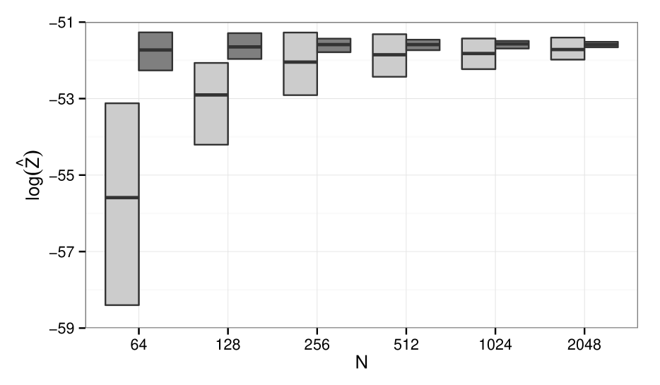
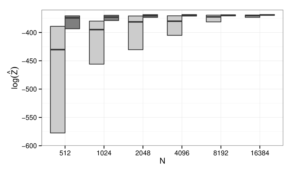
Figure 3: Distribution of the marginal log-likelihood estimate ($\log\hat{Z}$) for different numbers of particles ($N$) over 100 runs for (left) the linear-nonlinear state-space model, and (right) the vector-borne disease model, with (light gray) delayed sampling disabled, corresponding to a bootstrap particle filter, and (dark gray) delayed sampling enabled, corresponding to a Rao–Blackwellized particle filter. All runs use systematic resampling [10] when effective sample size falls below 0.7$N$. Boxes indicate the interquartile range, midline the median. In both cases, significantly fewer particles are required to achieve comparable variance when delayed sampling is enabled.

3.2 Vector-borne disease model

The second example is an epidemiological case study of an outbreak of dengue virus: a mosquito-borne tropical disease with an estimated 50-100 million cases and 10000 deaths worldwide each year [24]. It is based on the study in [6], which jointly models two outbreaks of dengue virus and one of Zika virus in two separate locations (and populations) in Micronesia. Presented here is a simpler study limited to one of those outbreaks, specifically that of dengue on the Yap Main Islands in 2011. The data used consists of 172 observations of reported cases, on a daily basis during the main outbreak, and on a weekly basis before and after.

The model consists of two components, representing the human and mosquito populations, coupled via cross-infection. Each population is further divided into subpopulations of susceptible, exposed, infectious and recovered individuals. At each time step a binomial transfer occurs between subpopulations, parameterized with conjugate beta priors. Details are in Appendix B.

The task is both parameter and state estimation. For this model, delayed sampling produces a Rao–Blackwellized particle filter where parameters, rather than state variables, are marginalized out. While the state variables are sampled immediately, the parameters are maintained in a marginalized state, conditioned on the samples of these state variables. This is a consequence of conjugacy between the beta priors on parameters and the binomial likelihoods of the state variables (as pseudo-observations).

For various numbers of particles, SMC is run 100 times to estimate $\hat{Z}$, with delayed sampling enabled and disabled. Figure 3 (right) plots the distribution of these estimates. Clearly, with delayed sampling enabled, fewer particles are needed to achieve comparable variance in the log-likelihood estimate. Some posterior results are given in Appendix B.

4 DISCUSSION AND CONCLUSION

Table 1 demonstrates how delayed sampling operates through typical program structures such as conditionals and loops, including stochastic branches as encountered in probabilistic programs. Figure 3 demonstrates the potential gains. These are particularly encouraging given that the mechanism is mostly automatic.

Some limitations are worth noting. The graph of analytically-tractable relationships must be a forest of disjoint trees. It is unclear whether this is a significant limitation in practice, but support for more general structures may be desirable. It is worth emphasizing that this relates to the structure of analytically-tractable relationships and the ability of the mechanism to utilize them, not to the structure of the model as a whole. At present, for more general structures, some opportunities for variance reduction are missed. One remedy is to encode supernodes, as for the multivariate Gaussian distributions in Section 3.1.

Delayed sampling potentially reorders the sampling associated with $\func{assume}$ checkpoints, and the interleaving of this amongst $\func{observe}$ checkpoints, but does not reorder the execution of $\func{observe}$ checkpoints. There is an opportunity cost to this. Consider the final example in Table 1: move the observations $y_{1},\ldots,y_{T}$ into a second loop that traverses time backward from $T$ to $1$. Delayed sampling now draws each $x_{t}$ from $p(\mathrm{d}x_{t}\mid x_{t+1},y_{t})$, not $p(\mathrm{d}x_{t}\mid x_{t+1},y_{1},\ldots,y_{t})$. This is suboptimal but not incorrect: whatever the distribution, importance weights correct for its discrepancy from the target. It is again unclear whether this is a significant limitation in practice; examples seem contrived and easily fixed by reordering code.

While delayed sampling may reduce the number of samples required for comparable variance, it does require additional computation per sample. For univariate relationships (e.g. beta-binomial, gamma-Poisson), this overhead is constant and—we conjecture—likely worthwhile for any fixed computational budget. For multivariate relationships the overhead is more complex and may not be worthwhile (e.g. multivariate Gaussian conjugacies require matrix inversions that are $\mathcal{O}(N^{3})$ in the number of dimensions). A thorough empirical comparison is beyond the scope of this article.

Finally, while the focus of this work is SMC, delayed sampling may be useful in other contexts. With undirected graphical models, for example, delayed sampling may produce a collapsed Gibbs sampler. This is left to future work.

Supplementary material

Appendix A details the linear-nonlinear state-space model, and Appendix B the vector-borne disease model. Appendix C details the Anglican implementation, and Appendix D the Birch implementation. Code is included for the pedagogical examples in both Anglican and Birch, and for the empirical case studies, along with data sets, in Birch only.

Appendix A Details of the linear-nonlinear state-space model

The full model is described in [12]. The state model contains both nonlinear ($X_{t}^{n}$) and linear-Gaussian ($X_{t}^{l}$) state variables, and is given by:

$$X_{0}^{n} \sim\mathcal{N}(0,1)$$

$$X_{t}^{n} \sim\mathcal{N}(\arctan x_{t-1}^{n}+Bx_{t-1}^{l},0.01)$$

$$X_{0}^{l} \sim\mathcal{N}(0,I_{3\times 3})$$

$$X_{t}^{l} \sim\mathcal{N}(Ax_{t-1}^{l},0.01I_{3\times 3}).$$

The observation model contains both nonlinear ($Y_{t}^{n}$) and linear-Gaussian ($Y_{t}^{l}$) observations, and is given by:

$$Y_{t}^{n} \sim\mathcal{N}\left(0.1(x_{t}^{n})^{2}\mathrm{sgn}(x_{t}^{n}),0.1\right)$$

$$Y_{t}^{l} \sim\mathcal{N}(Cx_{t}^{l},0.1I_{3\times 3}).$$

Parameters are fixed as follows:

$$A =\begin{pmatrix}1&0.3&0\\ 0&0.92&-0.3\\ 0&0.3&0.92\end{pmatrix}$$

$$B =\begin{pmatrix}1&0&0\end{pmatrix}$$

$$C =\begin{pmatrix}1&-1&1\end{pmatrix}.$$

Appendix B Details of the vector-borne disease model

The process model is a discrete-time and discrete-state stochastic model based on the continuous-time and continuous-state deterministic mean-field approximation used in [6]. It consists of two SEIR (susceptible, exposed, infectious, recovered) compartmental models, one for the human population, the other for the mosquito population, coupled via cross-infection terms. Each component consists of state variables giving population counts in each of the four compartments: $s$ (susceptible), $e$ (exposed), $i$ (infectious), and $r$ (recovered), along with a total population $n$ that maintains the identity $n=s+e+i+r$, and parameters $\nu$ (birth probability), $\mu$ (death probability), $\lambda$ (transmission probability), $\delta$ (infectious probability), and $\gamma$ (recovery probability). A susceptible human may become infected when bitten by an infectious mosquito, while a susceptible mosquito may become infected when biting an infectious human.

We use superscript $h$ to denote state variables and parameters associated with the human component, and superscript $m$ to denote those associated with the mosquito component. For state variables, subscripts index time in days.

B.1 Initial condition model

For the setting of Yap Main Islands in 2011, the following initial conditions are prescribed:

$$n_{0}^{h} =7370 n_{0}^{m} =10^{u}n_{0}^{h}$$

$$s_{0}^{h} =n_{0}^{h}-e_{0}^{h}-i_{0}^{h}-r_{0}^{h} s_{0}^{m} =n_{0}^{m}$$

$$e_{0}^{h} \sim\mathrm{Poisson}(10) e_{0}^{m} =0$$

$$i_{0}^{h}-1 \sim\mathrm{Poisson}(10) i_{0}^{m} =0$$

$$r_{0}^{h} \sim\mathrm{Binomial}(n_{1}^{h},6/100) r_{0}^{m} =0,$$

with $u\sim\mathcal{U}(-1,2)$.

B.2 Transition model

The model transitions in two steps. The first step is an exchange between compartments that preserves total population. Denoting with primes the intermediate state after this first step, we have:

$$s_{t}^{h\prime} =s_{t-1}^{h}-\oplus e_{t}^{h} s_{t}^{m\prime} =s_{t-1}^{m}-\oplus e_{t}^{m}$$

$$e_{t}^{h\prime} =e_{t-1}^{h}+\oplus e_{t}^{h}-\oplus i_{t}^{h} e_{t}^{m\prime} =e_{t-1}^{m}+\oplus e_{t}^{m}-\oplus i_{t}^{m}$$

$$i_{t}^{h\prime} =i_{t-1}^{h}+\oplus i_{t}^{h}-\oplus r_{t}^{h} i_{t}^{m\prime} =i_{t-1}^{m}+\oplus i_{t}^{m}-\oplus r_{t}^{m}$$

$$r_{t}^{h\prime} =r_{t-1}^{h}+\oplus r_{t}^{h} r_{t}^{m\prime} =r_{t-1}^{m}+\oplus r_{t}^{m},$$

with the newly exposed, infectious, and recovered populations distributed as:

$$\oplus e_{t}^{h} \sim\mathrm{Binomial}(\tau_{t}^{h},\lambda^{h}) \oplus e_{t}^{m} \sim\mathrm{Binomial}(\tau_{t}^{m},\lambda^{m})$$

$$\oplus i_{t}^{h} \sim\mathrm{Binomial}(e_{t-1}^{h},\delta^{h}) \oplus i_{t}^{m} \sim\mathrm{Binomial}(e_{t-1}^{m},\delta^{m})$$

$$\oplus r_{t}^{h} \sim\mathrm{Binomial}(i_{t-1}^{h},\gamma^{h}) \oplus r_{t}^{m} \sim\mathrm{Binomial}(i_{t-1}^{m},\gamma^{m}),$$

for parameters $\lambda^{h}$, $\delta^{h}$, $\gamma^{h}$, $\lambda^{m}$, $\delta^{m}$, $\gamma^{m}$. The $\tau_{t}^{h}$ gives the number of susceptible humans bitten by at least one infectious mosquito, and $\tau_{t}^{m}$ the number of susceptible mosquitos that bite at least one infectious human:

$$\tau_{t}^{h} \sim\mathrm{Binomial}\left(s_{t-1}^{h},1-\exp(-i_{t-1}^{m}/n_{t-1}^{h})\right)$$ (4)

$$\tau_{t}^{m} \sim\mathrm{Binomial}\left(s_{t-1}^{m},1-\exp(-i_{t-1}^{h}/n_{t-1}^{h})\right).$$ (5)

These latter quantities are derived by assuming (a) a $\mathrm{Poisson}(n_{t}^{m})$ number of mosquito blood meals per day with these interactions uniformly distribution across both humans and mosquitos, (b) that a human is infected with probability $\lambda^{h}$ if interacting one or more times with an infectious mosquito, and (c) that a mosquito is infected with probability $\lambda^{m}$ if interacting one or more times with an infectious human. Note that the $n_{t-1}^{h}$ appearing in (4) is correct, although one may expect to see $n_{t-1}^{m}$ given the otherwise-symmetry of the equations of this model. In the derivation, $n_{t-1}^{m}$ also appears in the denominator of both (4) and (5), but cancels with the Poisson rate parameter for the number of blood meals, also given by $n_{t}^{m}$ as above.

The second step accounts for births and deaths:

$$s_{t}^{h} =s_{t}^{h\prime}-\ominus s_{t}^{h}+\oplus n_{t}^{h} s_{t}^{m} =s_{t}^{m\prime}-\ominus s_{t}^{m}+\oplus n_{t}^{m}$$

$$e_{t}^{h} =e_{t}^{h\prime}-\ominus e_{t}^{h} e_{t}^{m} =e_{t}^{m\prime}-\ominus e_{t}^{m}$$

$$i_{t}^{h} =i_{t}^{h\prime}-\ominus i_{t}^{h} i_{t}^{m} =i_{t}^{m\prime}-\ominus i_{t}^{m}$$

$$r_{t}^{h} =r_{t}^{h\prime}-\ominus r_{t}^{h} r_{t}^{m} =r_{t}^{m\prime}-\ominus r_{t}^{m},$$

with births distributed as

$$\oplus n_{t}^{h} \sim\mathrm{Binomial}(n_{t}^{h\prime},\nu^{h}) \oplus n_{t}^{m} \sim\mathrm{Binomial}(n_{t}^{m\prime},\nu^{m}),$$

with parameters $\nu^{h}$ and $\nu^{m}$, and deaths as

$$\ominus s_{t}^{h} \sim\mathrm{Binomial}(s_{t}^{h\prime},\mu^{h}) \ominus s_{t}^{m} \sim\mathrm{Binomial}(s_{t}^{m\prime},\mu^{m})$$

$$\ominus e_{t}^{h} \sim\mathrm{Binomial}(e_{t}^{h\prime},\mu^{h}) \ominus e_{t}^{m} \sim\mathrm{Binomial}(e_{t}^{m\prime},\mu^{m})$$

$$\ominus i_{t}^{h} \sim\mathrm{Binomial}(i_{t}^{h\prime},\mu^{h}) \ominus i_{t}^{m} \sim\mathrm{Binomial}(i_{t}^{m\prime},\mu^{m})$$

$$\ominus r_{t}^{h} \sim\mathrm{Binomial}(r_{t}^{h\prime},\mu^{h}) \ominus r_{t}^{m} \sim\mathrm{Binomial}(r_{t}^{m\prime},\mu^{m}),$$

with parameters $\mu^{h}$ and $\mu^{m}$.

B.3 Observation model

Observations are of the number of new infectious cases reported at health centers, aggregated over the time since the last such observation (this is daily during the peak time of the outbreak and weekly either side). For times $t\in\left\{1,\ldots,T\right\}$ where observations are available, the observation model is given by

$$y_{t}\sim\mathrm{Binomial}\left(\sum_{s=t-l_{t}+1}^{t}\oplus i_{s}^{h},\rho\right),$$

where $l_{t}$ (lag) indicates the number of days since the last observation. Significant under-reporting of cases is expected, reflected in the parameter $\rho$.

B.4 Parameter model

The following fixed values and priors are assigned to parameters, translating prior knowledge on rates in [6] to prior knowledge on probabilities here:

$$\nu_{h} =0 \nu_{m} =1/7$$

$$\mu_{h} =0 \mu_{m} =1/7$$

$$\lambda_{h} \sim\mathrm{Beta}(1,1) \lambda_{m} \sim\mathrm{Beta}(1,1)$$

$$\delta_{h} \sim\mathrm{Beta}\left(\frac{16}{11},\frac{28}{11}\right) \delta_{m} \sim\mathrm{Beta}\left(\frac{17}{13},\frac{35}{13}\right)$$

$$\gamma_{h} \sim\mathrm{Beta}\left(\frac{13}{9},\frac{23}{9}\right) \gamma_{m} =0.$$

Birth and death in the human population are assumed to be of minimal impact over the course of the outbreak, and so their rates are fixed to zero. The expected lifespan of a mosquito is one week, with birth and death rates fixed accordingly. Mosquitos do not recover before death.

Finally, the prior over the reporting probability is

$$\rho\sim\mathrm{Beta}(1,1).$$

B.5 Inference results

Inference is performed by drawing 10000 weighted samples, each time running SMC with 8192 particles. The effective sample size of these 10000 weighted samples is computed to be 2260. Some results are shown in Figure 4.

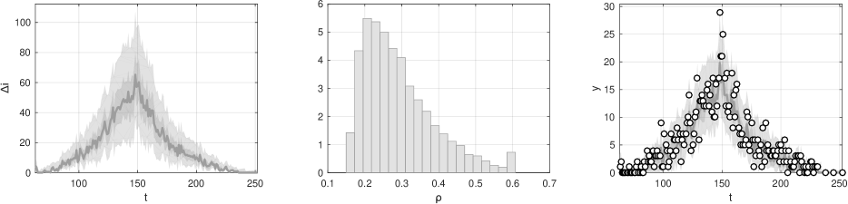
Figure 4: Posterior results for the vector-borne disease model example, (left) posterior distribution of newly infectious cases in humans over time, $\oplus i_{t}^{h}$, (middle) posterior distribution of the reporting probability parameter, $\rho$, and (right) posterior predictive distribution of the number of reported cases, $y$, overlaid with actual observations. In the left and right plots, the bold line gives the median, darker shaded region the 50% credibility interval, and lighter shaded region the 95% credibility interval.

Appendix C Anglican implementation

Anglican is a functional probabilistic programming language integrated with Clojure. Clojure, in turn, is a Lisp dialect which compiles to Java virtual machine bytecode, enabling reuse of the Java infrastructure. The Anglican compiler is built with Clojure macros, and compiles Anglican programs into continuation-passing-style Clojure code. This transformation enables inference algorithms to affect the control flow and record information at checkpoints. Manipulations are performed both on the continuations themselves and on the state, which is passed along as an argument in each continuation call.

For simplicity, delayed sampling is implemented entirely on top of the existing Anglican language, leaving the original language constructs and functionality untouched. A set of new keywords and functions are added for usage of delayed sampling: ds-<name>, ds-value, and ds-observe. The ds-value and ds-observe functions loosely correspond to the $\proc{Sample}$ and $\proc{Observe}$ operations in Section 2.2, but ds-value also includes functionality for retrieving values for already-sampled nodes. The set of ds-<name> functions correspond to the $\proc{Initialize}$ operations in Section 2.2, for various probability distributions, e.g. ds-normal. The delayed sampling graph is conveniently encoded in the already existing Anglican state.

As an example, consider the following line of code:

let [x (ds-normal mean sd)]

This binds x to a graph node which is normally distributed with mean mean and standard deviation sd. To subsequently introduce another normally distributed graph node with the node x as mean, one can write

let [y (ds-normal x sd’)]

passing the previous graph node x as a parameter. This will initialize a conjugate prior relationship between them. If y is then observed, x will be conditioned on the observed value of y.

Appendix D Birch implementation

Birch is a compiled, imperative, object-oriented, generic, and probabilistic programming language. The latter is its primary research concern. The Birch compiler uses C++ as a target language.

Delayed sampling has been implemented using the Birch type system. Special types are used when declaring variables to make them eligible for delayed sampling. For example, a variable that might ordinarily be declared to be of type Real may be declared to be of type Random<Real> to make it eligible for delayed sampling. The generic class Random implements the behavior required for delayed sampling, and is specialized into classes that encode distributions (e.g. Gaussian), then further into classes that encode distributions with analytical relationships to others (e.g. GaussianWithGaussianMean). The graph required for delayed sampling is formed implicitly through objects of these classes and their member attributes.

Birch supports implicit type conversion, compiling directly to the same feature in C++. These implicit conversions are used to automatically trigger the $\func{value}$ checkpoint, and are resolved at compile time. For example, a Random<Real> object may be passed to a function that requires a Real argument. An implicit conversion is used to trigger a $\func{value}$ checkpoint, realizing a value of type Real from the object of type Random<Real>. In this way, the programmer need not explicitly indicate $\func{value}$ checkpoints.

References

- Andrieu et al. [2010] C. Andrieu, A. Doucet, and R. Holenstein. Particle Markov chain Monte Carlo methods. Journal of the Royal Statistical Society B, 72:269–302, 2010. doi: 10.1111/j.1467-9868.2009.00736.x.
- Chen and Liu [2000] R. Chen and J. S. Liu. Mixture Kalman filters. Journal of the Royal Statistical Society B, 62:493–508, 2000.
- Del Moral [2004] P. Del Moral. Feynman-Kac Formulae: Genealogical and Interacting Particle Systems with Applications. Springer–Verlag, New York, 2004.
- Del Moral et al. [2006] P. Del Moral, A. Doucet, and A. Jasra. Sequential Monte Carlo samplers. Journal of the Royal Statistical Society B, 68:441–436, 2006. doi: 10.1111/j.1467-9868.2006.00553.x.
- Doucet and Johansen [2011] A. Doucet and A. M. Johansen. A tutorial on particle filtering and smoothing: fifteen years later, chapter 24, pages 656–704. Oxford University Press, 2011.
- Funk et al. [2016] S. Funk, A. J. Kucharski, A. Camacho, R. M. Eggo, L. Yakob, L. M. Murray, and W. J. Edmunds. Comparative analysis of dengue and Zika outbreaks reveals differences by setting and virus. PLOS Neglected Tropical Diseases, 10(12):1–16, 12 2016. doi: 10.1371/journal.pntd.0005173.
- Ge et al. [2016] H. Ge, A. Ścibior, K. Xu, and Z. Ghahramani. Turing: A fast imperative probabilistic programming language. Technical report, June 2016.
- Goodman and Stuhlmüller [2014] N. D. Goodman and A. Stuhlmüller. The design and implementation of probabilistic programming languages. http://dippl.org, 2014.
- Gordon et al. [1993] N. Gordon, D. Salmond, and A. Smith. Novel approach to nonlinear/non-Gaussian Bayesian state estimation. IEE Proceedings-F, 140:107–113, 1993. doi: 10.1049/ip-f-2.1993.0015.
- Kitagawa [1996] G. Kitagawa. Monte Carlo filter and smoother for non-Gaussian nonlinear state space models. Journal of Computational and Graphical Statistics, 5:1–25, 1996. doi: 10.2307/1390750.
- Lauritzen and Spiegelhalter [1988] S. L. Lauritzen and D. J. Spiegelhalter. Local computations with probabilities on graphical structures and their application to expert systems. Journal of the Royal Statistical Society B, 1988.
- Lindsten and Schön [2010] F. Lindsten and T. B. Schön. Identification of mixed linear/nonlinear state-space models. In 49th IEEE Conference on Decision and Control (CDC), pages 6377–6382, 2010.
- Lundén [2017] D. Lundén. Delayed sampling in the probabilistic programming language Anglican. Master’s thesis, KTH Royal Institute of Technology, School of Computer Science and Communication, 2017.
- Mansinghka et al. [2014] V. K. Mansinghka, D. Selsam, and Y. N. Perov. Venture: a higher-order probabilistic programming platform with programmable inference. arXiv abs/1404.0099, 2014.
- Mitchell and Beauchamp [1988] T. J. Mitchell and J. J. Beauchamp. Bayesian variable selection in linear regression. Journal of the American Statistical Association, 83:1023–1032, 1988. doi: 10.2307/2290129.
- Murray [2015] L. M. Murray. Bayesian state-space modelling on high-performance hardware using LibBi. Journal of Statistical Software, 67(10):1–36, 2015. doi: 10.18637/jss.v067.i10.
- Nori et al. [2014] A. Nori, C.-K. Hur, S. Rajamani, and S. Samuel. R2: An efficient MCMC sampler for probabilistic programs. AAAI Conference on Artificial Intelligence (AAAI), 2014.
- Paige and Wood [2014] B. Paige and F. Wood. A compilation target for probabilistic programming languages. 31st International Conference on Machine Learning (ICML), 2014.
- Pearl [1988] J. Pearl. Probabilistic Reasoning in Intelligent Systems: Networks of Plausible Inference. Morgan Kaufmann, 1988.
- Pfeffer [2016] A. Pfeffer. Practical Probabilistic Programming. Manning, 2016.
- Robert and Casella [2004] C. Robert and G. Casella. Monte Carlo Statistical Methods. Springer-Verlag New York, 2004. doi: 10.1007/978-1-4757-4145-2.
- Schön et al. [2005] T. Schön, F. Gustafsson, and P. Nordlund. Marginalized particle filters for mixed linear/nonlinear state-space models. IEEE Transactions on Signal Processing, 53:2279–2289, 2005. doi: 10.1214/193940307000000518.
- Shan and Ramsey [2017] C. Shan and N. Ramsey. Exact Bayesian inference by symbolic disintegration. 44th ACM SIGPLAN Symposium on Principles of Programming Languages (POPL), 2017.
- Stanaway et al. [2016] J. D. Stanaway, D. S. Shepard, E. A. Undurraga, Y. A. Halasa, L. E. Coffeng, O. J. Brady, S. I. Hay, N. Bedi, I. M. Bensenor, C. A. Castañeda Orjuela, T.-W. Chuang, K. B. Gibney, Z. A. Memish, A. Rafay, K. N. Ukwaja, N. Yonemoto, and C. J. L. Murray. The global burden of dengue: an analysis from the Global Burden of Disease Study 2013. The Lancet Infectious Diseases, 16(6):712–723, 2016. doi: 10.1016/s1473-3099(16)00026-8.
- Todeschini et al. [2014] A. Todeschini, F. Caron, M. Fuentes, P. Legrand, and P. Del Moral. Biips: Software for Bayesian inference with interacting particle systems. arXiv abs/1412.3779, 2014.
- Tolpin et al. [2016] D. Tolpin, J. van de Meent, H. Yang, and F. Wood. Design and implementation of probabilistic programming language Anglican. arXiv abs/1608.05263, 2016.
- Wingate et al. [2011] D. Wingate, A. Stuhlmueller, and N. Goodman. Lightweight implementations of probabilistic programming languages via transformational compilation. 14th International Conference on Artificial Intelligence and Statistics (AISTATS), pages 770–778, 2011.
- Wood et al. [2014] F. Wood, J. W. van de Meent, and V. Mansinghka. A new approach to probabilistic programming inference. Proceedings of the 17th International Conference on Artificial Intelligence and Statistics (AISTATS), 2014.