Integral Curvature Representation and Matching Algorithms
for Identification of Dolphins and Whales

Abstract

We address the problem of identifying individual cetaceans from images showing the trailing edge of their fins. Given the trailing edge from an unknown individual, we produce a ranking of known individuals from a database. The nicks and notches along the trailing edge define an individual’s unique signature. We define a representation based on integral curvature that is robust to changes in viewpoint and pose, and captures the pattern of nicks and notches in a local neighborhood at multiple scales. We explore two ranking methods that use this representation. The first uses a dynamic programming time-warping algorithm to align two representations, and interprets the alignment cost as a measure of similarity. This algorithm also exploits learned spatial weights to downweight matches from regions of unstable curvature. The second interprets the representation as a feature descriptor. Feature keypoints are defined at the local extrema of the representation. Descriptors for the set of known individuals are stored in a tree structure, which allows us to perform queries given the descriptors from an unknown trailing edge. We evaluate the top-$k$ accuracy on two real-world datasets to demonstrate the effectiveness of the curvature representation, achieving top-$1$ accuracy scores of approximately $95\%$ and $80\%$ for bottlenose dolphins and humpback whales, respectively.

1 Introduction

We address the problem of identifying individual cetaceans from images of their fins --- dorsal fins for bottlenose dolphins, and flukes for humpback whales. Fitting into the broad domain of contour-based recognition [15], the fin instance recognition problem is particularly challenging, as illustrated in Figures 1 and 2.

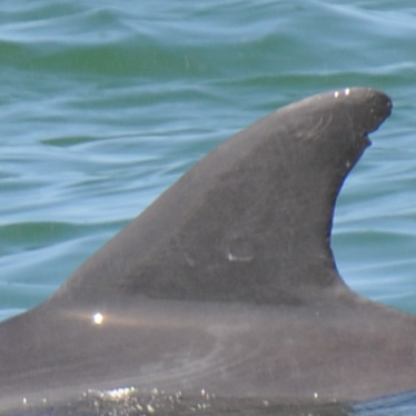
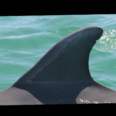
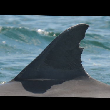
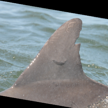
Figure 1: Example images of dorsal fins from the Bottlenose dolphin dataset. Although the fins in each row may appear similar, they are from distinct individuals. Note that the identifying information in each fin comes from one or two large markings. Compare this to the case for the Humpback dataset, where the identifying information is spread along the entire contour.

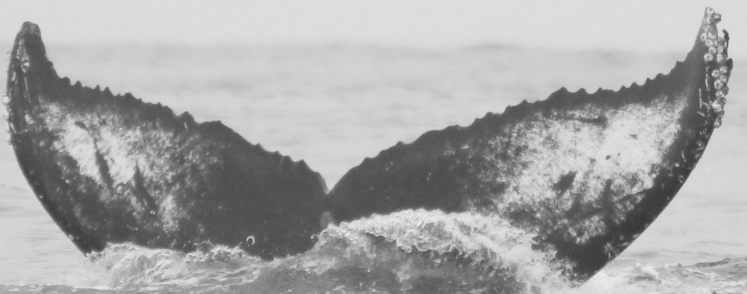
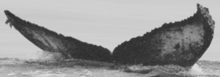
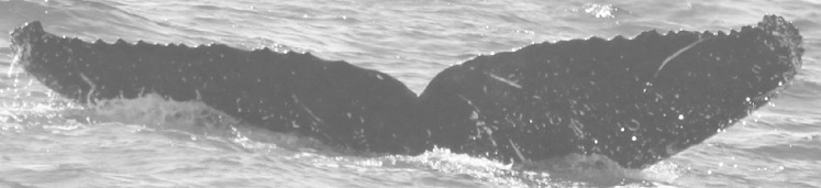
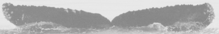
Figure 2: Example images of flukes from the Humpback whale dataset. The two upper images are from the same individual, while the two lower images are from distinct individuals. Note that, unlike for the Bottlenose dataset, the information necessary for identification is spread along the entire length of the fluke trailing edge.

Our hypothesis is that the information necessary to distinguish between the outlines of fins from distinct individuals is encoded in local measures of integral curvature [12]. Differential curvature measures have been applied to a variety of recognition problems, but these approaches are sensitive to noise [22]. Integral curvature, which produces more stable measurements, has been applied to category recognition problems like identifying leaf species [14].

In this paper, we propose novel combinations of integral curvature representation for extracted outline contours and two matching algorithms for identifying individuals. The first interprets the curvature representation as a sequence, and defines the similarity between two representations as the cost of warping one sequence onto the other. The second treats subsections of the representation as feature descriptors, and matches them using approximate nearest neighbors. Each takes a query image and produces a ranking of known individuals from a database. We also introduce a method for learning spatial weights that describe the relative importance of points along the trailing edge, which enables the matching algorithm to assign higher value to the most distinguishing areas of the fin contours.

In cetacean research, identifying individuals observed during a survey is a fundamental part of studying populations. Traditionally, techniques such as tagging or branding are used to make identification easier. Not only do these require specialized equipment and training, but they also tend to be invasive, requiring catch-and-release of wild animals. As a less invasive alternative, photo identification requires no direct contact with the animals. Instead, researchers use images of long-lasting markings, such as nicks, notches, or scars, to track individuals over time [28, 8].

Photo identification presents its own challenges. The images showing distinct individuals observed during a study need to be matched against a database containing images of known individuals. For large cetacean populations covering a large geographical area and monitored over a long time period, this can be very time-consuming when done using manual methods. Additionally, parts of the trailing edge required for identification are often occluded by water or viewpoint, requiring the use of multiple images per individual. Even when the trailing edge contours are consistently visible, direct matching between trailing edges from different images is problematic. Because the images are captured ‘‘in the wild’’, animals occur in a wide variety of poses and are photographed from varying viewpoints. Even for a small change in viewpoint, out-of-plane rotations can lead to difficulty in matching nicks and notches.

By presenting likely matches for a query individual to the user in order of similarity, manual identification may be substantially accelerated by reducing (on average) the number of individuals to compare per query.

1.1 Time-Warping Sequence Alignment

It is possible to treat the curvature representations of the trailing edges as vectors and compute their similarity using any vector norm. The start and endpoints of fins are ambiguous, and pose and viewpoint stretch some sections and foreshorten others, so we need to account for nicks and notches occurring at differing locations along the trailing edge. We use a dynamic programming time-warping algorithm [23] that computes the alignment cost of two representations. Rather than a one-to-one matching, as with a vector norm, this allows many points from one representation to match to one point in the other, and vice versa. This warps one representation onto the other, where the alignment cost is the sum of errors for local correspondences [12].

1.2 Descriptor Indexing

Considering that the nicks and notches used for identification are often sparsely distributed along the trailing edge, and that points in between offer little value for identification, it seems desirable to use only the former when performing an identification. To do this, we compute local extrema in the trailing edge representation, i.e., points corresponding to regions of high curvature in the original trailing edge, and use these as feature keypoints [11]. Between these keypoints, we extract feature descriptors, resample them to a fixed length, and normalize using the Euclidean norm. All individuals from the database are stored in a tree-like structure, after which the most likely candidate matches for a given trailing edge are computed using the local naive Bayes nearest neighbor classifier [19].

1.3 Contributions

The primary contributions of this work are that we (a) develop an integral curvature measure to represent trailing edge contours in such a way that the representation is robust to changes in viewpoint and pose that make direct comparison difficult, (b) propose integration of these measures with time-warping alignment and descriptor indexing algorithms as two approaches for ranking potential matches, (c) develop a learning algorithm to weight sections of the trailing edge contour, and (d) produce results using this representation and these algorithms on real-world datasets from active cetacea research groups to confirm their efficacy.

2 Related Work

The curvature computed at points along a contour is often used to represent shape information [20, 14, 6]. For differential curvature, this is defined as the change of the angle of the normal vector along the length of the contour [6]. This representation is sensitive to noise, however, and instead we use integral curvature. A fixed shape is placed at points along the contour, while measuring the area of the intersection of the shape with the contour [22]. Using integral curvature to capture shape information is a key part of the Leafsnap system [14], which classifies leaves by using curvature histograms at multiple scales as shape features. We briefly compare to Leafsnap in Section 5.

In terms of identifying dolphins from their dorsal fins, most notable is DARWIN [24]. The key idea behind DARWIN is to account for changes in viewpoint by computing a transformation between two fins to align them, and using the resulting sum of squared distances to define a similarity score [25]. As pointed out in [7], a fundamental problem with this approach is that fins from distinct individuals are unlikely to align correctly, with the result that similarity scores cannot be compared reliably to produce a ranking.

Another system, Finscan [9], frames the problem of comparing two dorsal fins as a string matching problem [1]. In this setting, they compute a low-level string representation of the trailing edge curvature. Because the curvature function defined in terms of derivatives is typically noisy, they refine this representation to a high-level string representation. To compute the similarity between two string representations, they use a linear time-warping algorithm.

In both DARWIN and Finscan, the extraction of the trailing edge is a semi-automatic, interactive process where the user manually corrects an initial estimate of the trailing edge. The size of our datasets, as well as our goal of scaling to real-world scenarios, makes comparison with these systems impractical. Instead, we design our representation and matching algorithms to be robust against the occasional inaccurate trailing edge extraction.

In [11], the authors propose a trailing edge indexing algorithm and apply it to great white sharks. After defining keypoints for feature extraction by convolving the contour with a Difference-of-Gaussian kernel, they explore the use of both the Difference-of-Gaussian norm and the descriptor from [2]. The descriptor indexing algorithm in our work is similar, except that we instead use the curvature representation as a feature descriptor.

A notable approach to the more general problem of ranking is the triplet network [10, 27], a natural extension of the Siamese network [26, 4]. A triplet network is a neural network that learns a useful representation by minimizing the distance between the representations of instances of the same class, while maximizing the distance between representations from different classes. One key advantage of this approach is that the representation does not need to be designed by hand, rather, it is learned from a large set of labeled training data. The resulting representation is then used to embed query instances into the same space, where a ranking may be computed. We briefly explored the use of triplet networks using the original trailing edge contours as well as the curvature representation, but found that our small datasets would lead to overfitting. Additionally, the parametric nature of these models makes it difficult to apply them to new datasets [29], whereas we confirm in Section 5.3 that our approach may be applied unchanged to an unseen dataset of the same species.

3 Datasets and Preprocessing

We use two real-world datasets provided by active research groups to evaluate our approach. The first dataset is provided by the Sarasota Dolphin Research Program and is illustrated in Figure 1. This dataset contains $10,\!713$ images representing $401$ distinct bottlenose dolphins (Tursiops truncatus). Researchers take photos of the dolphins encountered at a particular time and place, and the best images of each individual are separated into encounters. These images are cropped to the dorsal fin and added to the dataset. The second dataset is provided by the Cascadia Research Collective and shown in Figure 2. This dataset contains $7,\!173$ images representing $3,\!572$ humpback whales (Megaptera novaeangliae). Unlike the first dataset where each individual appears in multiple images per encounter, here each individual typically appears in only a single image per encounter.

Given an image, a fully-convolutional neural network (FCNN) [16] outputs the probability that each pixel is part of the trailing edge. Anchor points are computed, and a shortest-path algorithm selects pixels based on costs determined by a combination of the FCNN and image gradients. For dorsal fins, this includes a spatial transformer network [13] that transforms the image such that the fin is approximately perpendicular to the image plane.

4 Individual Identification

4.1 Curvature Representation

Given a trailing edge contour represented as an ordered set of coordinates, $\{(x_{1},y_{1}),(x_{2},y_{2}),\ldots,(x_{n},y_{n})\}$, we wish to represent this contour such that it is robust to changes in viewpoint and pose. For this we use an integral curvature measure that captures local shape information at each point along the trailing edge. For a given point $(x_{i},y_{i})$ that lies on the trailing edge, we place a circle of radius $r$ at the point and find all points on the trailing edge that lie within this circle, i.e., $\mathbf{p}_{i}=\{(x_{j},y_{j})\mid(x_{i}-x_{j})^{2}+(y_{i}-y_{j})^{2}\leq r^{2}\}$. To describe a point $(x_{i},y_{i})$ by its local curvature, we first orient the points $\mathbf{p}_{i}$ such that $\mathbf{p}_{i}(1)$ and $\mathbf{p}_{i}(n)$ lie on a horizontal line. The coordinates of the points in $\mathbf{p}_{i}$ are then clipped to the dimensions of an axis-aligned square with side length $2r$ centered at $(x_{i},y_{i})$. Using the bottom side of this square as the axis for the independent variable, we use trapezoidal integration to approximate the area under the curve defined by the discrete points $\mathbf{p}_{i}$. We define the curvature $c\in[0,1]$ at this point as the ratio of the area under the curve to the total area of the square, which implies that the curvature value for a straight line is $c=0.5$. See Figure 3 for an illustration. By computing this integral curvature measure at all points along the trailing edge, we obtain the curvature representation of the trailing edge for a single value of $r$. To control the extent to which we capture local and global information, we vary the radius of the circle placed at each point by choosing multiple values of $r$ (typically four). The result is a matrix $C$ of dimensions $m\times n$, where $m$ is the number of values of $r$ that we choose and $n$ is the number of points along the trailing edge. The scalar $C_{ij}\in[0,1]$ is the curvature value for the $i$th value of $r$ at the $j$th point along the trailing edge.

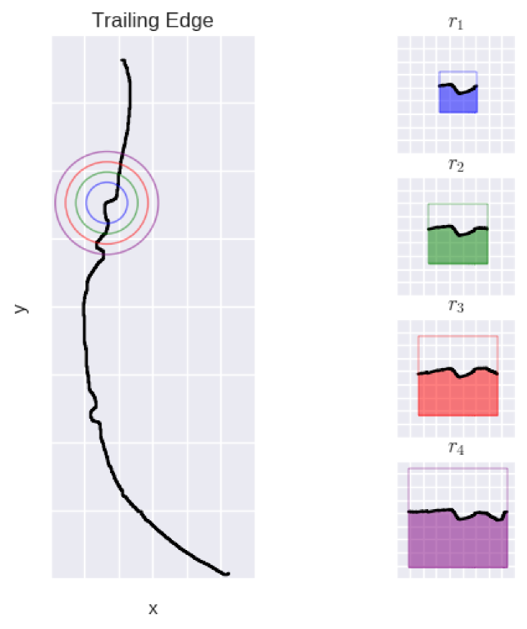
Figure 3: For a given point $(x_{j},y_{j})$, the curve segments lying inside circles of radii $r_{1},r_{2},\ldots,r_{m}$ (left) are transformed to be horizontal (right). The curvature at the point for a particular $r$ is then defined as the ratio of the area under the curve (shaded) to the area of a square of side length $2r$.

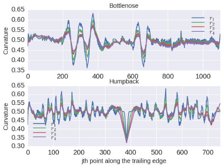
Figure 4: Curvature representation of a dorsal fin from the Bottlenose dataset (top) and fluke from the Humpback dataset (bottom) computed for four different values of $r$.

4.2 Ranking

We explore two types of methods that use the curvature representation defined in Section 4.1 to produce a ranking of known individuals given a query.

4.2.1 Sequence Alignment

Dynamic Time-Warping. The first method for comparing representations that we explore interprets the curvature representations as temporal sequences and computes an alignment cost between them [12, 23]. Given that the start and endpoints of the trailing edges are not only ambiguous, but also often under water, it is desirable to allow some degree of warping when computing correspondences. If we define $\mathbf{c}_{i}$ and $\mathbf{c}_{j}^{\prime}$ as the $i$th and $j$th columns (each a vector representing the curvature values at a point) of two curvature representations $C$ and $C^{\prime}$ of lengths $m$ and $m^{\prime}$, respectively, then the total alignment cost $c(m,m^{\prime})$ is defined recursively as

$$\mbox{}c(i,j) =d(\mathbf{c}_{i},\mathbf{c}_{j}^{\prime})$$

$$+\min\{c(i-1,j),c(i,j-1),c(i-1,j-1)\},$$ (1)

where $d$ defines the distance between two points based on their curvature values at multiple scales. It is possible to use a simple vector norm, such as $d(\mathbf{c}_{i},\mathbf{c}_{j}^{\prime})=||\mathbf{c}_{i}-\mathbf{c}_{j}^{\prime}||_{2}$.

Spatial Weights. The definition above, however, treats the contribution from correspondences along the entire length of the trailing edge as equal. We know that the end of the trailing edge is often underwater for dorsal fins, and the tips often cropped for flukes. Ideally, we would thus like corresponding points from these unstable regions to contribute less towards the total alignment cost.

To realize the above, we define a weight vector $\mathbf{w}$, where the elements $w_{1},w_{2},\ldots,w_{n}$ describe the relative importance of each point along the trailing edge. In doing so, we define a more meaningful distance function as

$$d(\mathbf{c}_{i},\mathbf{c}_{j}^{\prime}|\mathbf{w})=w_{i}w_{j}||\mathbf{c}_{i}-\mathbf{c}_{j}^{\prime}||_{2},$$ (2)

where the product $w_{i}w_{j}$ scales the contribution of each correspondence to the total alignment cost based on the relative importance of the points.

Learning the Weights. To determine suitable values for the elements of $\mathbf{w}$, we frame the problem as an unconstrained optimization problem where we maximize the top-$k$ score (the fraction of times the correct individual appears in the first $k$ entries of the ranking) over a training set. For the training set we use the images in the database, and take the images from a single encounter for each individual to be used as queries. The separation of images into database and queries is described in Section 5.1.

To avoid overfitting, rather than learn all the elements of $\mathbf{w}$, we reduce the number of parameters by expressing $\mathbf{w}$ as a linear combination of the Bernstein polynomials [17] of degree $n$ evaluated at uniformly spaced points between $0$ and $1$. The linear combination of Bernstein polynomials determined by coefficients $\mathbf{c}$ is defined as

$$B_{n}(x)=\sum\limits_{i=0}^{n}c_{i}b_{i,n}(x),$$ (3)

where

$$b_{i,n}(x)={n\choose i}x^{i}(1-x)^{n-i},\quad i=0,1,\ldots,n.$$ (4)

These polynomials have two particular properties that are desirable for our application, namely that (a) they are positive between $0$ and $1$, i.e., $b_{i,n}(x)\geq 0$ for $x\in[0,1]$, and (b) they form a partition of unity, i.e., $\sum\limits_{i=0}^{n}b_{i,n}(x)=1$.

We use the latter to initialize the search at $\mathbf{c}=\mathbf{1}$, which leads to a uniform $\mathbf{w}$. We set $n=10$ and optimize for the coefficients $\mathbf{c}$ using an open-source package for Bayesian optimization [21]. These coefficients $\mathbf{c}$ define a polynomial $f(x|\mathbf{c})$ on the interval $x\in[0,1]$. After defining $n$ uniformly-spaced points $x_{1},x_{2},\ldots,x_{n}$ on this interval, where $n$ is the number of points on the trailing edge contour, we compute the entries in the spatial weight vector as $w_{i}=f(x_{i}|\mathbf{c})$. This leads to the weight vectors shown in Figure 5 for the Bottlenose and Humpback datasets.

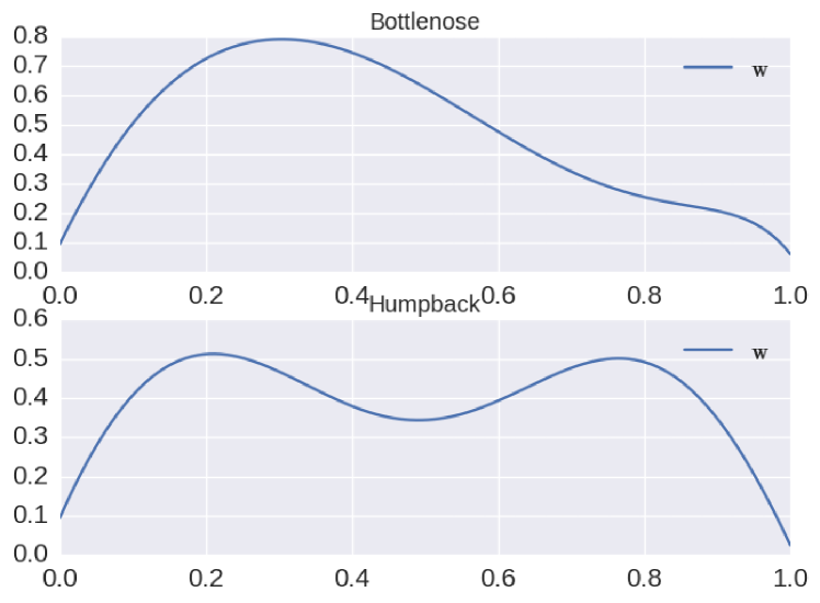
Figure 5: The spatial weight vector $\mathbf{w}$ obtained by performing unconstrained optimization of the top-$k$ score for the Bottlenose dataset (top) and the Humpback dataset (bottom). Note how the weights shrink toward the edges. For the Bottlenose dataset the endpoint of the dorsal fin is often under water. For the Humpback dataset the tips of the fluke are sometimes cropped, and the shortest-path algorithm often skips across the notch.

4.2.2 LNBNN Classification

Similar to [11], we use the local naive Bayes nearest neighbor (LNBNN) algorithm [19] to produce a ranking of known individuals [5]. Our work differs from [11] in that we use the integral curvature representation both to compute descriptors and to determine keypoints.

Feature Descriptor. Instead of using the Difference-of-Gaussian norm defined in Equation 1 in [11] to encode local shape information, we use the curvature representation defined in Section 4.1 of this work. Subsections of the curvature representation are resampled to a fixed length, normalized by the Euclidean norm, and used as feature descriptors.

Feature Keypoints. Similar to [11], we choose the keypoints between which to define the subsections mentioned above by resampling the curvature representation to a fixed length and choosing as keypoints the $n-2$ largest local extrema of the curvature representation at each scale as well as the start and endpoints. Combinations of these keypoints yields ${n}\choose 2$ subsections per scale, between which we extract the corresponding values from the curvature representation.

LNBNN Classification. These feature descriptors are computed for all known individuals in the database, and placed in a data structure for approximate nearest neighbors using ANNOY [3]. We compute a score for each individual using LNBNN classification, specifically Algorithm 2 as defined in [19]. The benefit of using LNBNN instead of standard approximate nearest neighbors is that it considers not only the distance to the nearest descriptor from a given individual, but also the distance to the nearest descriptor from a different individual [5]. The difference between these is used to update the score, which reduces the contribution from non-distinctive feature descriptors.

5 Experiments

To demonstrate the effectiveness of our curvature representation and matching algorithms, we evaluate the two approaches from Section 4.2 for producing a ranking of known individuals on the Bottlenose and Humpback datasets. We use the top-$k$ score, defined as the fraction of the time the correct individual appears in the first $k$ entries of the ranking, to evaluate time-warping (with and without learned spatial weights), as well as LNBNN using our curvature descriptor and the Difference-of-Gaussian descriptor [11].

In particular, we show that when using top-$1$ accuracy, the curvature representation outperforms the Difference-of-Gaussian descriptor by $95\%$ to $91\%$ on the Bottlenose dataset, and $80\%$ to $40\%$ on the Humpback dataset. To compare against Leafsnap [14], we also construct the Histogram of Curvature over Scale from our integral curvature representation, and produce a ranking using the histogram intersection distance. We were unable to achieve good results with this, however, and we suspect that the reason is that computing a histogram over the curvature representation loses the spatial information of the nicks and notches necessary for individual identification.

Additionally, because humpback whales often have uniquely identifying patterns of scarring and pigmentation on their flukes, we also compare against HotSpotter [5], which uses LNBNN with SIFT descriptors [18]. The texture information captured by HotSpotter is complementary to the curvature of the trailing edge, and so we also evaluate combining our identification algorithms with HotSpotter.

We run experiments identical to those described in the following section on two related datasets to ensure the generality of our approach.

5.1 Defining Queries

Bottlenose Dolphins. We randomly select $m=10$ encounters for each individual, and use all the images from these encounters for the database. When an individual appears in only $n$ encounters such that $m>n$, we use $n-1$ encounters for the database so that we have at least one query. The images from remaining encounters are used as query encounters. We also investigate the effect of varying $m$ on the top-$k$ accuracy in Section 5.4.

Humpback Whales. The Humpback dataset typically contains only a single image per individual in each encounter and two encounters per individual. In practice, this means that most individuals are represented by one image in the database.

When evaluating time-warping and HotSpotter, we use the minimum alignment cost across images in the encounter as the similarity score. For LNBNN, we stack the descriptors from all images in the encounter to build the query.

We run all experiments on five random splits and report mean scores, however, there is little variance across runs.

5.2 Qualitative Results

Before quantitatively evaluating our algorithms, we show successful and unsuccessful identifications for the Bottlenose and Humpback datasets in Figures 6 and 7, respectively. In each figure, we show the pair of images (query and database) that contributes the most to the total score. We plot a minimal subset of matches such that the sum of the LNBNN scores from these matches is at least half the total score. Although the matches shown are sparse, in practice the entire length of the contour is matched, albeit with lower scores. Pairs of lines of the same color indicate the start and endpoints of the trailing edge corresponding to the matched curvature descriptor. The matches are ordered such that the strongest match is shown in red, and the weakest in purple. The sections of the trailing edge not covered by strong LNBNN matches is shown in blue.

There are two main causes of misidentifications, namely (a) errors in the contour extraction that cause distinguishing features to be poorly represented in the curvature vectors, and (b) distinctions between very smooth trailing edges that are insufficiently valued by the matching algorithm. Both are amplified by significant viewpoint differences between database and query trailing edges for the correct match.

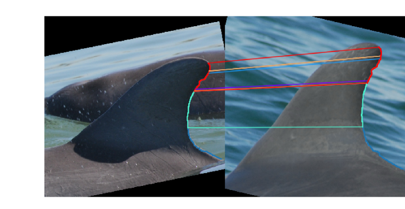
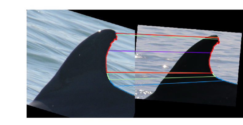
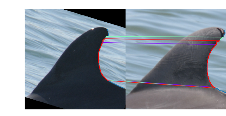
Figure 6: Bottlenose dataset. The top row shows an instance where the correct individual is ranked first. Note how the strongest match (shown in red) corresponds to the most distinct notch. The middle row shows an instance where a different individual is ranked first, while the correct individual, ranked second, is shown in the bottom row. For all rows, we show the query (left) and database (right) images that contribute most to the match score. Weak LNBNN matches are not shown.

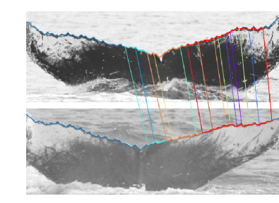
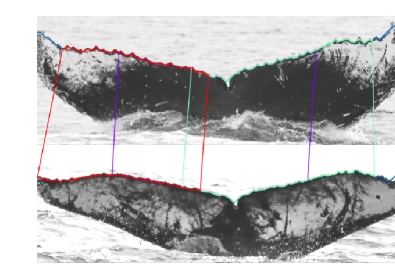
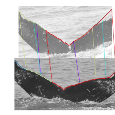
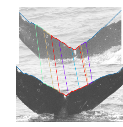
Figure 7: Humpback dataset. The top four images show an instance where the correct individual is ranked first (top left), followed by the database individual ranked second (top right). The bottom four images show an instance where a different individual is ranked first (bottom left), while the correct individual is ranked second (bottom right). For both cases, we show the query (top) and database (bottom) images that contribute most to the total match score. Weak LNBNN matches are not shown.

5.3 Ranking Performance

To evaluate ranking performance, we compare two variations of each of the algorithms from Section 4.2. Next, we describe the parameter choices for each of these algorithms.

Time-Warping Alignment. When using learned spatial weights, we use the relevant $\mathbf{w}$ as shown in Figure 5 for the Bottlenose and Humpback datasets. For the Bottlenose dataset, we resample the curvature representation to $128$ points and set the Sakoe-Chiba bound [23] in the dynamic time-warping algorithm to $8$. We use scales of $\{0.04,0.06,0.08,0.10\}$. For the Humpback dataset, these are set to $748$, $75$, and $\{0.02,0.04,0.06,0.08\}$, respectively. For both datasets, we determine the radii of the circles used for integral curvature (Figure 4) by multiplying the scales by the maximum dimension of the fin, specifically, the height for dorsal fins, and the width for flukes.

Descriptor Indexing. When doing LNBNN classification, we set the number of keypoints at which we define contour subsections to $32$. The keypoints are placed along the trailing edge (which is resampled to $1024$ points) at the points corresponding to the local extrema of the curvature or Difference-of-Gaussian representation, as appropriate. We set the dimension of the feature descriptors to $32$. The top-$k$ accuracy plateaus or slightly degrades on both datasets for larger dimensions. We speculate that this is due to the noisy nature of our extracted trailing edges, where resampling to a smaller feature dimension acts as a form of smoothing. The scales for the Difference-of-Gaussian descriptors are the same as described in [11].

The results for the Bottlenose and Humpback datasets are shown in Figures 8 and 9, respectively. With LNBNN, the curvature descriptor outperforms the Difference-of-Gaussian descriptor for both datasets. We argue that this is because of the robustness with which integral curvature can capture noisy local information --- with a sufficiently large number of points representing the trailing edge, the exact coordinates of any single point have little effect on the curvature value.

Evaluation. The relative performance of the two matching algorithms is different for the two datasets --- it is likely that this is because of how the identifying information is distributed. For the Bottlenose dataset, where only a few distinct marks are useful for identification, the descriptor indexing approach performs better. For the Humpback dataset, where the information necessary for identification is spread along the entire length of the trailing edge, the time-warping alignment approach achieves similar results.

We repeat these experiments on two smaller datasets to determine if our approach generalizes to datasets of the same (or similar) species. On a common dolphin dataset with $3744$ images representing $186$ individuals, we achieve $74\%$ top-$1$ accuracy using time-warping and $69\%$ using LNBNN, and on a humpback whale dataset with $1388$ images representing $419$ individuals, we achieve $86\%$ top-$1$ accuracy using time-warping and $89\%$ using LNBNN.

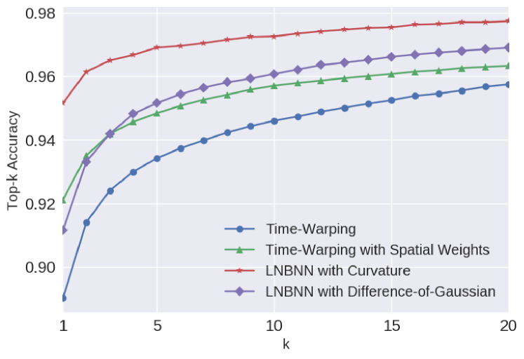
Figure 8: Top-$k$ scores for time-warping alignment and LNBNN for the Bottlenose dataset.

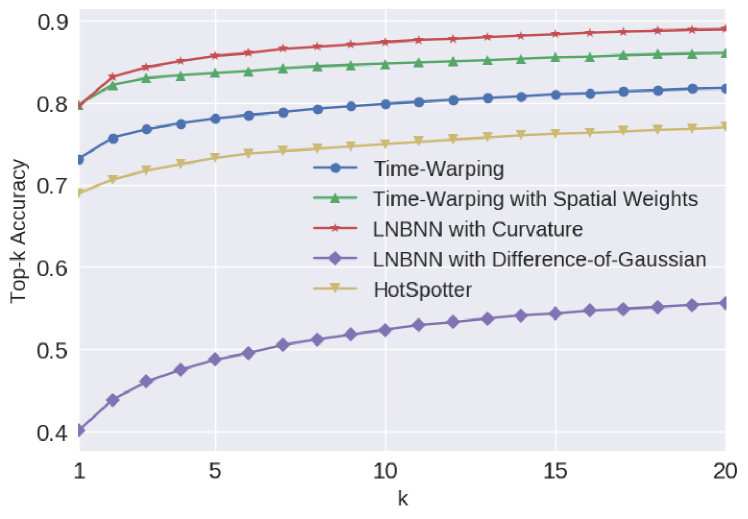
Figure 9: Top-$k$ scores for time-warping alignment, LNBNN, and HotSpotter for the Humpback dataset.

5.4 Number of Encounters per Known Individual

While we choose the encounters from the Bottlenose dataset randomly to evaluate our algorithms, researchers may wish to choose the best images of each known individual for the database. Figure 10 shows the effect of increasing the number of encounters. Adding more encounters, and hence more images, to the database has several advantages. First, there are more viewpoints represented, which makes it more likely that a given query aligns well with one from the database. Second, more images per individual acts as insurance against the event where images may have distinctive parts of the trailing edge occluded. Choosing database images to maximize the information content for identification is a problem we intend to address in future work.

Figure 10: The effect of varying the number of encounters used to represent each individual in the database for the Bottlenose dataset for the two best performing algorithms on this dataset, namely time-warping with spatial weights (TW+SW), as well as LNBNN with curvature descriptors (LNBNN+C).

5.5 Error Correlation

In addition to evaluating the ranking performance of each algorithm separately, we also explore the possibility of combining algorithms. If the correct individual appears in the top-$k$ entries of either of the algorithms, we consider the match to be correct. Combining our algorithms with HotSpotter [5] is of particular interest to us, because of their complementary nature --- while our matching algorithms use the integral curvature of the trailing edge, HotSpotter uses SIFT [18] descriptors extracted from the interior of the fluke to describe the unique patterns of pigmentation. Figure 11 shows that augmenting time-warping (TW+SW) with HotSpotter (HS) improves the top-$1$ accuracy from $80\%$ to $89\%$, and augmenting LNBNN with HotSpotter improves the top-$1$ accuracy from $79\%$ to $88\%$.

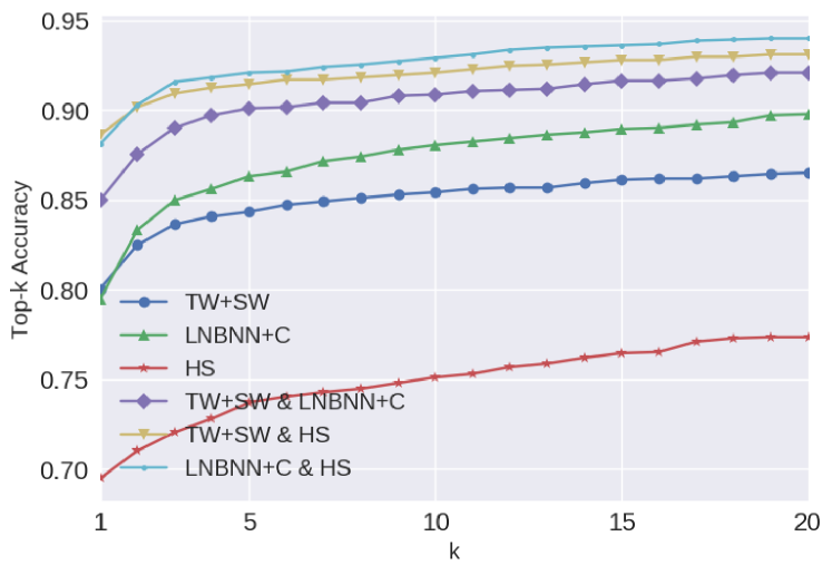
Figure 11: Combining algorithms that use complementary sources of information (fluke pigmentation and trailing edge curvature) improves performance on the Humpback dataset.

6 Conclusion

We introduced novel combinations of integral curvature representation and two matching algorithms for identifying individual cetaceans from their fins. This representation captures the local pattern of nicks and notches in such a way that they may be compared using either a time-warping algorithm or descriptor indexing. The effectiveness of our method is shown by computing accuracy scores on two real-world datasets, each with distinct challenges. For the Bottlenose dataset, with very little information per image, descriptor indexing outperforms time-warping because it considers not only the feature distance, but also distinctiveness. For the Humpback dataset, there are few images per individual, but many features per image. The time-warping algorithm is well-suited for this problem, because it preserves the spatial integrity of curvature along the trailing edge while exploiting learned spatial weights to emphasize matches from regions of stable curvature. As a result, the performance of the two algorithms is similar. In both cases, we demonstrate that we achieve results that can greatly accelerate the process of cetacean identification.

While the focus of this paper has not been on the details of the contour extraction, a major focus of future work will be a unified algorithm that works on both species and leads to a generalization that allows rapid adaptation to new species. An important consideration will be to restrict the amount of manually-generated training data required.

References

- [1] B. Araabi, N. Kehtarnavaz, T. McKinney, G. Hillman, and B. Würsig. A string matching computer-assisted system for dolphin photoidentification. Annals of Biomedical Engineering, 28(10):1269--1279, 2000.
- [2] O. Arandjelovic. Object matching using boundary descriptors. In BMVC, pages 1--11. BMVA Press, 2012.
- [3] E. Bernhardsson. ANNOY: Approximate nearest neighbors in C++/Python optimized for memory usage and loading/saving to disk. https://github.com/spotify/annoy.
- [4] S. Chopra, R. Hadsell, and Y. LeCun. Learning a similarity metric discriminatively, with application to face verification. In CVPR, volume 1, pages 539--546. IEEE, 2005.
- [5] J. P. Crall, C. V. Stewart, T. Y. Berger-Wolf, D. I. Rubenstein, and S. R. Sundaresan. Hotspotter—patterned species instance recognition. In WACV, pages 230--237. IEEE, 2013.
- [6] P. Fischer and T. Brox. Image descriptors based on curvature histograms. In German Conference on Pattern Recognition, pages 239--249. Springer, 2014.
- [7] A. Gilman, T. Dong, K. Hupman, K. Stockin, and M. Pawley. Dolphin fin pose correction using ICP in application to photo-identification. In Image and Vision Computing New Zealand (IVCNZ), 2013 28th International Conference of, pages 388--393. IEEE, 2013.
- [8] P. Hammond. Capturing whales on film--estimating cetacean population parameters from individual recognition data. Mammal Review, 20(1):17--22, 1990.
- [9] G. Hillman, N. Kehtarnavaz, B. Wursig, B. Araabi, G. Gailey, D. Weller, S. Mandava, and H. Tagare. ‘‘Finscan’’, a computer system for photographic identification of marine animals. In EMBS, volume 2, pages 1065--1066. IEEE, 2002.
- [10] E. Hoffer and N. Ailon. Deep metric learning using triplet network. In International Workshop on Similarity-Based Pattern Recognition, pages 84--92. Springer, 2015.
- [11] B. Hughes and T. Burghardt. Automated visual fin identification of individual great white sharks. IJCV, pages 1--16, 2016.
- [12] Z. Jablons. Identifying humpback whale flukes by sequence matching of trailing edge curvature. Master’s thesis, Rensselaer Polytechnic Institute, 2016.
- [13] M. Jaderberg, K. Simonyan, A. Zisserman, et al. Spatial transformer networks. In NIPS, pages 2017--2025, 2015.
- [14] N. Kumar, P. N. Belhumeur, A. Biswas, D. W. Jacobs, W. J. Kress, I. C. Lopez, and J. V. Soares. Leafsnap: A computer vision system for automatic plant species identification. In ECCV, pages 502--516. Springer, 2012.
- [15] B. Leibe and B. Schiele. Analyzing appearance and contour based methods for object categorization. In CVPR, volume 2, pages II--409. IEEE, 2003.
- [16] J. Long, E. Shelhamer, and T. Darrell. Fully convolutional networks for semantic segmentation. In CVPR, pages 3431--3440, 2015.
- [17] G. G. Lorentz. Bernstein polynomials. American Mathematical Soc., 2012.
- [18] D. G. Lowe. Distinctive image features from scale-invariant keypoints. International journal of computer vision, 60(2):91--110, 2004.
- [19] S. McCann and D. G. Lowe. Local naive Bayes nearest neighbor for image classification. In CVPR, pages 3650--3656. IEEE, 2012.
- [20] A. Monroy, A. Eigenstetter, and B. Ommer. Beyond straight lines --- object detection using curvature. In ICIP, pages 3561--3564. IEEE, 2011.
- [21] F. Nogueira. BayesianOptimization. https://github.com/fmfn/BayesianOptimization.
- [22] H. Pottmann, J. Wallner, Q.-X. Huang, and Y.-L. Yang. Integral invariants for robust geometry processing. Computer Aided Geometric Design, 26(1):37--60, 2009.
- [23] H. Sakoe and S. Chiba. Dynamic programming algorithm optimization for spoken word recognition. IEEE transactions on acoustics, speech, and signal processing, 26(1):43--49, 1978.
- [24] R. Stanley. Darwin: identifying dolphins from dorsal fin images. Senior Thesis, Eckerd College, 1995.
- [25] J. Stewman, K. Debure, S. Hale, and A. Russell. Iterative 3-d pose correction and content-based image retrieval for dorsal fin recognition. In International Conference Image Analysis and Recognition, pages 648--660. Springer, 2006.
- [26] Y. Taigman, M. Yang, M. Ranzato, and L. Wolf. Deepface: Closing the gap to human-level performance in face verification. In CVPR, pages 1701--1708, 2014.
- [27] J. Wang, Y. Song, T. Leung, C. Rosenberg, J. Wang, J. Philbin, B. Chen, and Y. Wu. Learning fine-grained image similarity with deep ranking. In CVPR, pages 1386--1393, 2014.
- [28] R. S. Wells and M. D. Scott. Estimating bottlenose dolphin population parameters from individual identification and capture-release techniques. Report of the International Whaling Commission, (12), 1990.
- [29] J. Yosinski, J. Clune, Y. Bengio, and H. Lipson. How transferable are features in deep neural networks? In NIPS, pages 3320--3328, 2014.