Abstract: The transverse momentum distributions of the identified particles produced in small collision systems at the Relativistic Heavy Ion Collider (RHIC) and Large Hadron Collider (LHC) have been analyzed by four models. The first two models utilize the blast-wave model with different statistics. The last two models employ certain linear correspondences based on different distributions. The four models describe the experimental data measured by the Pioneering High Energy Nuclear Interaction eXperiment (PHENIX), Solenoidal Tracker at RHIC (STAR), and A Large Ion Collider Experiment (ALICE) cCollaborations equally well. It is found that both the kinetic freeze-out temperature and transverse flow velocity in the central collisions are comparable with those in the peripheral collisions. With the increase of collision energy from that of the RHIC to that of the LHC, the considered quantities typically do not decrease. Comparing with the central collisions, the proton-proton collisions are closer to the peripheral collisions.

Keywords: kinetic freeze-out temperature, transverse flow velocity, small collision system, central collisions, peripheral collisions

PACS: 25.75.Ag, 25.75.Dw, 24.10.Pa

1 Introduction

As an important concept in both thermal and subatomic physics, temperature is widely used in experimental measurements and theoretical studies. Contrary to macroscopic thermal physics, temperature in microscopic subatomic physics cannot be measured directly; nevertheless, the temperature measured in thermal physics is manifested by the change of a given quantity of the thermometric material. Instead, we can calculate the temperature by using the methods of particle ratios and transverse momentum ($p_{T}$) spectra. The temperature obtained from particle ratios is typically the chemical freeze-out temperature ($T_{ch}$), which can describe the degree of excitation of the interacting system at the stage of chemical equilibrium. The temperature obtained from the $p_{T}$ spectra with a thermal distribution that does not include the flow effect, is typically an effective temperature ($T_{eff}$ or $T$) which is not a real temperature due to its relation to particle mass. The temperature obtained from $p_{T}$ spectra with the thermal distribution which includes flow effect is usually the kinetic freeze-out temperature ($T_{kin}$ or $T_{0}$) which describes the degree of excitation of the interacting system at the stage of kinetic and thermal equilibrium.

The chemical freeze-out and kinetic freeze-out are two main stages of the evolution of the interacting system in high energy collisions. At the stage of chemical freeze-out, the chemical components (relative fractions) of the particles are fixed. At the stage of kinetic freeze-out, the $p_{T}$ and momentum ($p$) spectra of the particles are no longer changed. We are interested in the $T_{0}$ value, owing to its relation to the $p_{T}$ spectrum of the identified particles, which is one of the quantities measured first in our experiments. At the same time, $T_{0}$ is related to the structure of the phase diagram in the $T_{0}$-related spaces, such as $T_{0}$ as a function of $\beta_{T}$ and as a function of $\sqrt{s_{NN}}$, where $\beta_{T}$ is the mean transverse flow velocity, resulted from the impact and squeeze while $\sqrt{s_{NN}}$ denotes the center-of-mass energy per nucleon pair in collisions of nuclei [$\sqrt{s}$ in particle collisions such as in proton-proton ($p$-$p$ or $pp$) collisions]. In particular, in the energy ranges available in the beam energy scan (BES) program at the Relativistic Heavy Ion Collider (RHIC) and the BES program at the Super Proton Synchrotron (SPS), the chemical potential ($\mu_{B}$) of baryons needs to be considered. Then, the structure of phase diagram in the $T_{0}$ versus $\mu_{B}$ space can be studied in both the RHIC BES and the SPS BES energy ranges.

Generally, $\mu_{B}$ can be obtained from the particle ratios and its excitation function has been studied in detail [1–5], while $T_{0}$ and $\beta_{T}$ can be obtained from the $p_{T}$ spectra. In Refs. [6–13], different methods have been used to obtain $T_{0}$ and $\beta_{T}$. In our recent studies [14–17], we have used a number of models to obtain $T_{0}$ and $\beta_{T}$ in nucleus-nucleus [gold-gold (Au-Au) and lead-lead (Pb-Pb)] collisions at the RHIC and Large Hadron Collider (LHC) energies, where the top RHIC energy was $\sqrt{s_{NN}}=200$ GeV while the LHC energy reached a few TeV. Similar results were obtained when a non-zero $\beta_{T}$ was used in peripheral nucleus-nucleus collisions in the Blast-Wave model with Boltzmann-Gibbs statistics (BGBW model) [6–8, 18] and with Tsallis statistics (TBW model) [9, 18, 19]. Our results show that $T_{0}$ ($\beta_{T}$) in central nucleus-nucleus collisions is comparable to that in peripheral collisions. Similarly, the values of $T_{0}$ and $\beta_{T}$ at the LHC are close to those at the RHIC.

It is interesting to compare the results of different models in small collision systems such as $pp$ and deuteron-gold ($d$-Au) collisions at the RHIC, and $pp$ and proton-lead ($p$-Pb) collisions at the LHC. In this paper, we use four models to obtain $T_{0}$ and $\beta_{T}$ values from the $p_{T}$ spectra of the identified particles produced in $pp$ and $d$-Au collisions at the RHIC, and in $pp$ and $p$-Pb collisions at the LHC. The model results of the $p_{T}$ spectra are compared with each other and with the experimental data of the Pioneering High Energy Nuclear Interaction eXperiment (PHENIX) [20], Solenoidal Tracker at RHIC (STAR) [21–23], and A Large Ion Collider Experiment (ALICE) collaborations [24–25]. Then, similar $T_{0}$ and $\beta_{T}$ values are obtained from the analyses of the experimental data by the four models.

The paper is structured as follows. The formalism and method are described in Section 2. Results and discussion are given in Section 3. In Section 4, we summarize our main observations and conclusions.

2 Formalism and method

In the present work, four models were used for the $p_{T}$ distributions for comparisons in small collision systems; nevertheless, in our recent work [14] they were employed to obtain $T_{0}$ and $\beta_{T}$ values in nucleus-nucleus collisions at RHIC and LHC energies using a different superposition of soft excitation and hard scattering components. In order to provide a comprehensive review of the present work, we discuss the previous studies of the four models as follows.

i) BGBW model [6–8]: in this model we considered a non-zero $\beta_{T}$ of the produced particles.

According to refs. [6–8], the BGBW model gives the $p_{T}$ distribution as

$$f_{1}(p_{T}) =\frac{1}{N}\frac{dN}{dp_{T}}=C_{1}p_{T}m_{T}\int_{0}^{R}rdr\times$$

$$I_{0}\bigg{[}\frac{p_{T}\sinh(\rho)}{T_{0}}\bigg{]}K_{1}\bigg{[}\frac{m_{T}\cosh(\rho)}{T_{0}}\bigg{]},$$ (1)

where $N$ is the number of particles, $C_{1}$ is a normalized constant, $I_{0}$ and $K_{1}$ are modified Bessel functions of the first and second kinds, respectively, $m_{T}=\sqrt{p_{T}^{2}+m_{0}^{2}}$ is the transverse mass, $\rho=\tanh^{-1}[\beta(r)]$ is the boost angle, $\beta(r)=\beta_{S}(r/R)^{n_{0}}$ is a self-similar flow profile, $\beta_{S}$ is the flow velocity on the surface, $r/R$ is the relative radial position in the thermal source [6], and $n_{0}=2$ similarly to that in ref. [6]. The relation between $\beta_{T}$ and $\beta(r)$ is $\beta_{T}=(2/R^{2})\int_{0}^{R}r\beta(r)dr=2\beta_{S}/(n_{0}+2)=0.5\beta_{S}$.

ii) TBW model [9]: in this model we also considered a non-zero $\beta_{T}$.

According to refs. [9], the TBW model gives the $p_{T}$ distribution in the form of

$$f_{2}(p_{T}) =\frac{1}{N}\frac{dN}{dp_{T}}=C_{2}p_{T}m_{T}\int_{-\pi}^{\pi}d\phi\int_{0}^{R}rdr\Big{\{}1+$$

$$\frac{q-1}{T_{0}}\big{[}m_{T}\cosh(\rho)-p_{T}\sinh(\rho)\cos(\phi)\big{]}\Big{\}}^{-q/(q-1)},$$ (2)

where $C_{2}$ is a normalized constant, $q$ is an entropy index characterizing the degree of non-equilibrium, $\phi$ denotes the azimuth [9], and $n_{0}=1$ similarly to that in ref. [9]. In the first two models, $n_{0}$ is independent: it does not matter if $n_{0}=1$ or $n_{0}=2$ is used. To be compatible with refs. [6] and [9], we use $n_{0}=2$ in the first model and $n_{0}=1$ in the second model. It should be noted that we use the index $-q/(q-1)$ in Eq. (2) instead of $-1/(q-1)$ in ref. [9] due to the fact that $q$ is very close to one. This substitution results in a small and negligible difference in the Tsallis distribution [19].

iii) An alternative method, in which the intercept in the $T$ versus $m_{0}$ relation is assumed to be $T_{0}$ [7, 10–13], the slope in the $\langle p_{T}\rangle$ versus $\overline{m}$ relation is assumed to be $\beta_{T}$, and the slope in the $\langle p\rangle$ versus $\overline{m}$ relation is assumed to be the radial flow velocity $\beta$ [14–17], which does not include the contribution of longitudinal flow. Here $m_{0}$ denotes the rest mass, $\overline{m}$ denotes the mean moving mass (mean energy), $\langle...\rangle$ denotes the theoretical distribution average of the considered quantity, and $T$ is obtained from a Boltzmann distribution [18].

Two steps are required to obtain $T_{0}$ and $\beta_{T}$. To use the relations $T=T_{0}+am_{0}$, $\langle p_{T}\rangle=b_{1}+\beta_{T}\overline{m}$, and $\langle p\rangle=b_{2}+\beta\overline{m}$, where $a$, $b_{1}$, and $b_{2}$ are fitted parameters, we choose the form of Boltzmann distribution as [18]

$$f_{3}(p_{T})=\frac{1}{N}\frac{dN}{dp_{T}}=C_{3}p_{T}m_{T}\exp\bigg{(}-\frac{m_{T}}{T}\bigg{)},$$ (3)

where $C_{3}$ is a normalized constant related to the free parameter $T$ and particle mass $m_{0}$ via its relation to $m_{T}$; nevertheless, the Boltzmann distribution has multiple forms [18].

iv) This model is similar to the third model, but $T$ is obtained from a Tsallis distribution [18, 19].

We choose the Tsallis distribution in the form of [18, 19]

$$f_{4}(p_{T})=\frac{1}{N}\frac{dN}{dp_{T}}=C_{4}p_{T}m_{T}\bigg{(}1+\frac{q-1}{T}m_{T}\bigg{)}^{-q/(q-1)},$$ (4)

where $C_{4}$ is a normalized constant related to the free parameters $T$ and $q$, as well as $m_{0}$; nevertheless, the Tsallis distribution has more than one forms [18, 19].

Similarly to our recent work [14], in both the BGBW and TBW models, a non-zero $\beta_{T}$ of the produced particles is considered in the peripheral nucleus-nucleus collisions. The peripheral collisions contain a small number of participant nucleons that take part in the violent interactions. This condition is similar to a small collision system, which also contains a small number of participant nucleons. When the cold nuclear effect is neglected, the small collision system is similar to a peripheral collisions. This means that a non-zero $\beta_{T}$ needs to be considered for the small collision system to maintain consistency; however, the values of $\beta_{T}$ for a small collision system and peripheral collisions are possibly different. Naturally, it is not unusual if the values of $\beta_{T}$ in the two types of collisions are nearly the same.

From the first model $T_{0}$ and $\beta_{T}$ can be obtained, while from the second model $T_{0}$, $\beta_{T}$, and $q$ can be obtained. The first two models are employed to compare their results. Although the forms of the first two models are obviously different, the values of $T_{0}$ ($\beta_{T}$) obtained from them exhibit a little difference only. The last two models are used for comparison as well. The obtained values of the last two models exhibit a little difference as well; however they are still noticeably different.

The description of the above models is presented at mid-rapidity, in which $y\approx 0$, where $y\equiv 0.5\ln[(E+p_{z})/(E-p_{z})]$, and $E$ and $p_{z}$ denote the energy and longitudinal momentum, respectively. At high $p_{T}$, $y\approx-\ln\tan(\vartheta/2)\equiv\eta$, where $\vartheta$ and $\eta$ denote the emission angle and pseudorapidity of the considered particle, respectively. The effect of the spin and chemical potential on the $p_{T}$ spectra is neglected because they are small at the top RHIC and LHC energies [1–4]. Similarly to our recent work [14], the kinetic freeze-out temperature, the mean transverse (radial) flow velocity, and the effective temperature in different models are uniformly denoted by $T_{0}$, $\beta_{T}$, and $T$, respectively; however, different values can be obtained by different models.

Equations (1)–(4) are the functions describing mainly the contribution of the soft excitation process. These are only valid for the spectra in a narrow $p_{T}$ range, which mainly covers the range mainly from 0 to 2.5–3.5 GeV/$c$ in most cases or a slightly higher in certain cases. Even for the soft excitation process, the Boltzmann distribution is not sufficient to fit the $p_{T}$ spectra in certain cases. In the case of a two- or three-component Boltzmann distribution, $T$ is the weighted average resulting from different effective temperatures and the corresponding fractions obtained from different components.

Generally, in the present work, two main processes in high energy collisions are considered. Apart from the soft excitation process, the main process is the hard scattering process, which contributes to the spectra in a wide $p_{T}$ range and according to the quantum chromodynamics (QCD) calculation [26–28], it can be described by an inverse power-law as

$$f_{H}(p_{T})=\frac{1}{N}\frac{dN}{dp_{T}}=Ap_{T}\bigg{(}1+\frac{p_{T}}{p_{0}}\bigg{)}^{-n},$$ (5)

where $p_{0}$ and $n$ are free parameters, and $A$ is a normalized constant related to the free parameters. As a result of the QCD-based calculation, Eq. (5) contributes to the distribution in a range of 0 to high $p_{T}$. Theoretically, in spite of the overlapping regions in the low $p_{T}$ range between the contributions of Eqs. (1)–(4) and (5), they cannot replace each other.

The experimental $p_{T}$ spectra are typically distributed in a wide range. This means that a superposition of both the contributions of soft and hard processes (components) needs to be used to fit the spectra. We use the usual step function for structuring the superposition in order to avoid the entanglement between the contribution ranges of the soft excitation and hard scattering components, such that

$$f_{0}(p_{T}) =\frac{1}{N}\frac{dN}{dp_{T}}=A_{1}\theta(p_{1}-p_{T})f_{S}(p_{T})$$

$$+A_{2}\theta(p_{T}-p_{1})f_{H}(p_{T}),$$ (6)

where $f_{S}(p_{T})$ denotes one of Eqs. (1)–(4), $A_{1}$ and $A_{2}$ are constants, ensuring that the contributions of soft and hard components are the same at $p_{T}=p_{1}$, and the step function $\theta(x)=1$ if $x>0$ and $\theta(x)=0$ if $x<0$. The fraction (rate) of the contribution of the soft component is given by $k=\int_{0}^{p_{1}}A_{1}f_{S}(p_{T})dp_{T}$. Owing to the respective ranges of the different contributions, the selection of parameters in Eqs. (1)–(4) and (5) has no effect on their correlation and dependence on each other.

In certain cases, the contribution of the resonance production for pions and the strong stopping effect for the participating nucleons are non-negligible at very low ranges. A very-soft component needs to be used for the $p_{T}$ values ranging from 0 to 0.5–1.5 GeV/$c$. Let us consider the contribution of the very-soft component. Equation (6) can be rewritten as

$$f_{0}(p_{T}) =\frac{1}{N}\frac{dN}{dp_{T}}=A_{VS}\theta(p_{VS}-p_{T})f_{VS}(p_{T})$$

$$+A_{1}\theta(p_{T}-p_{VS})\theta(p_{1}-p_{T})f_{S}(p_{T})$$

$$+A_{2}\theta(p_{T}-p_{1})f_{H}(p_{T}),$$ (7)

where $f_{VS}(p_{T})$ denotes one of Eqs. (1)–(4) similarly to $f_{S}(p_{T})$, and $A_{VS}$ is a constant ensuring that the contributions of the very-soft and soft components are the same at $p_{T}=p_{VS}$. Let us denote the rates of the very-soft and soft components by $k_{VS}$ and $k_{S}$, respectively. Then, $k_{VS}=\int_{0}^{p_{VS}}A_{VS}f_{VS}(p_{T})dp_{T}$ and $k_{S}=\int_{p_{VS}}^{p_{1}}A_{1}f_{S}(p_{T})dp_{T}$, where $k_{VS}+k_{S}=k$ [for the definition of $k$, please refer to the section following Eq. (6)].

Although $f_{VS}(p_{T})$ and $f_{S}(p_{T})$ have the same form in Eq. (7), their contribution ranges are different. Similarly, the contribution range of $f_{H}(p_{T})$ is different from those of $f_{VS}(p_{T})$ and $f_{S}(p_{T})$. The three functions have no correlation or dependence in the fitting procedure. We fitted $f_{VS}(p_{T})$ at very-soft $p_{T}$ ranging from 0 to 0.5–1.5 GeV/$c$, $f_{S}(p_{T})$ at soft $p_{T}$ ranging from 0.5–1.5 GeV/$c$ to 2.5–3.5 GeV/$c$, and $f_{H}(p_{T})$ at hard $p_{T}$ ranging from 2.5–3.5 GeV/$c$ to the maximum. In the case of without $f_{VS}(p_{T})$, Eq. (7) transforms into Eq. (6). Then, we fitted $f_{S}(p_{T})$ in Eq. (6) in the range of 0 to 2.5–3.5 GeV/$c$. In the calculation, because of their different fractions, we used the weighted average of parameters in very-soft and soft components in Eq. (7) to compare them with the values obtained from Eqs. (6) and (7).

3 Results and discussion

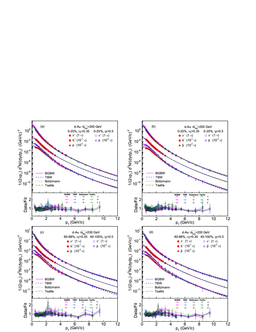
Figure 1: (Color online) Transverse momentum spectra of $\pi^{+}$, $K^{+}$, and $p$ [panels (a) and (c)], as well as $\pi^{-}$, $K^{-}$, and $\bar{p}$ [panels (b) and (d)] produced in 0–20% [panels (a) and (b)] and 60–88% (40–100%) [panels (c) and (d)] $d$-Au collisions at $\sqrt{s_{NN}}=200$ GeV. For clarity, the spectra for different particles are multiplied by different amounts shown in the panels. The closed and open symbols represent the experimental data of the PHENIX and STAR collaborations measured in $|\eta|<0.35$ [20] and $|y|<0.5$ [21], respectively. The solid, dashed, dotted, and dashed-dotted curves are our results fitted by Eqs. (6) and (7) in which $f_{S}(p_{T})$ ($f_{VS}(p_{T})$) denote $f_{1}(p_{T})$, $f_{2}(p_{T})$, $f_{3}(p_{T})$, and $f_{4}(p_{T})$, respectively. The bottom panels show the data for the fitting of the ratios.

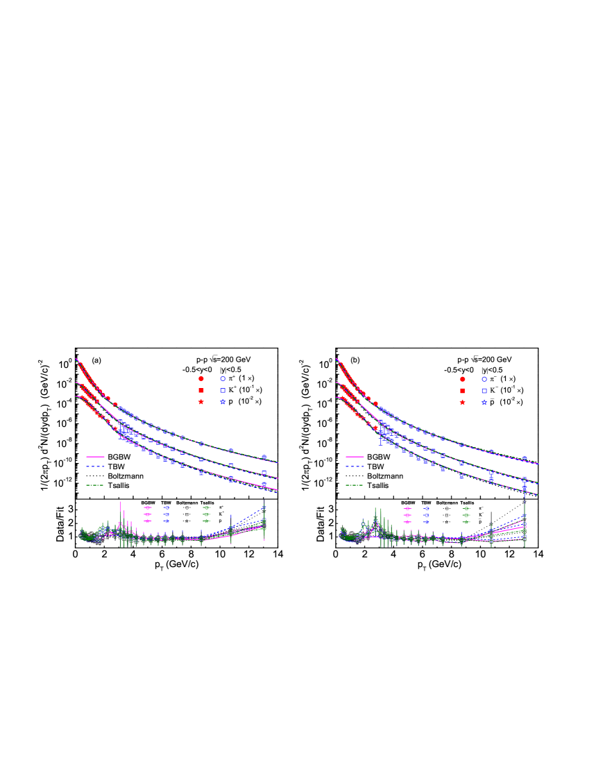
Figure 2: (Color online) Spectra of $\pi^{+}$, $K^{+}$, and $p$ (panel (a)), as well as $\pi^{-}$, $K^{-}$, and $\bar{p}$ (panels (b)), produced in $pp$ collisions at $\sqrt{s}=200$ GeV. The closed and open symbols represent the experimental data of the STAR collaboration measured in $-0.5<y<0$ and $|y|<0.5$, respectively [22, 23].

In Fig. 1, the transverse momentum spectra, $1/(2\pi p_{T})\cdot d^{2}N/(dydp_{T})$, are shown for positively charged pions ($\pi^{+}$), positively charged kaons ($K^{+}$), and protons ($p$) [Figs. 1(a) and 1(c)], as well as negatively charged pions ($\pi^{-}$), negatively charged kaons ($K^{-}$), and antiprotons ($\bar{p}$) [Figs. 1(b) and 1(d)] produced in 0–20% [Figs. 1(a) and 1(b)] and 60–88% (40–100%) [Figs. 1(c) and 1(d)] $d$-Au collisions at $\sqrt{s_{NN}}=200$ GeV. The closed and open symbols represent the experimental data of the PHENIX and STAR Collaboration measured in the pseudorapidity range $|\eta|<0.35$ [20] and the rapidity range $|y|<0.5$ [21], respectively. The curves show the results obtained by models i)–iv) and the fit parameters are given in Tables 1–4, respectively, with most of them are fitted by Eq. (6). The numerical values fitted by Eq. (7) are marked by a star at the end of the line, where the results obtained from the very-soft and soft components are shown together. It can be seen that the four considered models describe the $p_{T}$ spectra of the identified particles produced in central (0–20%) and peripheral (60–88% and 40–100%) $d$-Au collisions at $\sqrt{s_{NN}}=200$ GeV similarly well.

Similarly to Fig. 1, Figs. 2(a) and 2(b) show the spectra of $\pi^{+}$, $K^{+}$, and $p$, as well as $\pi^{-}$, $K^{-}$, and $\bar{p}$, produced in $pp$ collisions at $\sqrt{s}=200$ GeV. The closed and open symbols represent the experimental data of the STAR collaboration measured in the range of $-0.5<y<0$ and at $|y|<0.5$, respectively [22, 23]. The fitting parameters are given in Tables 1–4. It can be seen that the four considered models describe the $p_{T}$ spectra of the identified particles produced in $pp$ collisions at $\sqrt{s}=200$ GeV similarly well.

Figure 3 is similar to Fig. 1, and it shows the spectra of $\pi^{+}+\pi^{-}$, $K^{+}+K^{-}$, and $p+\bar{p}$ produced in 0–5% [Fig. 3(a)] and 80–100% [Fig. 3(b)] $p$-Pb collisions at $\sqrt{s_{NN}}=5.02$ TeV. The symbols represent the experimental data of the ALICE collaboration measured in the range of $-0.5<y<0$ [24]. It can be seen in most cases that the four considered models describe the $p_{T}$ spectra of the identified particles produced in $p$-Pb collisions at $\sqrt{s_{NN}}=5.02$ TeV similarly well.

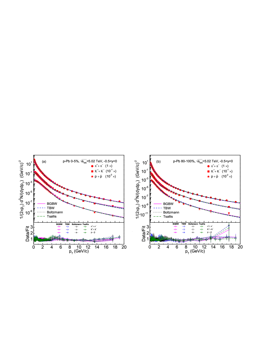
Figure 3: (Color online) Spectra of $\pi^{+}+\pi^{-}$, $K^{+}+K^{-}$, and $p+\bar{p}$ produced in 0–5% [panel (a)] and 80–100% [panel (b)] $p$-Pb collisions at $\sqrt{s_{NN}}=5.02$ TeV. The symbols represent the experimental data of the ALICE collaboration measured in the range of $-0.5<y<0$ [24].

Similarly to Fig. 1, Fig. 4 shows spectra, $(1/N_{EV})\cdot 1/(2\pi p_{T})\cdot d^{2}N/(dydp_{T})$, of $\pi^{+}+\pi^{-}$, $K^{+}+K^{-}$, and $p+\bar{p}$ produced in $pp$ collisions at $\sqrt{s}=2.76$ TeV, where $N_{EV}$ denotes the number of events and it is typically omitted. The symbols represent the experimental data of the ALICE collaboration measured in $|y|<0.5$ for low-$p_{T}$ particles and in $|\eta|<0.8$ for high-$p_{T}$ particles [25]. The four considered models describe the $p_{T}$ spectra of the identified particles produced in $pp$ collisions at $\sqrt{s}=2.76$ TeV similarly well in most of the cases.

Table 1. Values of parameters ($T_{0}$, $\beta_{T}$, $k$, $p_{0}$, and $n$), normalization constant ($N_{0}$), $\chi^{2}$, and degrees of freedom (DOF) corresponding to the fits of the BGBW model and the inverse power-law [Eqs. (1) and (5) through Eq. (6) or (7)] in Figs. 1–4 and 8. For better readability, the collision types, data sources, and collision energies are listed in the blank spaces of the first two columns. The results of the very-soft and soft components are listed together and marked by an asterisk (*) at the end of the line.

Figure	Centrality	Particle	$T_{0}$ (GeV)	$\beta_{T}$ ($c$)	$k$	$p_{0}$ (GeV/$c$)	$n$	$N_{0}$	$\chi^{2}$/DOF
1(a)	0–20%	$\pi^{+}$	$0.112\pm 0.006$	$0.43\pm 0.01$	$0.999\pm 0.001$	$5.0\pm 0.3$	$15.9\pm 0.4$	$4.85\pm 0.51$	37/18
$d$-Au	200 GeV	$K^{+}$	$0.128\pm 0.008$	$0.42\pm 0.01$	$0.994\pm 0.006$	$5.8\pm 0.3$	$16.5\pm 0.4$	$0.64\pm 0.07$	9/15
PHENIX		$p$	$0.130\pm 0.008$	$0.39\pm 0.01$	$0.998\pm 0.002$	$5.2\pm 0.3$	$15.2\pm 0.4$	$0.30\pm 0.02$	64/18
1(b)	0–20%	$\pi^{-}$	$0.121\pm 0.006$	$0.43\pm 0.01$	$0.999\pm 0.001$	$5.4\pm 0.3$	$16.7\pm 0.4$	$4.30\pm 0.50$	23/18
		$K^{-}$	$0.121\pm 0.008$	$0.43\pm 0.01$	$0.995\pm 0.004$	$6.1\pm 0.3$	$17.3\pm 0.4$	$0.60\pm 0.06$	7/15
		$\bar{p}$	$0.129\pm 0.008$	$0.39\pm 0.01$	$0.999\pm 0.001$	$5.1\pm 0.2$	$16.1\pm 0.4$	$0.24\pm 0.02$	103/18
1(c)	60–88%	$\pi^{+}$	$0.104\pm 0.006$	$0.43\pm 0.01$	$0.998\pm 0.002$	$3.5\pm 0.2$	$12.9\pm 0.3$	$1.29\pm 0.14$	30/18
		$K^{+}$	$0.116\pm 0.008$	$0.41\pm 0.01$	$0.982\pm 0.008$	$6.4\pm 0.2$	$17.2\pm 0.4$	$0.15\pm 0.02$	12/15
		$p$	$0.119\pm 0.009$	$0.37\pm 0.01$	$0.996\pm 0.004$	$5.5\pm 0.2$	$15.6\pm 0.3$	$0.07\pm 0.01$	33/18
1(d)	60–88%	$\pi^{-}$	$0.104\pm 0.006$	$0.43\pm 0.01$	$0.998\pm 0.002$	$3.5\pm 0.2$	$12.9\pm 0.3$	$1.29\pm 0.08$	36/18
		$K^{-}$	$0.115\pm 0.008$	$0.40\pm 0.01$	$0.983\pm 0.011$	$6.0\pm 0.2$	$17.2\pm 0.3$	$0.15\pm 0.02$	15/15
		$\bar{p}$	$0.119\pm 0.008$	$0.37\pm 0.01$	$0.997\pm 0.003$	$5.5\pm 0.2$	$16.6\pm 0.3$	$0.05\pm 0.01$	31/18
1(a)	0–20%	$\pi^{+}$	$0.111\pm 0.006$	$0.43\pm 0.01$	$0.999\pm 0.001$	$4.4\pm 0.2$	$15.3\pm 0.3$	$9.20\pm 0.99$	21/18
$d$-Au	200 GeV	$p$	$0.128\pm 0.008$	$0.37\pm 0.01$	$0.998\pm 0.002$	$5.1\pm 0.2$	$15.9\pm 0.3$	$0.97\pm 0.10$	18/16
1(b)	0–20%	$\pi^{-}$	$0.111\pm 0.006$	$0.43\pm 0.01$	$0.999\pm 0.001$	$4.4\pm 0.2$	$15.3\pm 0.3$	$9.2\pm 1.00$	24/18
STAR		$\bar{p}$	$0.127\pm 0.005$	$0.37\pm 0.01$	$0.998\pm 0.002$	$5.1\pm 0.1$	$16.9\pm 0.2$	$0.79\pm 0.09$	21/16
1(c)	40–100%	$\pi^{+}$	$0.103\pm 0.006$	$0.42\pm 0.01$	$0.999\pm 0.001$	$3.7\pm 0.2$	$13.4\pm 0.3$	$2.78\pm 0.28$	26/18
		$p$	$0.115\pm 0.007$	$0.37\pm 0.01$	$0.998\pm 0.002$	$6.9\pm 0.1$	$18.2\pm 0.3$	$0.25\pm 0.03$	33/16
1(d)	40–100%	$\pi^{-}$	$0.103\pm 0.006$	$0.42\pm 0.01$	$0.999\pm 0.001$	$3.7\pm 0.2$	$13.4\pm 0.3$	$2.78\pm 0.28$	22/18
		$\bar{p}$	$0.112\pm 0.006$	$0.35\pm 0.01$	$0.998\pm 0.002$	$6.4\pm 0.1$	$18.9\pm 0.3$	$0.24\pm 0.02$	39/16
2(a)		$\pi^{+}$	$0.104\pm 0.006$	$0.40\pm 0.01$	$0.999\pm 0.001$	$2.2\pm 0.1$	$11.2\pm 0.3$	$0.64\pm 0.07$	22/23
$pp$	200 GeV	$K^{+}$	$0.114\pm 0.008$	$0.41\pm 0.01$	$0.999\pm 0.001$	$3.0\pm 0.1$	$12.4\pm 0.3$	$0.07\pm 0.01$	8/18
STAR		$p$	$0.116\pm 0.008$	$0.34\pm 0.01$	$0.999\pm 0.001$	$3.1\pm 0.2$	$12.6\pm 0.3$	$0.05\pm 0.01$	29/22
2(b)		$\pi^{-}$	$0.104\pm 0.006$	$0.40\pm 0.01$	$0.999\pm 0.001$	$2.2\pm 0.1$	$11.3\pm 0.3$	$0.64\pm 0.07$	27/23
		$K^{-}$	$0.114\pm 0.008$	$0.41\pm 0.01$	$0.999\pm 0.001$	$3.2\pm 0.1$	$13.5\pm 0.3$	$0.07\pm 0.01$	4/18
		$\bar{p}$	$0.116\pm 0.008$	$0.34\pm 0.01$	$0.998\pm 0.002$	$3.1\pm 0.2$	$13.7\pm 0.4$	$0.04\pm 0.01$	46/22
3(a)	0–5%	$\pi^{\pm}$	$0.136\pm 0.008$	$0.43\pm 0.01$	$0.999\pm 0.001$	$2.1\pm 0.1$	$7.6\pm 0.3$	$18.70\pm 1.99$	320/49*
$p$-Pb	5.02 TeV	$K^{\pm}$	$0.193\pm 0.009$	$0.43\pm 0.01$	$0.997\pm 0.003$	$2.7\pm 0.1$	$7.3\pm 0.3$	$2.84\pm 0.41$	71/45
ALICE		$p$+$\bar{p}$	$0.195\pm 0.009$	$0.42\pm 0.01$	$0.999\pm 0.001$	$3.5\pm 0.2$	$8.8\pm 0.3$	$1.10\pm 0.11$	172/43
3(b)	80–100%	$\pi^{\pm}$	$0.112\pm 0.008$	$0.43\pm 0.01$	$0.988\pm 0.006$	$1.3\pm 0.1$	$7.4\pm 0.3$	$1.91\pm 0.20$	234/52
		$K^{\pm}$	$0.139\pm 0.008$	$0.41\pm 0.01$	$0.990\pm 0.006$	$3.3\pm 0.1$	$8.9\pm 0.3$	$0.25\pm 0.02$	119/45
		$p$+$\bar{p}$	$0.156\pm 0.009$	$0.37\pm 0.01$	$0.993\pm 0.006$	$3.9\pm 0.1$	$10.1\pm 0.3$	$0.10\pm 0.01$	225/43
4		$\pi^{\pm}$	$0.111\pm 0.008$	$0.43\pm 0.01$	$0.994\pm 0.005$	$1.9\pm 0.1$	$8.1\pm 0.3$	$3.60\pm 0.35$	382/57
$pp$	2.76 TeV	$K^{\pm}$	$0.143\pm 0.008$	$0.42\pm 0.01$	$0.990\pm 0.005$	$2.9\pm 0.1$	$8.6\pm 0.3$	$0.45\pm 0.05$	119/52
ALICE		$p$+$\bar{p}$	$0.152\pm 0.009$	$0.36\pm 0.01$	$0.991\pm 0.005$	$2.6\pm 0.1$	$9.5\pm 0.3$	$0.19\pm 0.01$	214/43
8(a)	0–20%	$\pi^{\pm}$	$0.107\pm 0.006$	$0.41\pm 0.01$	$0.999\pm 0.001$	$4.4\pm 0.3$	$14.5\pm 0.4$	$103.61\pm 11.37$	28/23
Cu-Cu	200 GeV	$K^{\pm}$	$0.122\pm 0.011$	$0.41\pm 0.02$	$0.997\pm 0.003$	$6.1\pm 0.3$	$16.3\pm 0.4$	$12.52\pm 1.26$	1/10
		$p$+$\bar{p}$	$0.125\pm 0.008$	$0.38\pm 0.01$	$0.999\pm 0.001$	$5.2\pm 0.3$	$15.7\pm 0.4$	$7.85\pm 0.77$	5/21
8(b)	40–94%	$\pi^{\pm}$	$0.101\pm 0.005$	$0.43\pm 0.01$	$0.999\pm 0.001$	$4.3\pm 0.2$	$14.5\pm 0.3$	$8.29\pm 0.81$	18/23
		$K^{\pm}$	$0.111\pm 0.008$	$0.40\pm 0.01$	$0.996\pm 0.003$	$5.9\pm 0.2$	$16.9\pm 0.3$	$1.28\pm 0.11$	1/10
		$p$+$\bar{p}$	$0.114\pm 0.009$	$0.37\pm 0.01$	$0.996\pm 0.003$	$6.4\pm 0.2$	$19.9\pm 0.2$	$0.50\pm 0.05$	15/21

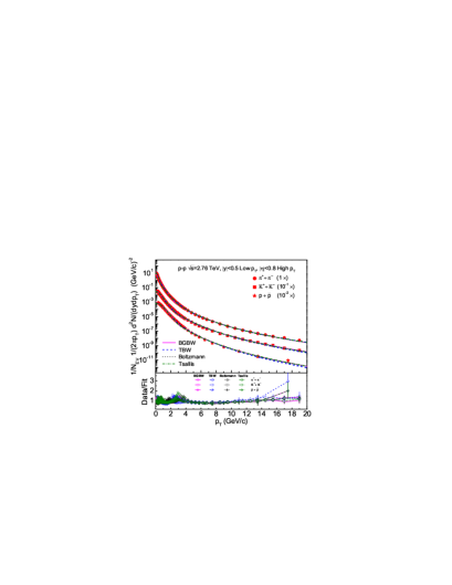
Figure 4: (Color online) Spectra of $\pi^{+}+\pi^{-}$, $K^{+}+K^{-}$, and $p+\bar{p}$ produced in $pp$ collisions at $\sqrt{s}=2.76$ TeV. The symbols represent the experimental data of the ALICE collaboration measured in $|y|<0.5$ for low-$p_{T}$ particles and in $|\eta|<0.8$ for high-$p_{T}$ particles [25].

Table 2. Values of parameters ($T_{0}$, $q$, $\beta_{T}$, $k$, $\ p_{0}$, and $n$), normalization constant ($N_{0}$), $\chi^{2}$, and DOF corresponding to the fits of the TBW model and the inverse power-law [Eqs. (2) and (5) through Eq. (6) or (7)] in Figs. 1–4 and 8, where the columns of centrality and particle are the same as those in Table 1; thus, these are omitted.

Figure	$T_{0}$ (GeV)	$q$	$\beta_{T}$ ($c$)	$k$	$p_{0}$ (GeV/$c$)	$n$	$N_{0}$	$\chi^{2}$/DOF
1(a)	$0.108\pm 0.006$	$1.025\pm 0.007$	$0.46\pm 0.01$	$0.991\pm 0.005$	$4.8\pm 0.3$	$16.2\pm 0.4$	$3.86\pm 0.39$	46/17
$d$-Au	$0.118\pm 0.008$	$1.026\pm 0.008$	$0.46\pm 0.01$	$0.981\pm 0.006$	$5.9\pm 0.3$	$16.0\pm 0.4$	$0.57\pm 0.06$	24/14
PHENIX	$0.119\pm 0.008$	$1.018\pm 0.007$	$0.45\pm 0.01$	$0.996\pm 0.004$	$5.1\pm 0.2$	$15.9\pm 0.4$	$0.25\pm 0.02$	19/17
1(b)	$0.108\pm 0.006$	$1.025\pm 0.007$	$0.46\pm 0.01$	$0.992\pm 0.005$	$4.8\pm 0.3$	$16.4\pm 0.4$	$3.86\pm 0.39$	56/17
	$0.118\pm 0.008$	$1.026\pm 0.008$	$0.46\pm 0.01$	$0.983\pm 0.009$	$5.9\pm 0.3$	$17.0\pm 0.4$	$0.57\pm 0.06$	34/14
	$0.118\pm 0.008$	$1.018\pm 0.007$	$0.45\pm 0.01$	$0.996\pm 0.004$	$5.1\pm 0.2$	$16.3\pm 0.4$	$0.20\pm 0.02$	36/17
1(c)	$0.088\pm 0.006$	$1.045\pm 0.008$	$0.46\pm 0.01$	$0.994\pm 0.004$	$3.5\pm 0.2$	$13.7\pm 0.3$	$1.02\pm 0.10$	34/17
	$0.090\pm 0.008$	$1.029\pm 0.008$	$0.46\pm 0.01$	$0.955\pm 0.011$	$6.4\pm 0.3$	$17.5\pm 0.4$	$0.13\pm 0.01$	9/14
	$0.098\pm 0.008$	$1.012\pm 0.007$	$0.44\pm 0.01$	$0.990\pm 0.006$	$5.5\pm 0.2$	$15.9\pm 0.2$	$0.06\pm 0.01$	37/17
1(d)	$0.088\pm 0.006$	$1.045\pm 0.008$	$0.46\pm 0.01$	$0.994\pm 0.006$	$3.5\pm 0.2$	$13.7\pm 0.3$	$1.02\pm 0.10$	46/17
	$0.090\pm 0.008$	$1.029\pm 0.008$	$0.46\pm 0.01$	$0.957\pm 0.011$	$6.7\pm 0.3$	$18.6\pm 0.4$	$0.13\pm 0.01$	11/14
	$0.097\pm 0.008$	$1.012\pm 0.007$	$0.43\pm 0.01$	$0.992\pm 0.006$	$5.5\pm 0.2$	$17.1\pm 0.3$	$0.05\pm 0.01$	48/17
1(a)	$0.106\pm 0.006$	$1.020\pm 0.008$	$0.46\pm 0.01$	$0.995\pm 0.004$	$4.4\pm 0.2$	$15.6\pm 0.4$	$7.07\pm 0.76$	38/17
$d$-Au	$0.115\pm 0.008$	$1.010\pm 0.007$	$0.38\pm 0.01$	$0.998\pm 0.002$	$4.4\pm 0.2$	$15.6\pm 0.4$	$0.96\pm 0.10$	35/11*
1(b)	$0.106\pm 0.006$	$1.020\pm 0.008$	$0.46\pm 0.01$	$0.995\pm 0.004$	$4.4\pm 0.2$	$15.6\pm 0.4$	$7.07\pm 0.76$	39/17
STAR	$0.116\pm 0.008$	$1.008\pm 0.005$	$0.44\pm 0.01$	$0.997\pm 0.003$	$5.1\pm 0.2$	$17.7\pm 0.4$	$0.73\pm 0.07$	44/15
1(c)	$0.085\pm 0.006$	$1.038\pm 0.008$	$0.46\pm 0.01$	$0.996\pm 0.004$	$3.7\pm 0.2$	$13.9\pm 0.3$	$2.50\pm 0.25$	33/17
	$0.090\pm 0.008$	$1.008\pm 0.007$	$0.35\pm 0.01$	$0.998\pm 0.002$	$6.9\pm 0.2$	$19.6\pm 0.4$	$0.31\pm 0.02$	29/11*
1(d)	$0.085\pm 0.006$	$1.038\pm 0.008$	$0.46\pm 0.01$	$0.996\pm 0.004$	$3.7\pm 0.2$	$13.9\pm 0.3$	$2.54\pm 0.25$	48/17
	$0.094\pm 0.008$	$1.016\pm 0.007$	$0.44\pm 0.01$	$0.996\pm 0.004$	$5.9\pm 0.2$	$19.4\pm 0.3$	$0.19\pm 0.02$	53/15
2(a)	$0.089\pm 0.006$	$1.023\pm 0.008$	$0.44\pm 0.01$	$0.997\pm 0.003$	$2.2\pm 0.1$	$11.2\pm 0.4$	$0.62\pm 0.06$	41/22
$pp$	$0.098\pm 0.008$	$1.029\pm 0.009$	$0.43\pm 0.01$	$0.996\pm 0.004$	$3.0\pm 0.2$	$12.8\pm 0.4$	$0.07\pm 0.01$	29/17
STAR	$0.104\pm 0.009$	$1.006\pm 0.001$	$0.39\pm 0.01$	$0.996\pm 0.004$	$3.1\pm 0.2$	$13.5\pm 0.4$	$0.05\pm 0.01$	55/21
2(b)	$0.089\pm 0.006$	$1.023\pm 0.008$	$0.44\pm 0.01$	$0.997\pm 0.003$	$2.2\pm 0.1$	$11.5\pm 0.4$	$0.62\pm 0.06$	52/22
	$0.098\pm 0.008$	$1.029\pm 0.009$	$0.43\pm 0.01$	$0.996\pm 0.004$	$3.0\pm 0.2$	$13.8\pm 0.4$	$0.07\pm 0.01$	26/17
	$0.104\pm 0.009$	$1.006\pm 0.001$	$0.39\pm 0.01$	$0.996\pm 0.004$	$3.1\pm 0.2$	$13.9\pm 0.4$	$0.04\pm 0.01$	84/21
3(a)	$0.107\pm 0.007$	$1.001\pm 0.001$	$0.48\pm 0.01$	$0.999\pm 0.001$	$2.2\pm 0.1$	$7.7\pm 0.3$	$20.98\pm 2.00$	323/47*
$p$-Pb	$0.188\pm 0.009$	$1.012\pm 0.006$	$0.48\pm 0.01$	$0.995\pm 0.004$	$2.7\pm 0.2$	$7.8\pm 0.3$	$2.78\pm 0.29$	436/44
ALICE	$0.198\pm 0.009$	$1.013\pm 0.008$	$0.47\pm 0.01$	$0.999\pm 0.001$	$3.5\pm 0.2$	$9.1\pm 0.3$	$1.10\pm 0.10$	223/42
3(b)	$0.089\pm 0.006$	$1.001\pm 0.001$	$0.45\pm 0.01$	$0.999\pm 0.001$	$1.4\pm 0.1$	$7.3\pm 0.3$	$2.21\pm 0.20$	606/43*
	$0.113\pm 0.008$	$1.023\pm 0.006$	$0.45\pm 0.01$	$0.976\pm 0.010$	$3.3\pm 0.2$	$9.1\pm 0.3$	$0.23\pm 0.02$	325/44
	$0.115\pm 0.009$	$1.002\pm 0.001$	$0.45\pm 0.01$	$0.982\pm 0.010$	$3.9\pm 0.2$	$10.6\pm 0.3$	$0.09\pm 0.01$	493/42
4	$0.089\pm 0.006$	$1.001\pm 0.001$	$0.45\pm 0.01$	$0.999\pm 0.001$	$1.7\pm 0.1$	$7.8\pm 0.3$	$4.00\pm 0.31$	485/48*
$pp$	$0.113\pm 0.008$	$1.013\pm 0.006$	$0.48\pm 0.01$	$0.975\pm 0.010$	$2.9\pm 0.1$	$9.0\pm 0.3$	$0.46\pm 0.05$	376/51
ALICE	$0.116\pm 0.008$	$1.004\pm 0.001$	$0.44\pm 0.01$	$0.975\pm 0.010$	$2.5\pm 0.2$	$9.9\pm 0.3$	$0.20\pm 0.02$	494/42
8(a)	$0.101\pm 0.007$	$1.027\pm 0.009$	$0.47\pm 0.02$	$0.999\pm 0.001$	$4.4\pm 0.2$	$14.8\pm 0.4$	$66.17\pm 7.10$	27/22
Cu-Cu	$0.110\pm 0.008$	$1.026\pm 0.008$	$0.46\pm 0.02$	$0.996\pm 0.004$	$6.2\pm 0.3$	$16.5\pm 0.4$	$12.23\pm 1.20$	3/9
	$0.114\pm 0.008$	$1.020\pm 0.007$	$0.45\pm 0.01$	$0.999\pm 0.001$	$5.2\pm 0.3$	$16.3\pm 0.4$	$6.02\pm 0.60$	4/20
8(b)	$0.085\pm 0.007$	$1.052\pm 0.008$	$0.47\pm 0.02$	$0.999\pm 0.001$	$4.3\pm 0.2$	$14.7\pm 0.3$	$6.58\pm 0.68$	19/22
	$0.090\pm 0.008$	$1.029\pm 0.008$	$0.47\pm 0.02$	$0.996\pm 0.004$	$6.0\pm 0.3$	$16.7\pm 0.3$	$1.08\pm 0.01$	3/9
	$0.095\pm 0.008$	$1.012\pm 0.008$	$0.46\pm 0.01$	$0.992\pm 0.004$	$6.6\pm 0.2$	$21.3\pm 0.4$	$0.38\pm 0.04$	12/20

Table 3. Values of parameters ($T$, $k$, $p_{0}$, and $n$ ), normalization constant ($N_{0}$), $\chi^{2}$, and DOF corresponding to the fits of the Boltzmann distribution and the inverse power-law [Eqs. (3) and (5) through Eq. (6) or (7)] in Figs. 1–4 and 8.

Figure	Centrality	Particle	$T$ (GeV)	$k$	$p_{0}$ (GeV/$c$)	$n$	$N_{0}$	$\chi^{2}$/DOF
1(a)	0–20%	$\pi^{+}$	$0.179\pm 0.006$	$0.992\pm 0.005$	$4.9\pm 0.2$	$16.8\pm 0.3$	$3.70\pm 0.35$	28/17*
$d$-Au	200 GeV	$K^{+}$	$0.243\pm 0.009$	$0.976\pm 0.011$	$5.9\pm 0.2$	$16.9\pm 0.3$	$0.60\pm 0.05$	39/16
PHENIX		$p$	$0.293\pm 0.009$	$0.991\pm 0.006$	$5.1\pm 0.2$	$15.8\pm 0.3$	$0.25\pm 0.02$	24/19
1(b)	0–20%	$\pi^{-}$	$0.179\pm 0.006$	$0.993\pm 0.006$	$4.8\pm 0.2$	$16.8\pm 0.3$	$3.70\pm 0.35$	29/17*
		$K^{-}$	$0.240\pm 0.009$	$0.974\pm 0.011$	$5.6\pm 0.2$	$16.9\pm 0.3$	$0.58\pm 0.05$	37/16
		$\bar{p}$	$0.290\pm 0.009$	$0.993\pm 0.005$	$5.0\pm 0.2$	$16.5\pm 0.3$	$0.20\pm 0.02$	30/19
1(c)	60–88%	$\pi^{+}$	$0.148\pm 0.006$	$0.995\pm 0.005$	$3.5\pm 0.1$	$13.5\pm 0.2$	$1.14\pm 0.01$	61/17*
		$K^{+}$	$0.200\pm 0.009$	$0.950\pm 0.011$	$6.4\pm 0.3$	$17.7\pm 0.3$	$0.15\pm 0.01$	18/16
		$p$	$0.247\pm 0.009$	$0.993\pm 0.005$	$5.3\pm 0.2$	$15.5\pm 0.3$	$0.07\pm 0.01$	42/19
1(d)	60–88%	$\pi^{-}$	$0.148\pm 0.006$	$0.995\pm 0.004$	$3.5\pm 0.1$	$13.5\pm 0.2$	$1.14\pm 0.01$	70/17*
		$K^{-}$	$0.200\pm 0.009$	$0.954\pm 0.012$	$6.2\pm 0.3$	$17.9\pm 0.3$	$0.14\pm 0.01$	17/16
		$\bar{p}$	$0.247\pm 0.009$	$0.993\pm 0.005$	$5.0\pm 0.2$	$16.5\pm 0.3$	$0.05\pm 0.01$	28/19
1(a)	0–20%	$\pi^{+}$	$0.172\pm 0.007$	$0.999\pm 0.001$	$4.1\pm 0.1$	$15.0\pm 0.3$	$7.70\pm 0.70$	42/17*
$d$-Au	200 GeV	$p$	$0.208\pm 0.009$	$0.999\pm 0.001$	$5.8\pm 0.2$	$16.5\pm 0.3$	$1.07\pm 0.10$	28/15*
1(b)	0–20%	$\pi^{-}$	$0.172\pm 0.007$	$0.999\pm 0.001$	$4.1\pm 0.1$	$15.0\pm 0.3$	$7.70\pm 0.70$	36/17*
STAR		$\bar{p}$	$0.253\pm 0.008$	$0.997\pm 0.003$	$5.2\pm 0.2$	$17.2\pm 0.3$	$0.73\pm 0.06$	33/17
1(c)	40–100%	$\pi^{+}$	$0.143\pm 0.007$	$0.998\pm 0.002$	$3.1\pm 0.1$	$12.4\pm 0.2$	$2.63\pm 0.24$	59/17*
		$p$	$0.219\pm 0.009$	$0.991\pm 0.005$	$5.8\pm 0.2$	$17.8\pm 0.3$	$0.27\pm 0.02$	37/17
1(d)	40–100%	$\pi^{-}$	$0.143\pm 0.007$	$0.998\pm 0.002$	$3.1\pm 0.1$	$12.4\pm 0.2$	$2.63\pm 0.24$	49/17*
		$\bar{p}$	$0.217\pm 0.009$	$0.992\pm 0.005$	$5.4\pm 0.1$	$18.5\pm 0.3$	$0.22\pm 0.02$	30/17
2(a)		$\pi^{+}$	$0.144\pm 0.007$	$0.999\pm 0.001$	$2.0\pm 0.1$	$10.8\pm 0.3$	$0.55\pm 0.33$	35/22*
$pp$	200 GeV	$K^{+}$	$0.203\pm 0.009$	$0.989\pm 0.007$	$3.3\pm 0.1$	$13.3\pm 0.3$	$0.07\pm 0.01$	31/19
STAR		$p$	$0.234\pm 0.009$	$0.997\pm 0.003$	$3.2\pm 0.2$	$13.6\pm 0.3$	$0.05\pm 0.01$	121/23
2(b)		$\pi^{-}$	$0.144\pm 0.007$	$0.999\pm 0.001$	$2.0\pm 0.1$	$10.8\pm 0.3$	$0.55\pm 0.33$	47/22*
		$K^{-}$	$0.203\pm 0.009$	$0.991\pm 0.005$	$3.1\pm 0.1$	$13.7\pm 0.3$	$0.07\pm 0.01$	21/19
		$\bar{p}$	$0.230\pm 0.009$	$0.996\pm 0.004$	$3.1\pm 0.2$	$14.3\pm 0.3$	$0.04\pm 0.01$	91/23
3(a)	0–5%	$\pi^{\pm}$	$0.163\pm 0.008$	$0.999\pm 0.001$	$2.0\pm 0.1$	$7.7\pm 0.3$	$22.14\pm 2.10$	852/49*
$p$-Pb	5.02 TeV	$K^{\pm}$	$0.297\pm 0.008$	$0.992\pm 0.005$	$3.4\pm 0.1$	$8.6\pm 0.3$	$2.87\pm 0.29$	110/44*
ALICE		$p$+$\bar{p}$	$0.381\pm 0.009$	$0.997\pm 0.003$	$3.2\pm 0.1$	$9.4\pm 0.3$	$1.17\pm 0.01$	138/42*
3(b)	80–100%	$\pi^{\pm}$	$0.123\pm 0.009$	$0.999\pm 0.001$	$1.4\pm 0.1$	$7.2\pm 0.3$	$2.23\pm 0.19$	935/49*
		$K^{\pm}$	$0.212\pm 0.010$	$0.995\pm 0.005$	$3.8\pm 0.1$	$9.0\pm 0.3$	$0.28\pm 0.02$	403/44*
		$p$+$\bar{p}$	$0.235\pm 0.010$	$0.997\pm 0.003$	$3.3\pm 0.1$	$9.8\pm 0.3$	$0.11\pm 0.01$	128/42*
4		$\pi^{\pm}$	$0.123\pm 0.008$	$0.997\pm 0.003$	$1.7\pm 0.1$	$7.9\pm 0.3$	$4.14\pm 0.31$	688/54*
$pp$	2.76 TeV	$K^{\pm}$	$0.205\pm 0.009$	$0.988\pm 0.010$	$2.8\pm 0.1$	$8.7\pm 0.3$	$0.49\pm 0.06$	178/51*
ALICE		$p$+$\bar{p}$	$0.241\pm 0.009$	$0.995\pm 0.005$	$2.6\pm 0.1$	$9.5\pm 0.3$	$0.20\pm 0.02$	104/42*
8(a)	0–20%	$\pi^{\pm}$	$0.179\pm 0.008$	$0.999\pm 0.001$	$4.2\pm 0.1$	$14.5\pm 0.2$	$72.07\pm 7.00$	35/22*
Cu-Cu	200 GeV	$K^{\pm}$	$0.231\pm 0.010$	$0.991\pm 0.006$	$5.9\pm 0.2$	$16.9\pm 0.3$	$12.37\pm 1.21$	5/11
		$p$+$\bar{p}$	$0.296\pm 0.009$	$0.999\pm 0.001$	$5.4\pm 0.2$	$17.0\pm 0.4$	$5.81\pm 0.67$	6/22
8(b)	40–94%	$\pi^{\pm}$	$0.139\pm 0.006$	$0.999\pm 0.001$	$3.8\pm 0.1$	$13.9\pm 0.2$	$10.95\pm 0.89$	23/22*
		$K^{\pm}$	$0.179\pm 0.009$	$0.994\pm 0.005$	$4.9\pm 0.1$	$16.2\pm 0.3$	$1.16\pm 0.13$	1/9*
		$p$+$\bar{p}$	$0.245\pm 0.008$	$0.999\pm 0.001$	$4.8\pm 0.2$	$17.7\pm 0.3$	$0.43\pm 0.06$	3/20*