Towards rapid transient identification and characterization of kilonovae

Abstract

With the increasing sensitivity of advanced gravitational wave detectors, the first joint detection of an electromagnetic and gravitational wave signal from a compact binary merger will hopefully happen within this decade. However, current gravitational-wave likelihood sky areas span $\sim 100-1000\,\textrm{deg}^{2}$, and thus it is a challenging task to identify which, if any, transient corresponds to the gravitational-wave event. In this study, we make a comparison between recent kilonovae/macronovae lightcurve models for the purpose of assessing potential lightcurve templates for counterpart identification. We show that recent analytical and parametrized models for these counterparts result in qualitative agreement with more complicated radiative transfer simulations. Our analysis suggests that with improved lightcurve models with smaller uncertainties, it will become possible to extract information about ejecta properties and binary parameters directly from the lightcurve measurement. Even tighter constraints are obtained in cases for which gravitational-wave and kilonovae parameter estimation results are combined. However, to be prepared for upcoming detections, more realistic kilonovae models are needed. These will require numerical relativity with more detailed microphysics, better radiative transfer simulations, and a better understanding of the underlying nuclear physics.

1 Introduction

The recent discovery of compact binary black hole systems (Abbott et al., 2016a, b, 2017) has initiated the era of gravitational-wave (GW) astronomy and even enhanced the interest in the combined observation of an electromagnetic (EM) and a GW signal (Abbott et al., 2016c). Currently, GW skymaps contain likelihood sky areas spanning $\approx 100-1000\,\textrm{deg}^{2}$ (Fairhurst, 2009, 2011; Grover et al., 2014; Wen & Chen, 2010; Sidery et al., 2014; Singer et al., 2014; Berry et al., 2015); thus, it is essential to be able to differentiate transients associated with GW events from other transients. Models for potential EM emission from compact binary mergers remain highly uncertain, but emission timescales ranging from seconds to months and wavelengths from X-ray to radio can be expected (Nakar, 2007; Metzger & Berger, 2012).

Due to the large uncertainties in the sky localizations from the GW detectors, wide-field survey telescopes are needed to enable an EM follow-up study. Examples of current and future wide-field telescopes are the Panoramic Survey Telescope and Rapid Response System (Pan-STARRS) (Morgan et al., 2012), Asteroid Terrestrial-impact Last Alert System (ATLAS) (Tonry, 2011), the intermediate Palomar Transient Factory (PTF) (Rau et al., 2009), what will become the Zwicky Transient Facility (ZTF), and the Large Synoptic Survey Telescope (LSST) (Ivezic et al., 2008).

There are a variety of automatic schemes in surveys such as iPTF/ZTF (Kasliwal et al., 2016) and Pan-STARRS (Smartt et al., 2016a) trying to determine which transients are unassociated with the GW trigger. For example, asteroids, variable stars, and active galactic nuclei are all objects that form the background for these searches, and, therefore, have to be removed Cowperthwaite & Berger (2015). In general, background supernovae are the transients that remain after these cuts. To further reduce the number of candidates, transients with host galaxies beyond the reach of the GW detectors are also removed. In addition, photometric evolution can be used to discriminate recent transients from old supernovae. After spectra are taken, they are cross-matched against a library of supernovae, where they can be classified as Type Ia supernovae (SN Ia), two hydrogen-rich core-collapse supernovae (SN II), active galactic nuclei, etc. The remaining transients which could not be identified might then be connected to the GW trigger.

A variety of potential EM counterparts have been theorized to accompany the GW detection of a compact binary containing at least one neutron star, e.g. short gamma ray bursts, kilonovae or radio burst. Among the most promising “smoking guns” of GW detections are kilonovae (also called macronovae) Metzger & Berger (2012). Kilonovae are produced during the merger of a binary neutron star (BNS) or a black hole-neutron star (BHNS) system. They last over a week, peak in the near-infrared with luminosities $\approx 10^{40}-10^{41}$ ergs/s (Metzger et al., 2015; Barnes & Kasen, 2013) and are powered by the decay of radioactive r-process nuclei in the ejected material produced during the compact binary merger, see Metzger (2017); Tanaka (2016) for recent reviews (see also Rosswog (2015) for a review about multi-messenger astronomy). Some studies point out that the electromagnetic emissions similar to kilonovae can also be produced in the different mechanism Kyutoku et al. (2014); Kisaka et al. (2015). Material is ejected because of processes such as torque inside the tidal tails of the neutron stars, high thermal pressure produced by shocks created during the collision of two neutron stars, as well as neutrino or magnetic-field-driven winds. In reality, different ejecta mechanisms act simultaneously producing unbound material with complex morphology and composition.

To model kilonovae properties as realistically as possible, full numerical relativity (NR) simulations and radiative transfer simulations have to be combined. NR simulations are needed to study the merger process and the different ejecta mechanisms. However, because those simulations only cover about a few hundred milliseconds around the compact binary merger, our knowledge about ejecta mechanisms acting on a longer timescale, due to magnetic field driven winds etc., is still limited, e.g. Siegel & Metzger (2017). Once the ejecta properties (ejecta mass, velocity, composition, morphology) are extracted from full NR simulations, this information can be used to set up radiative transfer simulations from which the lightcurve of the kilonova can be computed. However, because of the complexity of NR and radiative transfer simulations, and due to our ignorance of astrophysical processes acting during the merger and postmerger of two compact objects, a variety of kilonovae approximants exist.

In this paper, we shortly review some of the existing kilonovae models. In particular, we will compare the parameterized models of Kawaguchi et al. (2016) and Dietrich & Ujevic (2017) against themselves and other kilonovae/macronovae models and radiative transfer simulations (Barnes et al., 2016; Rosswog et al., 2017; Tanaka et al., 2014). We ask the question of how much the models vary in their own parameters, using parameter estimation techniques to show plausible posteriors in case of a counterpart detection. We will study how robust they are in terms of approximating other lightcurves and briefly compare the parameterized models to an example of a background contaminant, SN Ia using the SALT2 spectro-photometric empirical model (Guy et al., 2007). We explore the parameter degeneracies that arise from measurement of ejecta mass and velocity, $M_{\rm ej}$ and $v_{\rm ej}$, including the interplay between the measurement of masses and neutron star compactness. We then consider the potential benefits of joint GW and EM parameter estimation.

2 Motivation

It is reasonable to question the purpose of parameter estimation of lightcurves with models which still might miss important astrophysical processes and which have systematic errors. Let us envision that we have a lightcurve from a transient consistent with both the time of the GW trigger and the skymap. There have been a number of cases where transients have been identified with these parameters, and it was necessary to determine their potential association with the GW event (Smartt et al., 2016a, b; Stalder et al., 2017). In this way, there is a significant benefit to be able to show consistency between a measured lightcurve and an expected model to lend credibility to the association between the GW and EM trigger.
This is similar to the case of the first GW detection (which did not have an identified EM counterpart), where parameter estimation did not play a leading role in the assessment of the significance, but was important for verification that the detection was indeed real.

Furthermore, for the ideal case in which a well-sampled lightcurve, mass posteriors from LIGO measurements, as well as a distance estimate from a host galaxy are available, we can use the distance from the host and convert apparent into absolute magnitudes. For such a case and with the availability of trustworthy models we do not need to allow for any zeropoint or time offset and would be able to place stringent constraints on the binary parameters directly from the kilonova measurement.

Finally, with significantly improved kilonovae models based on more accurate NR and radiative transfer simulations, including improved knowledge about nuclear physical properties, it might become possible to directly extract information of the compact binary from a well-sampled lightcurve from a kilonova counterpart measured in multiple bands, e.g. by a telescope such as Pan-STARRS. This would allow for access to the properties of individual compact binary mergers even in the case where no GW signal or only a single detector trigger was present.

3 Models

3.1 Kilonova Models

As pointed out, to perform accurate NR and radiative transfer simulations remains a challenging task and further work including a better microphysical treatment is needed to allow a detailed understanding of ejecta, r-processes, and EM emission. However, in addition to the numerical work, a handful of analytical models have also been developed with the purpose of approximating kilonovae lightcurves. In the following, we give a brief overview about some approaches without guarantee of completeness.

One kilonovae model in which radioactively-powered transients are produced by accretion disk winds after the compact object merger was proposed by Kasen et al. (2015). In this model, the lightcurves contain two distinct components consisting of a $\approx$ 2 day blue optical transient and $\approx$ 10 day infrared transient. For this model, mergers resulting in a longer-lived neutron star or a more rapidly spinning black hole result in a brighter and bluer transient.

Another model driven by the merger of two neutron stars, where material ejected during or following the merger assembles into heavy elements by the r-process, is given in Kasen et al. (2013). EM emission then occurs during the radioactive decay of the resulting nuclei. Barnes et al. (2016) explore the emission profiles of the radioactive decay products, which include non-thermal $\beta$-particles, $\alpha$-particles, fission fragments, and $\gamma$-rays, and the efficiency with which their kinetic energy is absorbed by the ejecta. By determining the net thermalization efficiency for each particle type and implementing the results into detailed radiation transport simulations, they provide kilonova light curve predictions. Metzger et al. (2015) also explore the $\beta$-decay of the ejecta mass powering a “precursor” to the main kilonova emission, which peaks on a timescale of a few hours in the blue. Rosswog et al. (2017) use semi-analytical models based on nuclear network simulations studying in detail the effect of the nuclear heating rate and ejecta electron fraction. The work of Rosswog et al. (2017) shows in detail how lightcurve predictions change significantly for different nuclear physics parameters, e.g., the usage of different mass models.

Based on NR simulations, Kawaguchi et al. (2016) derive fitting formulas for the mass and the velocity of ejecta from a generic BHNS merger and combine this with an analytic model of the kilonova lightcurve based on the radiative Monte-Carlo (MC) simulations of Tanaka et al. (2014). Dietrich & Ujevic (2017) expand this work by using a large set of NR simulations to explore the EM signals from BNSs. The NR fit estimating the ejecta mass, velocity and morphology is extended by an analytical model also based on the radiative MC simulations of Tanaka et al. (2014).

Parametrized models as proposed in Kawaguchi et al. (2016) and Dietrich & Ujevic (2017) directly tie GW parameters to expectations about the potential kilonova counterpart. They do not require NR and radiative transfer simulations to be completed, which is an impossible task over the few days of observations. Assumptions about the EOS of neutron stars, as well as measurement of the mass of the compact objects involved, allow the computation of the luminosity and lightcurves of kilonovae.

3.2 Luminosity predictions

Figure 1: We show the bolometric luminosity (left) and the lightcurves in the $g$- (dashed) and $i$- (solid) bands (right). The parameterized models of Kawaguchi et al. (2016) and Dietrich & Ujevic (2017) use $M_{\rm ej}\approx 5\times 10^{-3}$, $v_{\rm ej}\approx 0.2$, and $\theta=0.2$ rad. Barnes et al. (2016) uses a model with $M_{\rm ej}\approx 5\times 10^{-3}$ and $v_{\rm ej}\approx 0.2$. We use the fiducial model of Metzger et al. (2015), which uses a neutron mass cut $m_{\rm n}=10^{-4}$, opacity of $\kappa=30$ $\textrm{cm}^{2}\textrm{g}^{-1}$, and electron fraction $Y_{\rm e}=0.05$. From Rosswog et al. (2017), we include a model with $M_{\rm ej}=0.0079$ and $v_{\rm ej}=0.12$ which is the closest available to our fiducial model.

Because the ejecta morphology, the thermalization efficiency, and the opacity are not well constrained, it is advantageous to use a variety of models that estimate these quantities in different ways. In general, the luminosity will depend on the thickness of the ejecta, which is one of the main differences between BNS and BHNS systems. The thinner the ejecta becomes, the higher the density and temperature become. This affects the color temperature of the spectrum and consequently has a large impact on the detected lightcurve.

There are two limiting cases, (i) the ejecta are geometrically thick and approximately spherical and (ii) the ejecta are geometrically thin. In general, due to shock driven ejecta, BNS mergers correspond mostly to the former and BHNS systems to the latter case, however, a clear distinction is impossible. The morphology of ejecta affects the diffusion time scale and change the evolution of the lightcurve before the system becomes optically thin. When the system is optically thin, the difference in morphology may not be important for the lightcurve evolution anymore. Since information about ejecta velocity is primarily contained in the lightcurve during the optically thick phase, modeling of this phase is important to constraint ejecta velocity.

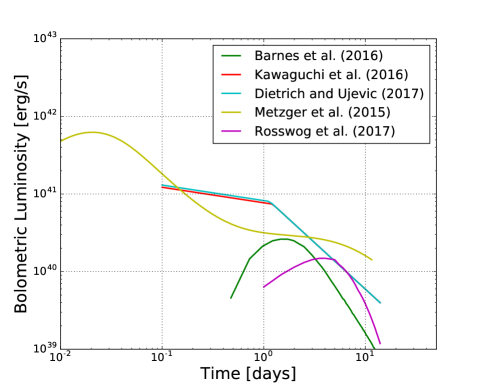
As a first comparison between different models, we consider a spherical ejecta with $M_{\rm ej}\approx 5\times 10^{-3}$ and $v_{\rm ej}\approx 0.2$, see Barnes et al. (2016). Here and in the following, we will give $v_{\rm ej}$ in fractions of the speed of light and masses in fractions of the mass of the sun $M_{\odot}$. For the non-spherical parametrized models of Kawaguchi et al. (2016) and Dietrich & Ujevic (2017), we further assume $\theta=0.2$ rad. From Rosswog et al. (2017), we include a model with $M_{\rm ej}=0.0079$ and $v_{\rm ej}=0.12$, which is closest to our fiducial model.

Additionally, we include the approximant of Metzger et al. (2015), which focused on the blue transient produced at a time around merger, which uses a neutron mass cut $m_{\rm n}=10^{-4}$, opacity of $\kappa=30$ $\textrm{cm}^{2}\textrm{g}^{-1}$, and electron fraction $Y_{\rm e}=0.05$.

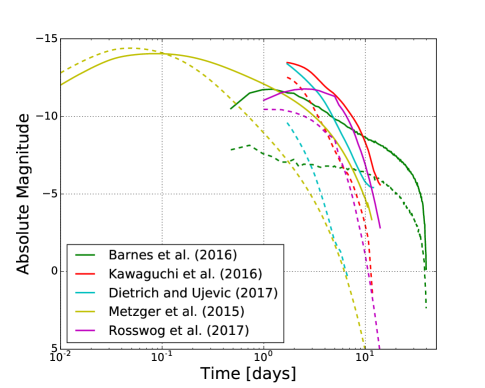
Figure 1 shows the bolometric luminosity and the lightcurves in the $g$- (dashed) and $i$- (solid) bands. The kilonovae models have significant short-term dynamics, with changes of more than a magnitude in less than a day. Both the Kawaguchi et al. (2016) and Dietrich & Ujevic (2017) models are based on the MC simulations of Tanaka et al. (2014) for which a constant thermal efficiency is assumed ($\epsilon_{\rm th}=0.5$).

The model of Barnes et al. (2016) includes a time dependent efficiency, which leads to a faster decay of the bolometric luminosity and magnitude because after a few days after the merger the thermalization efficiency drops below the constant thermalization efficiency employed in the Tanaka et al. (2014) simulations. Rosswog et al. (2017) employ both time dependent and constant efficiencies and use a more complex density profile. The model picked from Rosswog et al. (2017) shows a smaller bolometric luminosity than other models, notice, however, that as shown in Rosswog et al. (2017) the usage of different mass models effects the luminosity by about $\approx 600\%$, i.e., all presented models come with large uncertainties and crucially depent on nuclear physics assumptions. The model of Metzger et al. (2015) describes the blue transient arising from a small fraction of the ejected mass which expands sufficiently rapidly such that the neutrons are not captured and instead $\beta$-decay, giving rise to a clear peak in the bolometric luminosity visible around the time of merger.

Comparing Dietrich & Ujevic (2017) and Kawaguchi et al. (2016) we see a clear difference in the $g$-band. This has already been pointed out in Tanaka et al. (2014). The main difference seems to arise from the difference of employed bolometric corrections, which itself will depend on the ejecta morphology. Since BHNS ejecta are much more non-spherical and are concentrated in the equatorial plane, they have higher temperatures which make the spectrum bluer than BNS ejecta with the same mass.

Figure 2: Difference between the $g$- and $i$-bands for the models presented in Figure 1.

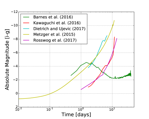
We can take the opportunity of having a variety of kilonova models accessible to compare the lightcurve colors. It is common in dedicated searches for kilonovae to make color cuts (Doctor et al., 2017). Figure 2 shows the difference between the $g$- and $i$-bands for the models presented in Figure 1. As expected, all of the kilonova models show differences of at least 2 mag, especially on later time scales. For this reason, independent of the employed kilonova model, the proposed analysis will optimize the strategy for the detection of GW optical counterparts. Given the relative consistency in color among the models, imaging the transients in both the blue/green and the near-infrared can help differentiate from other transients. Due to the high opacities of r-process nuclei, most models predict emission in the near infrared wavelengths. These observations are required within the first few days due to the faint magnitudes involved. As explained above, the significant changes in magnitude over day time-scales can also help differentiate them as compared to possible background transients such as SN Ia.

3.3 Dependence of the bolometric lightcurve on the density profile, morphology, and thermal efficiency

Figure 3: The comparison of the bolometric luminosity for various setups: The purple line employs a $\rho\propto r^{-2}$ density profile, spherical geometry, and a constant thermalization efficiency ($\epsilon_{\rm th}\approx 0.5$). The green line is similar to the purple curve but with non-spherical ejecta with $\theta_{\rm ej}=0.2$ and $\varphi=\pi$ [the same morphology employed in Kawaguchi et al. (2016), Dietrich & Ujevic (2017), and Barnes et al. (2016)]. The blue curve is similar to the purple curve but with $\rho\propto r^{-1}$ density profile. The orange line is similar to the blue one but with time-(mass)-dependent thermalization efficiency of Barnes et al. (2016). The yellow curve is similar to the blue curve but we employed a constant thermalization efficiency ($\epsilon_{\rm th}=1$) and multiplied afterwards by the time-(mass)-dependent thermalization efficiency given in Barnes et al. (2016). The red curve denotes the bolometric lightcurve employing $M_{\rm ej}=0.0079$ and $v_{\rm ej}=0.12$, and the same density profile as in Rosswog et al. (2017).

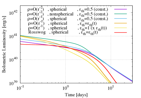
As shown in Figure 1 (left panel), the bolometric luminosity of the models from Kawaguchi et al. (2016), Dietrich & Ujevic (2017), Barnes et al. (2016), and Rosswog et al. (2017) can be significantly different (we do not include the blue transient proposed in Metzger et al. (2015) in the following analysis since it is powered by a different mechanism). While similar ejecta masses, velocities, and energy deposition rates are employed, the models use different density profiles, morphology, and thermalization efficiency. The models of Kawaguchi et al. (2016) and Dietrich & Ujevic (2017) assume $\rho\propto r^{-2}$ for the density profile, non-spherical geometry, and a constant thermalization efficiency ($\epsilon_{\rm th}\approx 0.5$). The model of Barnes et al. (2016) assumes spherical ejecta with $\rho\propto r^{-1}$ for the density profile and the time-(mass)-dependent thermalization efficiency is taken into account. The model of Rosswog et al. (2017) also assumes spherical ejecta with an homogeneously expanding density profile and time-(mass)-dependent thermalization efficiency with the FRDM model.

To check how these differences affect the bolometric lightcurves, we perform a simple radiation transfer simulation varying the density profile, ejecta morphology, and thermalization efficiency. In this calculation, we assume the flux limited diffusion approximation of the radiative transfer (Levermore & Pomraning, 1981), a constant gray opacity with $10\,{\rm cm^{2}g^{-1}}$, and the heating rate that is employed in Kawaguchi et al. (2016) and Dietrich & Ujevic (2017).

Figure 3 compares the bolometric luminosity for various setups. The figure clearly shows that different ejecta morphologies and thermalization efficiencies change the bolometric luminosity by about a factor of $\approx 2$. This explains qualitatively the difference in the bolometric luminosity and lightcurves in Figure 1. The difference in the model of Rosswog et al. (2017) is also explained by the difference in the ejecta mass, ejecta velocity, and thermalization efficiencies. On the other hand, a different density profile has only a minor effect.

These results indicate that for future development of analytical kilonovae approximants the focus should be put on modeling the ejecta morphology and the time-dependent thermalization efficiency. We also find that considering a constant thermalization efficiency of $\epsilon_{\rm th}=1$ and then multiplying with $\epsilon_{\rm th}(t)$ (given in Barnes et al. (2016)) or directly employing a time dependent thermal efficiency leads only to differences of $\approx 40\%$. This suggests that, at least for the bolometric luminosity, the time-dependency of the thermalization efficiency can be approximately taken into account just by multiplying its function to the luminosity obtained by the constant efficiency. This is of particular importance for further improvement of the parametrized models which, at the current stage, are based on simulations employing a constant thermalization efficiency.

In addition to the discussed effects further uncertainties exist, which make a modeling and prediction of kilonovae luminosities difficult. Rosswog et al. (2017) point out that the electron fraction and heating rate are main uncertainties in the current modeling of kilonovae lightcurves. They find that by using two different mass models (Duflo & Zuker (1995) (DZ31) and Finite Range Droplet Model (Moller et al., 1995)) the bolometric luminosity can be different up to $\approx 600\%$. This is caused by the fact that the nuclear heating rate enters linearly into the bolometric luminosity.

4 Model Comparisons and Parameter Estimation

In this section, we perform parameter estimation and model comparisons. We will use the Kawaguchi et al. (2016) and Dietrich & Ujevic (2017) models to compare both to other models and against themselves. As described, there are two parts to each of these models: the ejecta fitting formulas and the kilonovae lightcurves. Avoiding the ejecta fitting formulas, we can improve efficiency and accuracy by directly sampling the ejecta mass $M_{\rm ej}$ and velocity $v_{\rm ej}$, and later employ the correlations between the ejecta mass properties, e.g. ejecta mass $M_{\rm ej}$ and velocity $v_{\rm ej}$, and the binary parameters (see Section 5). Furthermore, we sample over the latitudinal and longitudinal opening angles, denoted as $\theta_{\rm ej}$ and $\phi_{\rm ej}$, respectively. Opacity, $\kappa=10$ $\textrm{cm}^{2}\textrm{g}^{-1}$, heating rate coefficient $\epsilon_{0}=1.58\times 10^{10}$ erg g^-1 s^-1, heating rate $\alpha=1.2$, and thermalization efficiency $\epsilon_{\rm th}=0.5$ are held fixed.

In this analysis, we will use a version of Multinest (Feroz et al., 2009b) commonly used in GW data analysis (Feroz et al., 2009a), and wrapped in python (Buchner et al., 2014). This algorithm has the benefit of computing the Bayesian evidence for a given set of parameters, which can be used to assign relative probabilities to different models. The likelihood evaluation proceeds as follows. For each parameter set sampled, lightcurves in $griz$ bands are computed. We use linear extrapolation of the magnitudes to extend the lightcurves in cases where the model does not predict the full time covered by the target lightcurve. In addition to the parameters above, we also allow the lightcurves to shift in time by an offset $T_{0}$, which allows for a measurement of the initial time of the kilonovae and therefore gives important evidence for a potential counterpart, and in magnitude by a color-independent zeropoint offset ZP, which compensates for our ignorance about the distance to the source. A $\chi^{2}$ distribution is then calculated between the lightcurve produced from the model and the target lightcurve. The likelihood is then simply that from a $\chi^{2}$ distribution. The priors used in the analyses are as follows: $-5\leq T_{0}\leq 5$ days, $-50.0\leq\textrm{ZP}\leq 50.0$ mag, $-5\leq\log_{10}(M_{\rm ej})\leq 0$, $0\leq v_{\rm ej}\leq 1$, $0\leq\theta\leq\pi/2$ rad, and $0\leq\phi\leq 2\pi$ rad. The priors are flat over the stated ranges.

4.1 Self-consistency check of parametrized models

Figure 4: The top row shows lightcurves for Dietrich & Ujevic (2017) (left) and Kawaguchi et al. (2016) (right). We use lightcurves with $M_{\rm ej}=5\times 10^{-3}$, $v_{\rm ej}=0.2$, $\theta_{\rm ej}=0.2$ rad, and $\phi_{\rm ej}=3.14$ rad for the lightcurve computation. We also perform a maximum likelihood $\chi^{2}$ fit to each lightcurve using the same models for comparison. The lines with error bars show the injected lightcurve with the assumed 1 mag error budget. The dashed black lines show the best fit lightcurve to that model, including the linear extrapolation. The bottom row shows the corresponding corner plots.

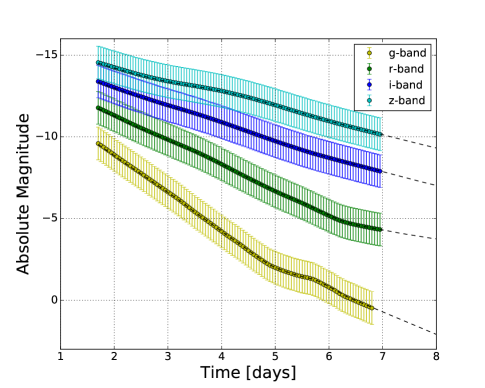
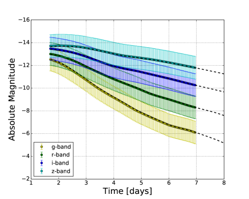
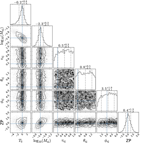
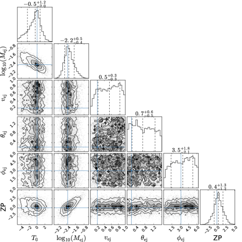
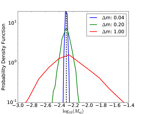
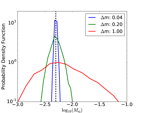
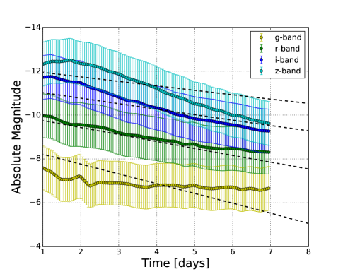
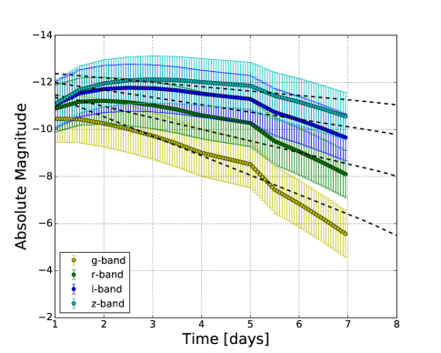
As a first test of the numerical method, we use lightcurves produced by the parametrized models for BNS and BHNS and also recover the ejecta properties with the same models. The top row of Figure 4 shows lightcurves of such a comparison, where we assume uncertainties of the models of 1 mag as stated in Dietrich & Ujevic (2017) and Kawaguchi et al. (2016). The top row shows that the injected lightcurves are recovered properly. We quantify the level of overlap between parameters with “corner” plots (Foreman-Mackey, 2016), shown in the bottom row of Figure 4. Shown are 1- and 2-D posteriors marginalized over the rest of the parameters. In general, there are a few key features. First, with the $\approx 1$ mag uncertainty associated to these models, a large number of lightcurves computed with the parametrized models are consistent with the injected/baseline lightcurve we took. This means that no strict parameter constraints can be obtained. But, although the models have stated $\approx 1$ mag uncertainty, we can study a possible scenario with models having smaller uncertainties, e.g. $\approx 0.2$ mag or even $0.04$ mag, which approximate the characteristic uncertainty for observations. In Figure 5, we show histograms for $M_{\rm ej}$ for the case where the uncertainties are varied. The figure demonstrates that $M_{\rm ej}$ constraints are significantly improved when the assigned error to the model is small. In particular for an uncertainty of $0.2$ mag the ejecta mass can be determined up to $\log_{10}M_{\rm ej}\approx\pm 0.5$, and in cases where the uncertainty would be limited by the observation (uncertainty of $0.04$ mag) the ejecta mass could be determined to $\log_{10}M_{\rm ej}\approx\pm 0.1$. This motivates the need for further improved parametrized models of kilonovae lightcurves.

In contrast to the ejecta mass, the ejecta velocity is poorly constrained in our analysis. This is because the analytic models do not include times $t\lesssim 1\,{\rm day}$, where the ejecta are optically thick. However, the dependence on the ejecta velocity is only significant during this stage. Afterwards, the lightcurves is primarily determined by the ejecta mass. Therefore, to improve the estimation of the ejecta velocity, extension of the lightcurve models to earlier times is required.

Figure 5: Histograms of $M_{\rm ej}$ recovery. We inject lightcurves computed with the parametrized model of Dietrich & Ujevic (2017) (left) and Kawaguchi et al. (2016) (right). We recover the injected lightcurve with the same model. For decreasing uncertainties assigned to the models, the ejecta mass gets better constrained and approaches the true value (vertical dash-dotted).

4.2 Comparison with Tanaka et al.

Figure 6: Histograms of $M_{\rm ej}$ for the BNS and BNHS lightcurves from Tanaka et al. (2014) compared with the Dietrich & Ujevic (2017) model (left) and Kawaguchi et al. (2016) model (right), respectively. For this analysis, there are errors of 0.2 mag (solid lines) and errors of 1 mag (dash-dotted lines).

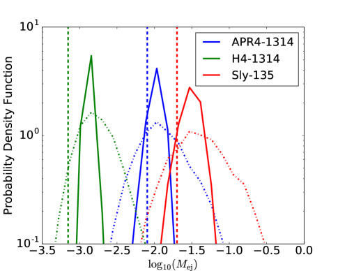
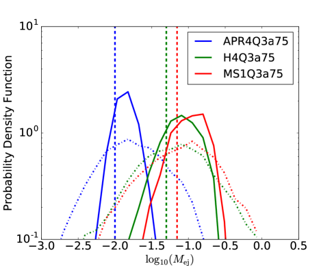
We now perform a comparison between the parameterized models and results from Tanaka et al. (2014). For this analysis, we distinguish between BNS and BHNS. The BNS setups of Tanaka et al. (2014) are compared to the Dietrich & Ujevic (2017) model and the BHNS lightcurves are compared to the Kawaguchi et al. (2016) model. In Figure 6, we show histograms for $M_{\rm ej}$ for uncertainties of 1 mag (dash-dotted lines), which corresponds to the error stated in Kawaguchi et al. (2016) and Dietrich & Ujevic (2017). The ejecta mass corresponding to the lightcurves of Tanaka et al. (2014) (vertical dashed lines) is always within the posteriors of the models for the 1 mag posteriors (dash-dotted). We find that for 0.2 mag (solid lines) uncertainties some of the true values for BNS systems lie outside the estimated posteriors, which is to be expected because the uncertainties in Dietrich & Ujevic (2017) and Kawaguchi et al. (2016) are 1 mag. But, even for an assigned uncertainty of 0.2 mag, the posteriors of the BHNS setups are consistent with the injected values, which suggests that recovering smaller ejecta masses is in general less accurate. This might be caused by inaccuracies in the employed bolometric corrections and is already visible in Figure 9 of Dietrich & Ujevic (2017).

4.3 Comparison with other kilonova models

Figure 7: Lightcurves for Barnes et al. (2016) (top) and Rosswog et al. (2017) (bottom) with the same parameters as from Figure 1. We also perform a maximum likelihood chi-squared fit to each lightcurve using the Dietrich & Ujevic (2017) model for comparison.

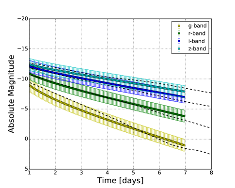
We now perform a comparison between the parametric models and Barnes et al. (2016); Rosswog et al. (2017). In Figure 7, we take the Barnes et al. (2016) (top panel) model rpft_m005_v2 and the NS14B7 model of Rosswog et al. (2017) (bottom panel), and use the Dietrich & Ujevic (2017) model for recovery. One finds that the relative magnitudes between the bands is mostly consistent across the models. However, the models are not able to reproduce the lightcurves as accurately as for Tanaka et al. (2014). We find that multiple parameters, including the ejecta mass, cannot be constrained. Furthermore, for Rosswog et al. (2017) the parameter estimation pipeline leads to a $T_{0}$ estimate of the order of a few days, which suggests that follow up searches using the current parametrized models would not correctly detect transients with lightcurves similar to those given in Rosswog et al. (2017).

The origin of the difference between the parameterized models and Barnes et al. (2016); Rosswog et al. (2017) is that Dietrich & Ujevic (2017) was built using the lightcurves of Tanaka et al. (2014). It can be expected that parametrized models approximating the results of Barnes et al. (2016) and Rosswog et al. (2017) can be obtained as well. This shows that for future development, it is urgently required to provide lightcurves using full radiative transfer simulations that are as realistic as possible, i.e. including different ejecta components, time dependent efficiency, and complex ejecta morphologies.

4.4 Comparison with other models

Figure 8: Lightcurves for Metzger et al. (2015) (top), with the same parameters as from Figure 1, and a SN Ia from Guy et al. (2007) (bottom). We also perform a maximum likelihood chi-squared fit to each lightcurve using the Dietrich & Ujevic (2017) model for comparison.

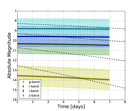
We also compare to a few non-kilonova models in Figure 8. Considering the different origin of the EM signal, we expect that the kilonova models cannot capture the injected lightcurves. We use the Metzger et al. (2015) fiducial model (top panel of Figure 8) describing the blue kilonovae precursor and a SN Ia model from Guy et al. (2007) (bottom panel). Metzger et al. (2015) does have an initially higher blue component. The best fit curve from Dietrich & Ujevic (2017) is capable of producing time dependent lightcurve approximants. For the SN Ia it was not possible to compute time dependent lightcurves with the parametrized models which approximate the SN Ia lightcurve. This shows that the parametrized models can also help to distinguish transients with different origins.

5 Extracting the binary parameters

Our previous study focused on the question how we can use parametrized models to obtain information about the mass, velocity, and morphology of the ejecta. At least as important for astrophysical considerations is the question whether measured lightcurves can be used to directly constrain the binary properties: masses, spins, and possibly also the unknown EOS. To achieve this goal, phenomenological models connecting the ejecta properties as well as the binary parameters have to be employed. Such models based on large sets of NR simulations are given in Kawaguchi et al. (2016) for BHNS systems and in Dietrich & Ujevic (2017) for BNS systems. Because of the large uncertainties in the determination of the ejecta mass in full general relativistic simulations, current parametrized models can only be seen as a starting point to more accurate models. Longer simulations with detailed microphysics are needed to properly model all the ejecta components.

5.1 Possible Degeneracies

Figure 9: Binary parameters of a BHNS systems, Equation 5.1 and Equation 2, which lead to $M_{\rm ej}=10^{-2}$ (red surfaces) and $v_{\rm ej}=0.28$ (blue surface) under the assumption of different compactnesses $C=0.13,0.15,0.17$ (from left to right). Because of the degeneracies between the binary parameters and the ejecta properties an unambiguous measurement of $q,M_{\rm NS}^{*},\chi_{\rm eff},C$ is not possible if only $M_{\rm ej}$ and $v_{\rm ej}$ are measured.

In addition to the large uncertainty of the NR data, the models also contain degeneracies which do not allow the simultaneous extraction of all binary parameters. The ejecta mass and velocity as functions of the binary parameters for BHNS can be approximated by:

$$\frac{M_{\rm ej}}{M_{\rm NS,*}} = {\rm Max}\left\{a_{1}q^{n_{1}}\frac{1-2C}{C}-a_{2}\,q^{n_{2}}\,{\tilde{r}}_{\rm ISCO}(\chi_{\rm eff})\right.$$

$$+ \left.a_{3}\left(1-\frac{M_{\rm NS}}{M^{*}_{\rm NS}}\right)+a_{4},0\right\},$$

$$v_{\rm ej} = b_{1}\,q+b_{2}.$$ (2)

with $\chi_{\rm eff}=\chi\,{\rm cos}\,i_{\rm tilt}$, where $i_{\rm tilt}$ is the angle between the dimensionless spin of the black hole $\chi$ and the orbital angular momentum and ${\tilde{r}}_{\rm ISCO}$ is the radius of the innermost stable circular orbit normalized by the black hole mass. $a_{1},a_{2},a_{3},a_{4},n_{1},n_{2},b_{1},b_{2}$ are fitting parameters which are determined by comparison to a large set of NR data, see Kawaguchi et al. (2016). For BNS setups, the ejecta properties are approximated by

$$M_{\rm ej}^{\rm fit} = 10^{-3}\left[\left\{a\left(\frac{M_{2}}{M_{1}}\right)^{1/3}\left(\frac{1-2C_{1}}{C_{1}}\right)+b\left(\frac{M_{2}}{M_{1}}\right)^{n}\right.\right.$$

$$+ \left.\left.c\left(1-\frac{M_{1}}{M^{*}_{1}}\right)\right\}M_{1}^{*}+(1\leftrightarrow 2)+d\right],$$

$$v_{\rm ej} = \sqrt{v_{\rho}^{2}+v_{z}^{2}},$$ (4)

$$v_{\rho,z} = \left[a_{\rho,z}\left(\frac{M_{1}}{M_{2}}\right)\left(1+c_{\rho,z}\ C_{1}\right)\right]+(1\leftrightarrow 2)+b_{\rho,z},$$ (5)

$$\theta_{\rm ej} = \frac{2^{4/3}v_{\rho}^{2}-2^{2/3}(v_{\rho}^{2}(3v_{z}+\sqrt{9v_{z}^{2}+4v_{\rho}^{2}}))^{2/3}}{(v_{\rho}^{5}(3v_{z}+\sqrt{9v_{z}^{2}+4v_{\rho}^{2}}))^{1/3}},\quad$$ (6)

$$\phi_{\rm ej} = 4\theta_{\rm ej}+\frac{\pi}{2},$$ (7)

with the fitting parameters $a,b,c,d,a_{\rho},a_{z},b_{\rho},b_{z},c_{\rho},c_{z},n$ given in Dietrich & Ujevic (2017).

As can be concluded from the Equations 5.1-7, the BHNS model depends on: the mass ratio $q$, the “effective” spin of the black hole $\chi_{\rm eff}$, the baryonic mass of the neutron star $M_{\rm NS}^{*}$, the quotient of the neutron star’s gravitational mass $M_{\rm NS}$ and baryonic mass $M^{*}_{\rm NS}$, and its compactness $C$, i.e., five parameters. For the case of BNS systems, the number increases to six: the gravitational masses $M_{1},M_{2}$, the baryonic masses $M_{1}^{*},M_{2}^{*}$, and the compactnesses $C_{1},C_{2}$ of the neutron stars.

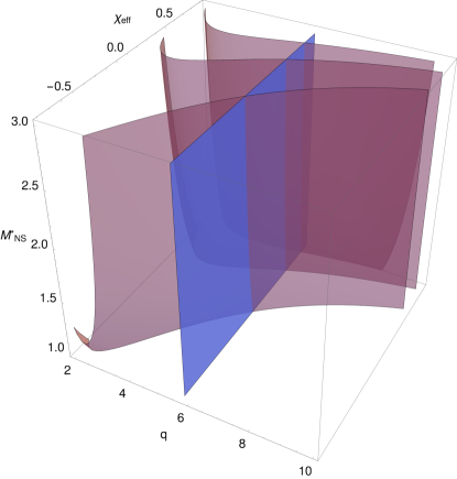
As an example to visualize possible degeneracies in Equations 5.1-7, let us suppose that the ejecta mass and the ejecta velocity was measured for a BHNS setup. In Figure 9, we show as red surfaces the allowed binary parameters for which $M_{\rm ej}=10^{-2}$ under the assumptions of $C=0.13,0.15,0.17$. In addition, we make use of the quasi-universal relation Equation 8 to connect the gravitational and baryonic mass to the compactness, see discussion in the next subsection. As a blue surface, we mark the binary parameters for which $v_{\rm ej}=0.28$. According to Equation 2, the measurement of $v_{\rm ej}$ would determine the mass ratio of the system $q$ but leave the other parameters unconstrained.

Figure 9 shows that even if $M_{\rm ej}$ and $v_{\rm ej}$ are accurately known, the binary parameters cannot be determined. The intersections between the red and blue surfaces mark all the allowed regions for which the ejecta properties are consistent with the estimated $M_{\rm ej},v_{\rm ej}$ under the assumption of a given compactness $C$. Consequently, an accurate measurement of the binary properties is only possible for cases for which more parameters than $M_{\rm ej},v_{\rm ej}$ are determined, e.g. $\theta_{\rm ej}$ and $\phi_{\rm ej}$, or for cases where due to a simultaneous detection of GWs some binary parameters are known.

5.2 Quasi-universal properties

Figure 10: Ratio of the baryonic mass and gravitational mass $M^{*}/M$ as a function of the compactness for different equations of state (top panel) and difference for $M^{*}/M$ between each EOS and the approximant Equation (8) (bottom panel). The dashed black line corresponds to the fit.

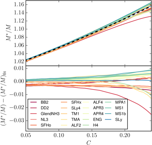
Due to the large number of unknown binary parameters in Equations 5.1-7, several degeneracies exist and binary parameters cannot be constrained uniquely. To reduce this effect, we substitute some parameters with the help of quasi-universal relations. Quasi-universal properties for single neutron stars have been first found by Yagi & Yunes (2013) and were consequently studied for a variety of parameters, see e.g. Maselli et al. (2013); Pappas & Apostolatos (2014); Yagi et al. (2014); even in BNS systems quasi-universal relations are present, e.g. Bernuzzi et al. (2014). We propose a relation between the quotient of baryonic and gravitational mass $M^{*}/M$ and the compactness $C$ of a single neutron star. To construct this relation, we use the EOSs employed for the dataset studied in Dietrich & Ujevic (2017), but only consider EOSs which allow non-rotating NS masses above $1.9$, which lies even below the highest measured NS mass of $\approx 2.01$. Figure 10 shows $M^{*}/M$ as a function of the compactness $C$ for all EOSs. We find that only a small spread is caused by the EOSs. Except for GlendNH3, all curves stay close together.

We fit all data with an approximant of the form

$$\frac{M^{*}}{M}=1+a~{}C^{n},$$ (8)

the free fitting parameters are $a=0.8858$ and $n=1.2082$. The fit is included as a black dashed line in the top panel of Figure 10. By construction, we obtain for $C\rightarrow 0$ the correct limit of $M^{*}/M\rightarrow 1$. The residuals of the fit is shown in the bottom panel of Figure 10. Absolute errors within the compactness interval of $C\in[0.05,0.24]$ are within $\pm 0.01$, except for GlendNH3. This leads to fractional errors of $\lesssim 10\%$ for the term $1-M^{*}/M$ which enters directly in the ejecta mass computation for BHNS and BNS systems. On average fractional errors are $\lesssim 3\%$. Considering the large uncertainty of Equations 5.1-7, we expect that the error caused by Equation (8) is negligible. But by introducing this relation, the number of free parameters for the BHNS model is reduced by one and for the BNS model reduced by two. This allows for significantly better extraction of the binary parameters from the ejecta properties.

5.3 Extraction of binary parameters

Figure 11: On the left is the corner plot for the model fits for the Dietrich & Ujevic (2017) model with $M_{\rm ej}=5\times 10^{-3}$, $v_{\rm ej}=0.25$ and an optimistic 1% Gaussian errorbar on the measurement. On the right is the same for the Kawaguchi et al. (2016) model with $M_{\rm ej}=5\times 10^{-2}$ and $v_{\rm ej}=0.25$ for comparison with the same error bars.

In the following, we use a similar scheme as in Sec. 4 to explore how binary parameters can be recovered from a kilonovae detection. We explore the situation where we have made a measurement of $M_{\rm ej}$ and $v_{\rm ej}$. We calculate the likelihood using a kernel density estimator commonly used in GW data analysis (Singer et al., 2014). This technique is useful for cases where the measurements of those distributions arise from parameter estimation with potentially highly correlated estimates amongst the variables, as is common in GW data analysis. The priors used in the analyses are as follows: For Kawaguchi et al. (2016), $3\leq q\leq 9$, $0\leq\chi_{\rm eff}\leq 0.75$, $1\leq M_{\rm NS}\leq 3$, and $0.1\leq C\leq 0.2$, while for Dietrich & Ujevic (2017), $1\leq M_{1}\leq 3$, $1\leq M_{2}\leq 3$, $0.08\leq C_{1}\leq 0.24$, and $0.08\leq C_{2}\leq 0.24$. The differences in compactness prior ranges are due to the differences in compactness used in the simulations the models used. The priors are flat over the stated ranges. For this reason, significant structure in the 1D and 2D contours arise from the posterior.

To begin, we explore the correlation between the variables by employing the very optimistic assumption of 1% Gaussian errorbars on the measurement, which essentially inverts the equations in the previous section. We show in Figure 11 the parameters consistent with two different choices of $M_{\rm ej}$ and $v_{\rm ej}$. For the BNS case (left panel), we choose $M_{\rm ej}=5\times 10^{-3}$ and $v_{\rm ej}=0.25$, for the BHNS case (right panel), we choose $M_{\rm ej}=5\times 10^{-2}$ and $v_{\rm ej}=0.25$. In general, for the BNS systems, the constraints are not strong given the relatively wide variety of parameters that support non-zero ejecta masses and velocities. We choose to plot mass ratio ($q=M_{1}/M_{2}$) and chirp mass [$M_{\rm c}=(M_{1}M_{2})^{3/5}(M_{1}+M_{2})^{-1/5}$] instead of $M_{1}$ and $M_{2}$, due to the clearer peaks in this parameterization. We clearly see in the 2D corner plots degeneracies between $M_{\rm c}$ and $q$ as well as between $C_{1}$ and $C_{2}$, which are similar to those described in the previous subsection. These indicate the fundamental limitations of EM-only observations in the measurements of these quantities. For the BHNS systems, the main constraint is on $q$, which has some correlation with compactness. Due to the significant correlations between $q$, $\chi_{\rm eff}$, and $C$, it will be difficult to constrain those parameters without measurements from other quantities.

Figure 12: On the left is the corner plot for the model fits for the Dietrich & Ujevic (2017) model for $M_{\rm ej}$ and $v_{\rm ej}$ contours sampled from a lightcurve with $M_{\rm ej}\approx 5\times 10^{-3}$, $v_{\rm ej}\approx 0.2$ (similar to Figure 11) and model uncertainties of $0.2$ mag. On the right is the same for the Kawaguchi et al. (2016) model for comparison.

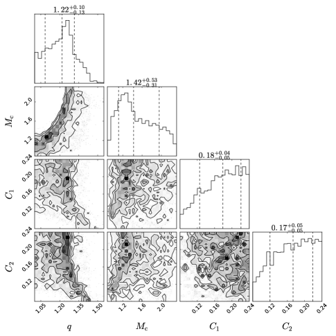
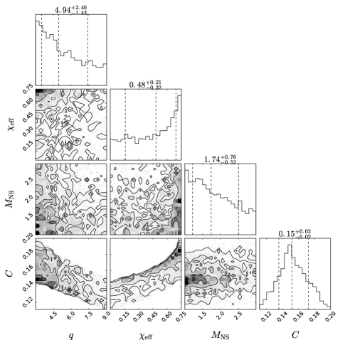
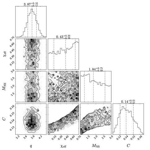
Figure 12 shows more realistic levels of parameter estimates using the $M_{\rm ej}$ and $v_{\rm ej}$ contours sampled from a lightcurve with $M_{\rm ej}\approx 5\times 10^{-3}$ and $v_{\rm ej}\approx 0.2$ with model uncertainties of $0.2$ mag. The main difference in these results and the optimistic assumptions above is the relatively poor constraints on $v_{\rm ej}$. For the BNS system (left panel), because the constraints on mass ratio are tied to $v_{\rm ej}$, most values of mass ratio are allowed in this particular case. There are only minimal constraints on $M_{\rm c}$, $C_{1}$, and $C_{2}$. For the BHNS system (right panel), the only structure visible is the correlation between $q$, $\chi_{\rm eff}$, and $C$. In case of precise measurement of the mass ratio and effective spin by GW parameter estimation, constraints on the neutron star compactness of $C\pm 0.2$ is possible.

Figure 13: Corner plots for lightcurves with $M_{\rm ej}=5\times 10^{-3}$ $v_{\rm ej}=0.2$, $\theta_{\rm ej}=0.2$ rad, and $\phi_{\rm ej}=3.14$ rad using the Dietrich & Ujevic (2017) model with 0.2 mag uncertainty.

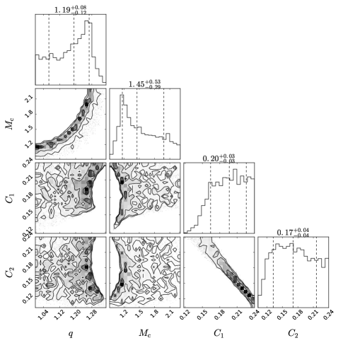
As a final comparison, we perform parameter estimation for the Dietrich & Ujevic (2017) model with 0.2 mag uncertainty, but instead of sampling in $M_{\rm ej}$ and $v_{\rm ej}$, we sample directly in the system parameters making use of Equations 5.1-7. Figure 13 shows the corner plots for this scenario. We find that the individual binary parameters are almost undetermined, only in the 2D $M_{1}$-$M_{2}$ or, as shown in the figure, $M_{\rm c}$-$q$ plane a clear contour is visible. According to the 1D posteriors of $q$ it seems that high mass ratios are ruled out. Additionally, $C_{1},C_{2}$ are almost unconstrained, but there seems to be a small preference for larger compactnesses for the shown example.

Although we have only discussed the extraction of binary parameters for BNS configurations similar results are obtained for BHNS systems.

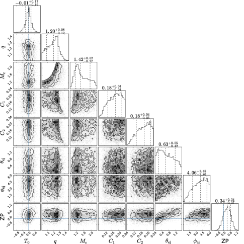
6 Synergy of electromagnetic and gravitational wave observations

Figure 14: Histograms of $M_{\rm ej}$ (top left), $v_{\rm ej}$ (top right), $M_{\rm c}$ (bottom left), and $q$ (bottom right) for EM-only, GW-only and combined EM-GW constraints on a simulated BNS with GW parameter estimation from Singer et al. (2014). Parameter estimation using a simulated lightcurve from the Dietrich & Ujevic (2017) model consistent with this simulated BNS was used to generate the EM constraints. For this analysis we assume 0.2 mag (solid lines) and 1 mag (dash-dotted lines) uncertainties of the kilonova model. The injected (true) value is marked as a vertical dashed line. In the case of $M_{\rm c}$, the GW-only line lies directly below the GW-EM line.

As described in the previous section, the constraints on $M_{\rm c}$ and $q$ from EM observations alone are limited. On the other hand, GW parameter estimation provides direct constraints on these quantities as well. In particular, $M_{\rm c}$ is strongly constrained (Abbott et al., 2016a, b, 2017). Previously, the idea of using EM transients as triggers in searches for GWs from compact binary mergers was proposed (Kelley et al., 2013). Also, the possibility of combining host galaxy identification with GW parameter estimation to yield improved constraints on binary inclination have been mentioned before (Fan et al., 2014). Additionally, we can use information from the GW parameter estimation combined with constraints from the EM parameter estimation to improve limits on the ejecta properties.

To demonstrate the benefits of this kind, we take an example from Singer et al. (2014), which includes both GW skymaps and posteriors from the parameter estimation of BNS signals. We take one such example and generate a lightcurve using the Dietrich & Ujevic (2017) model corresponding to the mean of the mass posteriors with compactnesses of $C_{1,2}=0.147$, and use the quasi-universal relation, Equation 8, to compute the baryonic masses. The true values are $M_{\rm ej}=0.006$ and $v_{\rm ej}=0.2$. We use magnitude uncertainties of 1.0 mag and 0.2 mag.

We perform the same parameter estimation technique as in the previous sections to derive EM-only constraints on $M_{\rm ej}$ and $v_{\rm ej}$. We then use the GW parameter estimation posteriors of $M_{1}$ and $M_{2}$ to derive GW-only constraints on $M_{\rm ej}$ and $v_{\rm ej}$. This is accomplished by using a kernel density estimator on the GW posteriors of $M_{1}$ and $M_{2}$ and allowing $C_{1}$ and $C_{2}$ to vary using the same priors as with the EM parameter estimation. Combining these posteriors is performed straightforwardly by multiplying the probabilities derived from both the GW-only and the EM-only posteriors, but note that because we are multiplying 2-D probabilities from correlated variables, the marginalized posteriors from the combined analysis can look different from multiplying the 1-D marginalized distributions.

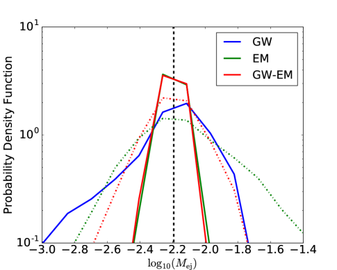
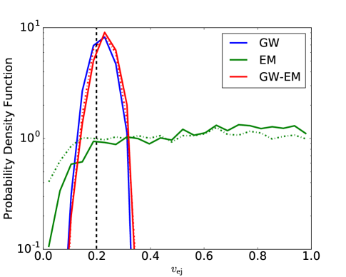
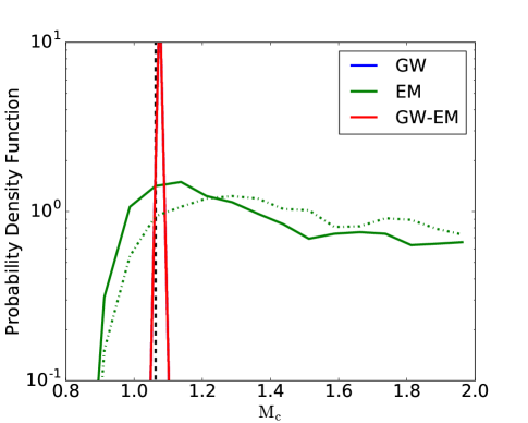
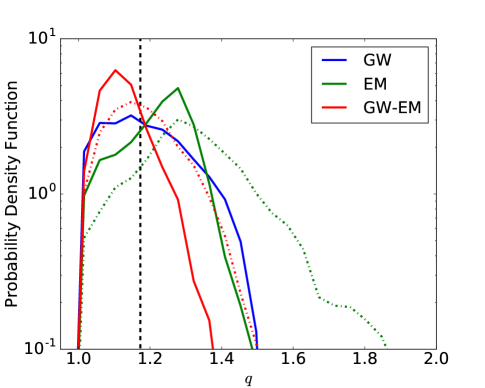
In Figure 14, we show histograms for $M_{\rm ej}$, $v_{\rm ej}$, ${\rm M}_{\rm c}$, and $q$ for EM-only (green), GW-only (blue) and combined EM-GW (red) constraints. The figure demonstrates that significant improvements are possible with joint EM- and GW-parameter estimation. For example, whereas there are almost no limits on $v_{\rm ej}$ with EM-only, constraints from GW parameter estimation create a clear peak in the posterior and the ejecta velocity can be determined up to $v_{\rm ej}\approx\pm 0.15$. The limits on $M_{\rm ej}$ show the true synergy between potential EM and GW parameter estimation. The broad posteriors of the EM-only and GW-only are narrowed when combined, e.g., for an uncertainty of 1.0 mag the uncertainty decreases from $\log_{10}M_{\rm ej}\approx\pm 0.75$ to $\log_{10}M_{\rm ej}\approx\pm 0.4$. In the case where a magnitude uncertainty of 0.2 mag is employed, the constraints on velocity are still dominated by the GW parameter estimation, but the $M_{\rm ej}$ determination is dominated from the EM measurement.

Considering the binary parameters, we find that for 0.2 mag and 1.0 mag the chirp mass $M_{\rm c}$ is purely constrained by the GW parameter estimation. On the other hand, while for a magnitude uncertainty of 1 mag, the mass ratio is mostly determined by GW parameter estimation with only minor improvement once EM parameter estimation is also considered, one finds that for magnitude uncertainty of 0.2 mag, constraints are improved and decrease from $q\approx\pm 0.25$ to $q\approx\pm 0.2$. Due to the minimal correlation between $M_{\rm c}$, $q$ and the compactnesses, improved constraints on the compactnesses is not expected.
It is important to note that there is no bias in the measurement of $q$ in the GW-EM case. The 1-D posterior for $q$ shifts left as the EM error bars are reduced due to the significant correlation between $M_{\rm c}$ and $q$ from the parameter estimation, as can be seen from the left of Figure 12.

In summary, $M_{\rm c}$ and $v_{\rm ej}$ can be constrained by GW parameter estimation, with little improvement from the inclusion of EM results. On the other hand, with the uncertainty budgets of current kilonova models and relations between binary parameters and ejecta properties, combined GW-EM parameter estimation improves possible constraints for both $M_{\rm ej}$ and $q$. While it is true that in a future where kilonova models have improved such that their uncertainties are at the order of observation level, the EM observations will dominate the $M_{\rm ej}$ and $q$ constraints and therefore a combined analysis would not be useful, however, it is unlikely that such big improvements can be made in the near future. This motivates the importance for coordination between GW and EM parameter estimation in the event of a kilonova counterpart detection.

7 Conclusion

In this article, we compared different lightcurve models, outlined differences and similarities, and checked the consistency amongst the models. We showed how parameter estimation based on the kilonovae lightcurves depends on the uncertainty of the employed models.

We found that the parametrized models of Kawaguchi et al. (2016) and Dietrich & Ujevic (2017) are able to recover the lightcurves and parameters of the radiative transfer simulations of Tanaka et al. (2014). As we have shown in Figures 5 and 6, the ejecta properties can be determined accurately once the models have small uncertainty, e.g., an estimate of the ejecta mass of $\log_{10}M_{\rm ej}\approx\pm 0.5$ could be obtained once the model’s uncertainty is below $0.2\,$mag. We find that currently both the Kawaguchi et al. (2016) and Dietrich & Ujevic (2017) models are consistent with their stated uncertainties (and Kawaguchi et al. (2016) perhaps even better than that), and that there are significant gains in parameter estimation to be made when these uncertainties decrease. We hypothesize that for updated simulations using more detailed microphysical descriptions, in particular a better treatment of weak interaction, i.e. neutrino physics, it would also be possible to produce analytic models for the results of NR and radiative transfer simulations. With a model that both describes the improved simulations and has smaller inherent uncertainties in hand, it is in principle possible to make precision measurements of ejecta mass with results limited only by observation.

To improve the parameter estimation and allow for an extraction of the binary properties, we introduced a quasi-universal relations between the quotient of baryonic and gravitational mass $M^{*}/M$ and the compactness $C$ of a single neutron star. This relation reduced the number of free parameters for the parameter estimation and consequently improved the extraction of the individual binary parameters. We also compared the parametrized models with other kilonova models and lightcurves of other transients. As expected, the lightcurves of a blue kilonovae precursor and a SN Ia cannot be approximated by the models, which shows that the parametrized models could also be used to rule out some of the possible measured transients. We also found that other kilonovae lightcurves, Barnes et al. (2016) and Rosswog et al. (2017), are not accurately described as well. This is caused by the difference in the underlying radiative transfer simulations on which the models are built, which emphasizes again the need to improve and update kilonova models in the future.

We also showed how to include the posterior samples from GW signals from a binary-neutron star or black hole-neutron star to give further constraints on parameters for the lightcurves. We showed improved constraints on the ejecta properties $M_{\rm ej},v_{\rm ej}$ and the binary parameters $M_{\rm c},q$ using a combination of GW and EM observations. This motivates combined analysis in the case of a kilonovae detection coincident with a GW trigger.

However, a number of hurdles remain. Mostly due to the large uncertainties in the ejecta mass, velocity, density profile, the effect of thermal efficiency, and the estimated opacity in the ejected material, there are large biases and parameter estimation with the current existing models is hampered. To overcome these issues, improvements have to be made in numerical relativity by performing longer simulations which include additional physics such as other ejecta components from magnetic driven winds or neutrino outflows, see e.g. Surman et al. (2008); Metzger et al. (2008); Dessart et al. (2009); Perego et al. (2014). Additionally, improved radiative simulations will be needed. Based on those simulations, new parametrized models could be developed in the future.

For future application, it will also be useful to consider how to implement a search strategy in existing data sets when the lightcurves are not necessarily well sampled. This would optimize the tiling and time allocation strategies of existing searches for GW counterparts with telescopes with wide fields of view.

A code to produce the results in this paper is available at https://github.com/mcoughlin/gwemlightcurves for public download. Required for analysis are text files of lightcurves from models of interest in magnitudes, typically available from groups developing kilonova models. Furthermore, the kilonovae model of Kawaguchi et al. (2016) can be found online on www2.yukawa.kyoto-u.ac.jp/~kyohei.kawaguchi/kn_calc/main.html and the model of Dietrich & Ujevic (2017) on www.aei.mpg.de/~tdietrich/kn/main.html.

8 Acknowledgments

The authors would like to thank Zoheyr Doctor for a careful reading of an earlier version of the manuscript. MC is supported by National Science Foundation Graduate Research Fellowship Program, under NSF grant number DGE 1144152. CWS is grateful to the DOE Office of Science for their support under award DE-SC0007881. MU is supported by Fundação de Amparo à Pesquisa do Estado de São Paulo (FAPESP) under the process 2017/02139-7. KK is supported by JSPS Postdoctoral Fellowships for Research Abroad.

References

- Abbott et al. (2016a) Abbott, B. P., Abbott, R., Abbott, T. D., et al. 2016a, Phys. Rev. Lett., 116, 061102
- Abbott et al. (2016b) —. 2016b, Phys. Rev. Lett., 116, 241103
- Abbott et al. (2016c) —. 2016c, Astrophys. J., 826, L13
- Abbott et al. (2017) —. 2017, Phys. Rev. Lett., 118, 221101
- Barnes & Kasen (2013) Barnes, J., & Kasen, D. 2013, Astrophys. J., 775, 18
- Barnes et al. (2016) Barnes, J., Kasen, D., Wu, M.-R., & Martínez-Pinedo, G. 2016, Astrophys. J., 829, 110
- Bernuzzi et al. (2014) Bernuzzi, S., Nagar, A., Balmelli, S., Dietrich, T., & Ujevic, M. 2014, Phys. Rev. Lett., 112, 201101
- Berry et al. (2015) Berry, C. P. L., Mandel, I., Middleton, H., et al. 2015, Astrophys. J., 804, 114
- Buchner et al. (2014) Buchner, J., Georgakakis, A., Nandra, K., et al. 2014, Astron. Astrophys., 564, A125
- Cowperthwaite & Berger (2015) Cowperthwaite, P. S., & Berger, E. 2015, The Astrophysical Journal, 814, 25. http://stacks.iop.org/0004-637X/814/i=1/a=25
- Dessart et al. (2009) Dessart, L., Ott, C., Burrows, A., Rosswog, S., & Livne, E. 2009, Astrophys. J., 690, 1681
- Dietrich & Ujevic (2017) Dietrich, T., & Ujevic, M. 2017, Class. Quant. Grav., 34, 105014
- Doctor et al. (2017) Doctor, Z., Kessler, R., Chen, H. Y., et al. 2017, Astrophys. J., 837, 57
- Duflo & Zuker (1995) Duflo, J., & Zuker, A. P. 1995, Phys. Rev., C52, R23
- Fairhurst (2009) Fairhurst, S. 2009, New Journal of Physics, 11, 123006
- Fairhurst (2011) Fairhurst, S. 2011, Class. Quant. Grav., 28, 105021
- Fan et al. (2014) Fan, X., Messenger, C., & Heng, I. S. 2014, The Astrophysical Journal, 795, 43
- Feroz et al. (2009a) Feroz, F., Gair, J. R., Hobson, M. P., & Porter, E. K. 2009a, Class. Quant. Grav., 26, 215003
- Feroz et al. (2009b) Feroz, F., Hobson, M. P., & Bridges, M. 2009b, Mon. Not. Roy. Astron. Soc., 398, 1601
- Foreman-Mackey (2016) Foreman-Mackey, D. 2016, JOOS, 24, doi:10.21105/joss.00024
- Grover et al. (2014) Grover, K., Fairhurst, S., Farr, B. F., et al. 2014, Phys. Rev., D89, 042004
- Guy et al. (2007) Guy, J., Astier, P., Baumont, S., et al. 2007, Astron. Astrophys., 466, 11
- Ivezic et al. (2008) Ivezic, Z., Tyson, J. A., Allsman, R., Andrew, J., & Angel, R. 2008, arXiv:0805.2366
- Kasen et al. (2013) Kasen, D., Badnell, N. R., & Barnes, J. 2013, Astrophys. J., 774, 25
- Kasen et al. (2015) Kasen, D., Fernandez, R., & Metzger, B. 2015, Mon. Not. Roy. Astron. Soc., 450, 1777
- Kasliwal et al. (2016) Kasliwal, M. M., Cenko, S. B., Singer, L. P., et al. 2016, Astrophys. J., 824, L24
- Kawaguchi et al. (2016) Kawaguchi, K., Kyutoku, K., Shibata, M., & Tanaka, M. 2016, Astrophys. J., 825, 52
- Kelley et al. (2013) Kelley, L. Z., Mandel, I., & Ramirez-Ruiz, E. 2013, Phys. Rev. D, 87, 123004
- Kisaka et al. (2015) Kisaka et al. 2015, The Astrophysical Journal, 802, 119
- Kyutoku et al. (2014) Kyutoku et al. 2014, Monthly Notices of the Royal Astronomical Society, 437, L6
- Levermore & Pomraning (1981) Levermore, C. D., & Pomraning, G. C. 1981, Astrophys. J., 248, 321
- Maselli et al. (2013) Maselli, A., Cardoso, V., Ferrari, V., Gualtieri, L., & Pani, P. 2013, Phys. Rev., D88, 023007
- Metzger (2017) Metzger, B. D. 2017, Living Rev. Rel., 20, 3
- Metzger et al. (2015) Metzger, B. D., Bauswein, A., Goriely, S., & Kasen, D. 2015, Mon. Not. Roy. Astron. Soc., 446, 1115
- Metzger & Berger (2012) Metzger, B. D., & Berger, E. 2012, Astrophys. J., 746, 48
- Metzger et al. (2008) Metzger, B. D., Quataert, E., & Thompson, T. A. 2008, Mon. Not. Roy. Astron. Soc., 385, 1455
- Moller et al. (1995) Moller, P., Nix, J. R., Myers, W. D., & Swiatecki, W. J. 1995, Atom. Data Nucl. Data Tabl., 59, 185
- Morgan et al. (2012) Morgan, J. S., Kaiser, N., Moreau, V., Anderson, D., & Burgett, W. 2012, Proc. SPIE Int. Soc. Opt. Eng., 8444, 0H
- Nakar (2007) Nakar, E. 2007, Phys. Rept., 442, 166
- Pappas & Apostolatos (2014) Pappas, G., & Apostolatos, T. A. 2014, Phys. Rev. Lett., 112, 121101
- Perego et al. (2014) Perego, A., Rosswog, S., Cabezón, R. M., et al. 2014, Mon. Not. Roy. Astron. Soc., 443, 3134
- Rau et al. (2009) Rau, A., Kulkarni, S. R., Law, N. M., et al. 2009, Publ. Astron. Soc. Pac., 121, 1334
- Rosswog (2015) Rosswog, S. 2015, Int. J. Mod. Phys., D24, 1530012
- Rosswog et al. (2017) Rosswog, S., Feindt, U., Korobkin, O., et al. 2017, Class. Quant. Grav., 34, 104001
- Sidery et al. (2014) Sidery, T., Aylott, B., Christensen, N., et al. 2014, Phys. Rev., D89, 084060
- Siegel & Metzger (2017) Siegel, D. M., & Metzger, B. D. 2017, arXiv:1705.05473
- Singer et al. (2014) Singer, L. P., Price, L. R., Farr, B., et al. 2014, Astrophys. J., 795, 105
- Smartt et al. (2016a) Smartt, S. J., Chambers, K., Smith, K., et al. 2016a, Mon. Not. Roy. Astron. Soc., 462, 4094
- Smartt et al. (2016b) Smartt, S. J., Chambers, K. C., W., S. K., et al. 2016b, Astrophys. J. Lett., 827, L40
- Stalder et al. (2017) Stalder, B., Tonry, J., Smartt, S. J., et al. 2017, arXiv:1706.00175
- Surman et al. (2008) Surman, R., McLaughlin, G. C., Ruffert, M., Janka, H.-T., & Hix, W. R. 2008, Astrophys. J., 679, L117
- Tanaka (2016) Tanaka, M. 2016, Adv. Astron., 2016, 6341974
- Tanaka et al. (2014) Tanaka, M., Hotokezaka, K., Kyutoku, K., et al. 2014, Astrophys. J., 780, 31
- Tonry (2011) Tonry, J. L. 2011, Publ. Astron. Soc. Pac., 123, 58
- Wen & Chen (2010) Wen, L., & Chen, Y. 2010, Phys. Rev., D81, 082001
- Yagi et al. (2014) Yagi, K., Stein, L. C., Pappas, G., Yunes, N., & Apostolatos, T. A. 2014, Phys. Rev., D90, 063010
- Yagi & Yunes (2013) Yagi, K., & Yunes, N. 2013, Science, 341, 365