$\eta$-nucleus interaction from the $d+d$ reaction around the $\eta$ production threshold

Abstract

The $\eta$ mesic nucleus is considered to be one of the interesting exotic many body systems and has been studied since 1980’s theoretically and experimentally. Recently, the formation of the $\eta$ mesic nucleus in the fusion reactions of the light nuclei such as $d+d\rightarrow(\eta+\alpha)\rightarrow X$ has been proposed and the experiments have been performed by WASA-at-COSY. We develop a theoretical model to evaluate the formation rate of the $\eta$ mesic nucleus in the fusion reactions and show the calculated results. We find that the $\eta$ bound states could be observed in the reactions in cases with the strong attractive and small absorptive $\eta$-nucleus interactions. We compare our results with existing data of the $d+d\rightarrow\eta+\alpha$ and the $d+d\rightarrow{{}^{3}\rm He}+N+\pi$ reactions. We find that the analyses by our theoretical model with the existing data can provide new information on the $\eta$-nucleus interaction.

1 Introduction

The existence of the bound states of the $\eta$ meson in nucleus ($\eta$ mesic nuclei) were predicted first by Haider and Liu Liu in 1980’s. Stimulated by this theoretical result, there have been many studies of the structure and the formation reactions of the $\eta$ mesic nucleus Chrien:1988gn ; Berger:1988ba ; Kohno:1989wn ; Kohno:1990xv ; Chiang:1990ft ; Sokol ; Johnson:1993zy ; Waas:1997pe ; Tsushima_Saito ; Hayano:1998sy ; Inoue:2002xw ; GarciaRecio:2002cu ; Jido ; Nagahiro:2003iv ; Pfeiffer:2003zd ; Hanhart:2004qs ; Nagahiro:2005gf ; Kelkar:2006zs ; Jido:2008ng ; Song:2008ss ; Budzanowski:2008fr ; Nagahiro:2008rj ; Haider:2015fea . Recently, the $\eta$-nucleon and $\eta$-nucleus interactions have been studied theoretically in the context of the chiral symmetry of the strong interaction and the $\eta$ mesic nucleus can be considered as one of the interesting objects to investigate the aspects of the chiral symmetry at finite density Waas:1997pe ; Inoue:2002xw ; GarciaRecio:2002cu ; Jido ; Nagahiro:2003iv ; Nagahiro:2005gf ; Jido:2008ng ; Nagahiro:2008rj . As for the experimental studies, the first attempt to observe the $\eta$ mesic nucleus was performed by the ($\pi^{+},p$) reaction with finite momentum transfer Chrien:1988gn , and the interpretation of the data is still controversial Nagahiro:2008rj . After that, there were many experimental searches of the bound states as reported in Refs. Berger:1988ba ; Sokol ; Johnson:1993zy ; Pfeiffer:2003zd ; Budzanowski:2008fr for example. The systems with $\eta$ in the light nucleus such as $\eta$-${\rm{}^{3}He}$ state also have been studied seriously Khemchandani:2001kp ; Khemchandani:2003dk ; Khemchandani:2007ta and the data of the $p+d\rightarrow\eta+{\rm{}^{3}He}$ reaction were studied to deduce $\eta-{\rm{}^{3}He}$ interaction Xie:2016zhs . So far, the existence of the $\eta$-Mg bound state was concluded in Ref. Budzanowski:2008fr . However, we have not found any decisive evidence of the existence of the $\eta$ bound state in lighter nuclei like He.

Recently, the new experiments of the $d+d\rightarrow(\eta+\alpha)\rightarrow X$ reaction have been proposed and performed at WASA-at-COSY Krzemien:2015fsa ; Krzemien:2014qma ; Krzemien:2014ywa ; Adlarson:2013xg ; Skurzok:2016fuv ; Skurzok:2011aa ; Adlarson:2016dme . In the experiments, the formation cross section of the $\eta$ mesic nucleus in the $\alpha$ particle in the $d+d$ fusion reaction is planned to be measured by observing the emitted particles from the decay of the $\eta$ mesic nucleus below the $\eta$ production threshold. The formation rate of the emitting particles is expected to be enhanced at the resonance energy of the $\eta$ bound state formation. The shape of the observed spectra in Ref. Adlarson:2016dme were smooth without any clear peak structures, and the upper limit of the $\eta$-nucleus formation cross section was reported to be around 3–6 nb for $d+d\rightarrow{}^{3}\mathrm{He}+n+\pi^{0}$ reaction Adlarson:2016dme . To evaluate these upper limits, the Fermi motion of $N^{*}$ in nucleus Kelkar:2016uwa is also taken int account. The upper limit for ${}^{3}\mathrm{He}+p+\pi^{-}$ final state is two times larger because of isospin Adlarson:2016dme . There were also the data of $\eta$ production reaction $d+d\rightarrow\eta+\alpha$ above the threshold Frascaria:1994va ; Willis:1997ix ; Wronska:2005wk , which are expected to provide the valuable information on the reaction mechanism.

In this paper, we develop a theoretical model to evaluate the formation cross section of the $\eta$ bound states in the $d+d$ reaction and show the numerical results. This theoretical model can be used to deduce the information on the $\eta$-nucleus interaction from the experimental spectra. We explain the details of our theoretical model in section 2. We show the numerical results and compare them with the existing data in section 3 to deduce the information on $\eta$-nucleus interaction, and summarize this paper in section 4.

2 Formulation

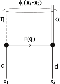
Figure 1: The schematic diagram of the $d+d\rightarrow\eta+\alpha$ reaction.

In this section, we consider the $d+d\rightarrow(\eta+\alpha)\rightarrow X$ reaction and explain our theoretical model developed in this article. In the experiments of this reaction at WASA-at-COSY Krzemien:2015fsa ; Krzemien:2014qma ; Krzemien:2014ywa ; Adlarson:2013xg ; Skurzok:2016fuv ; Skurzok:2011aa , the total energy of the system is varied by changing the deuteron beam momentum around the $\eta+\alpha$ threshold energy, which corresponds to the beam momentum $p=2.3$ GeV/$c$, and the $\eta+\alpha$ bound state production signal is expected to be observed as peak structures of the cross section of the $d+d\rightarrow{{}^{3}\rm He}+p+\pi^{-}$ and $d+d\rightarrow{{}^{3}\rm He}+n+\pi^{0}$ reactions in the energy region below the $\eta$-$\alpha$ production threshold energy region.

Based on these considerations, we have developed a phenomenological model described below. In the model, the fusion and $\eta$ meson production processes are phenomenologically parameterized and the Green’s function technique is used to sum up all $\eta$-$\alpha$ final states.

First we formulate the transition amplitude for the $d+d\to\eta+\alpha$ reaction. We adopt the framework of the hadron reaction phenomenologically. We take a model in which the $\eta$ meson production and the $d+d\to\alpha$ fusion take place in a finite size region as schematically pictured in Fig. 1. All the information on the finiteness of the reaction range, the spacial dimensions of the nuclear sizes, the structure of the deuterons and the alpha and overlap of their wavefunctions is represented by transition form factor $F(\vec{q})$. We are interested in the $\eta$ production at the threshold, so that the final state, $\eta$ and $\alpha$, is dominated by $s$ wave and, thus, the total spin-parity of the final state with a pseudo scalar ($\eta$) and a scalar ($\alpha$) bosons is $0^{-}$. Deuteron having spin 1 is represented by a axial vector boson. According to Lorenz invariance, pseudoscalar $0^{-}$ state can be made out of two axial-vectors $1^{+}$ by so-called anomalous coupling like $\epsilon^{\mu\nu\rho\sigma}\partial_{\mu}A_{\nu}\partial_{\rho}A_{\sigma}PS$, where $A_{\mu}$ and $P$ are an axial-vector boson and a pseudoscalar boson, respectively. $S$ is a scalar boson. Thus, the interaction Hamiltonian may be written as

$${\cal H}_{\rm int} = -ic\epsilon^{ijk}((\partial_{x_{2}^{0}}\nabla^{i}_{x_{1}}-\partial_{x_{1}^{0}}\nabla^{i}_{x_{2}})\hat{\phi}^{j}_{d}(x_{1})\hat{\phi}^{k}_{d}(x_{2}))\,$$ (1)

$$\hat{\phi}_{\eta}^{\dagger}(x_{1})\hat{\phi}_{\alpha}^{\dagger}(x_{2})\,{\cal F}(x_{1},x_{2})$$

where $\hat{\phi}^{i}_{d}(x)$ is the deuteron field operator with spin index $i$, $\hat{\phi}_{\eta}^{\dagger}(x)$ and $\hat{\phi}_{\alpha}^{\dagger}(x)$ are the creation operators for $\eta$ and $\alpha$, respectively, and $c$ expresses the interaction strength. The interaction strength $c$ will be adjusted so as to reproduce the observed cross section. The function ${\cal F}(x_{1},x_{2})$ in Eq. (1) represents non-local transition form factor of $d+d\to\eta+\alpha$, which is supposed to include the information on the $d+d\to\alpha$ fusion, and the $\eta$ meson production in the hadronic interaction such as $N+N\to\eta+N+N$. Assuming the translational invariant, we define the Fourier transformation

$${\cal F}(x_{1},x_{2})=\int\frac{d^{4}q}{(2\pi)^{4}}F(\vec{q})e^{iq\cdot(x_{1}-x_{2})}.$$ (2)

The momentum transfer $\vec{q}$ of the reaction is large and all nucleons should participate in the fusion reaction equally. Since it is hard to calculate $F(\vec{q})$ in a microscopic way, we treat it phenomenologically and assume a functional form of $F(\vec{q})$ in the numerical evaluation.

Letting the wave functions of the incident deuterons labeled by $d_{1}$ and $d_{2}$ be given by plane waves with momentum $p_{1}$ for deuteron $d_{1}$ and $p_{2}$ for deuteron $d_{2}$ and writing the wave functions of $\eta$ and $\alpha$ in the final state as $\phi_{\eta}^{\dagger}(\vec{x})e^{-iE_{\eta}x^{0}}$ and $\phi_{\alpha}^{\dagger}(\vec{x})e^{-iE_{\alpha}x^{0}}$ with the $\eta$ and $\alpha$ energies $E_{\eta}$ and $E_{\alpha}$, respectively, we obtain the connected part of the $S$-matrix in the center of mass frame:

$$S = -i{\cal N}_{d_{1}}{\cal N}_{d_{2}}{\cal N}_{\eta}{\cal N}_{\alpha}c\int d^{4}x_{1}d^{4}x_{2}\epsilon^{ijk}(\partial_{x_{2}^{0}}\nabla^{i}_{x_{1}}-\partial_{x_{1}^{0}}\nabla^{i}_{x_{2}})$$

$$\left[\chi_{d_{1}}^{j}\chi_{d_{2}}^{k}e^{-ip_{1}\cdot x_{1}}e^{-ip_{2}\cdot x_{2}}+\chi_{d_{2}}^{j}\chi_{d_{1}}^{k}e^{-ip_{2}\cdot x_{1}}e^{-ip_{1}\cdot x_{2}}\right]$$

$$\times\int\frac{d^{4}q}{(2\pi)^{4}}F(\vec{q})e^{iq\cdot(x_{1}-x_{2})}\phi^{*}_{\eta}(\vec{x}_{1})e^{iE_{\eta}x_{1}^{0}}\phi^{*}_{\alpha}(\vec{x}_{2})e^{iE_{\alpha}x^{0}_{2}}$$

where $\chi_{d_{1}}$ and $\chi_{d_{2}}$ are the spin wave functions for deuteron $d_{1}$ and $d_{2}$, respectively, and the normalization factors ${\cal N}_{i}$ are given as ${\cal N}_{i}=\sqrt{M_{i}/E_{i}}$ with mass $M_{i}$ and energy $E_{i}$. Operating the derivatives onto the wave functions, we have the $S$-matrix as

$$S = -i2\pi\delta(E_{1}+E_{2}-E_{f}){\cal N}_{d_{1}}{\cal N}_{d_{2}}{\cal N}_{\eta}{\cal N}_{\alpha}$$ (4)

$$\times c\int d\vec{x}_{1}d\vec{x}_{2}\epsilon^{ijk}2(E_{2}p_{1}^{i}-E_{1}p_{2}^{i})\chi_{d_{1}}^{j}\chi_{d_{2}}^{k}e^{i\vec{p}_{1}\cdot\vec{x}_{1}}e^{i\vec{p}_{2}\cdot\vec{x}_{2}}$$

$$\times\int\frac{d\vec{q}}{(2\pi)^{3}}F(\vec{q})e^{-i\vec{q}\cdot(\vec{x}_{1}-\vec{x}_{2})}\phi^{*}_{\eta}(\vec{x}_{1})\phi^{*}_{\alpha}(\vec{x}_{2}),$$

where $E_{1}$ and $E_{2}$ are the energies for deuteron $d_{1}$ and $d_{2}$, respectively, $E_{f}=E_{\eta}+E_{\alpha}$ and the integrations in terms of the time components provide energy conservation

$$\int dx_{1}^{0}dx_{2}^{0}\frac{dq_{0}}{2\pi}e^{-ix_{1}^{0}(E_{1}-q^{0}-E_{\eta})}e^{-ix_{2}^{0}(E_{2}+q^{0}-E_{\alpha})}$$

$$=2\pi\delta(E_{1}+E_{2}-E_{f}).$$ (5)

In order to perform the spacial integrals, we introduce the relative coordinate for the final state, $\vec{R}$ and $\vec{r}$, defined as

$$\vec{R} = \frac{m_{\eta}\vec{x}_{1}+M_{\alpha}\vec{x}_{2}}{m_{\eta}+M_{\alpha}},$$ (6)

$$\vec{r} = \vec{x}_{1}-\vec{x}_{2}.$$ (7)

We also introduce the wave function for the relative motion of the final state, $\phi_{f}(\vec{r})$, and assume that the center of mass motion of the $\eta$ and $\alpha$ system is written as the plane wave. This implies that we replace the $\eta$ and $\alpha$ wave functions as follows:

$${\cal N}_{\eta}{\cal N}_{\alpha}\phi_{\eta}(\vec{x}_{1})\phi_{\alpha}(\vec{x}_{2})\to{\cal N}_{f}e^{i\vec{p}_{f}\cdot\vec{R}}\phi_{f}(\vec{r}),$$ (8)

with the momentum of the center of motion $\vec{p}_{f}=\vec{p}_{\eta}+\vec{p}_{\alpha}$ and the normalization of the wave function of relative motion $\phi_{f}(\vec{x})$ given as $\int d\vec{x}|\phi_{f}(\vec{x})|^{2}=1.$ In this coordinate, the $S$-matrix is written as

$$S = -i2\pi\delta(E_{1}+E_{2}-E_{f}){\cal N}_{d_{1}}{\cal N}_{d_{2}}{\cal N}_{f}$$

$$\times c\epsilon^{ijk}2(E_{2}p_{1}^{i}-E_{1}p_{2}^{i})\chi_{d_{1}}^{j}\chi_{d_{2}}^{k}$$

$$\times\int d\vec{R}d\vec{r}\,e^{i(\vec{p}_{1}+\vec{p}_{2})\cdot\vec{R}}\,e^{i(\frac{M_{\alpha}}{m_{\eta}+M_{\alpha}}\vec{p}_{1}-\frac{m_{\eta}}{m_{\eta}+M_{\alpha}}\vec{p}_{2})\cdot\vec{r}}$$

$$\times\int\frac{d\vec{q}}{(2\pi)^{3}}F(\vec{q})e^{-i\vec{q}\cdot\vec{r}}\phi^{*}_{f}(\vec{r})e^{-i\vec{p}_{f}\cdot\vec{R}}.$$

The integral in terms of $\vec{R}$ provides momentum conservation

$$\int d\vec{R}e^{i(\vec{p}_{1}+\vec{p}_{2}-\vec{p}_{f})\cdot\vec{R}}=(2\pi)^{3}\delta(\vec{p}_{1}+\vec{p}_{2}-\vec{p}_{f}).$$ (9)

Introducing the Fourier transform

$$\phi_{f}(\vec{r})=\int\frac{d\vec{p}}{(2\pi)^{3}}\tilde{\phi}_{f}(\vec{p})e^{-i\vec{p}\cdot\vec{r}},$$ (10)

we perform the spacial integrals and obtain

$$S = -i(2\pi)^{4}\delta^{(4)}(p_{1}+p_{2}-p_{f}){\cal N}_{d_{1}}{\cal N}_{d_{2}}{\cal N}_{f}$$ (11)

$$\times c\epsilon^{ijk}2(E_{2}p_{1}^{i}-E_{1}p_{2}^{i})\chi_{d_{1}}^{j}\chi_{d_{2}}^{k}$$

$$\times\int\frac{d\vec{q}}{(2\pi)^{3}}F(\vec{q})\tilde{\phi}^{*}_{f}(\vec{P}),$$

where $\vec{P}$ is defined as $\displaystyle\vec{P}=\frac{M_{\alpha}}{m_{\eta}+M_{\alpha}}\vec{p}_{1}-\frac{m_{\eta}}{m_{\eta}+M_{\alpha}}\vec{p}_{2}-\vec{q}$.

In the center of mass frame, $E_{1}=E_{2}\equiv E_{d}$ and $\vec{p}_{1}=-\vec{p}_{2}\equiv\vec{p}$. Since the $T$ matrix is given by $S=1-iT(2\pi)^{4}\delta^{(4)}(p_{1}+p_{2}-p_{f}){\cal N}_{d_{1}}{\cal N}_{d_{2}}{\cal N}_{f}$, we obtain the $T$-matrix in the center of mass fram as

$$T=4cE_{d}\,\vec{p}\cdot(\vec{\chi}_{d_{1}}\times\vec{\chi}_{d_{2}})\tilde{F}(\vec{p}),$$ (12)

where we have defined $\tilde{F}(\vec{p})$ as

$$\tilde{F}(\vec{p})\equiv\int\frac{d\vec{q}}{(2\pi)^{3}}F(\vec{q})\tilde{\phi}^{*}_{f}\left(\vec{p}-\vec{q}\right).$$ (13)

With this $T$-matrix the cross section of the fusion with $\eta$ production can be obtained as

$$d\sigma=\frac{1}{9}\sum_{\chi_{d_{1}},\chi_{d_{2}},f}\frac{|T|^{2}}{8p_{\rm c.m.}E_{d}}(2\pi)^{4}\delta^{(4)}(p_{i}-p_{f})\frac{d\vec{p}_{f}}{(2\pi)^{3}2E_{f}},$$ (14)

where $p_{\rm c.m.}=|\vec{p}|$ and we take average for the initial spin and sum up all the possible final states. Performing the integral in terms of $\vec{p}_{f}$ and taking spin sum, we obtain

$$\sigma=\frac{2\pi}{9}c^{2}p_{\rm c.m.}\sum_{f}|\tilde{F}(\vec{p})|^{2}\delta(E_{i}-E_{f}),$$ (15)

where we have used $E_{i}=2E_{d}=E_{f}$.

The total cross section can be written with the Green’s function of the $\eta$ meson. Using Eq.(13), we have

$$\sum_{f}|\tilde{F}(\vec{p})|^{2}\delta(E_{f}-E_{i})$$ (16)

$$= \frac{1}{(2\pi)^{6}}\sum_{f}\delta(E_{f}-E_{i})\int d\vec{q}_{1}\,d\vec{r}_{1}F(\vec{q}_{1})e^{-i(\vec{q}_{1}-\vec{p})\cdot\vec{r}_{1}}\phi^{*}_{f}(\vec{r}_{1})$$

$$\times\int d\vec{q}_{2}\,d\vec{r}_{2}F^{*}(\vec{q}_{2})e^{i(\vec{q}_{2}-\vec{p})\cdot\vec{r}_{2}}\phi_{f}(\vec{r}_{2}).$$

The sum over the final states provides the inclusive spectrum and can be evaluated by using Green’s function method as follows: Using the formula $\displaystyle\delta(x)=-\frac{1}{\pi}{\rm Im}\frac{1}{x+i\epsilon}$ for an infinitesimal quantity $\epsilon$, we obtain

$$\sum_{f}\delta(E_{f}-E_{i})\phi_{f}^{*}(\vec{r}_{1})\phi_{f}(\vec{r}_{2})$$ (17)

$$= -\frac{1}{\pi}{\rm Im}\sum_{f}\phi^{*}_{f}(\vec{r}_{1})\frac{1}{E_{f}-E_{i}+i\epsilon}\phi_{f}(\vec{r}_{2})\ \ \$$

$$= -\frac{1}{\pi}{\rm Im}\sum_{f}\phi^{*}_{f}(\vec{r}_{1})\frac{1}{\hat{H}-E_{i}+i\epsilon}\phi_{f}(\vec{r}_{2}),$$ (18)

where we have used the fact that the wave function $\phi_{f}(\vec{r})$ is an eigenfunction of the Hamiltonian $\hat{H}$ for the $\eta$–$\alpha$ system. Equation (18) is an representation of Green’s operator $(\hat{H}-E_{i}+i\epsilon)^{-1}$ in terms of the eigenfunction of the Hamiltonian. Thus, we write the Green’s function in the coordinate space as $G(E_{i};\vec{r}_{1},\vec{r}_{2})$, and we have

$$\sigma = \frac{2}{9}c^{2}p_{\rm c.m.}$$

$$\times (-){\rm Im}\int d\vec{r}_{1}d\vec{r}_{2}f(\vec{r}_{1})e^{i\vec{p}\cdot r_{1}}G(E_{i};\vec{r}_{1},\vec{r}_{2})f^{*}(\vec{r}_{2})e^{-i\vec{p}\cdot\vec{r}_{2}},$$

where we have introduced the coordinate space expression of $F(\vec{q})$ as

$$f(\vec{r})\equiv\int\frac{d\vec{q}}{(2\pi)^{3}}F(\vec{q})e^{-i\vec{q}\cdot\vec{r}}.$$ (20)

Further by assuming the spherically symmetric form of $f$ for simplicity, we replace $f({\vec{r}})$ as,

$$f({\vec{r}})\rightarrow f(r).$$ (21)

And by making use of the multipole expansion of $G$,

$$G(E_{i};{\vec{r}_{1}},{\vec{r}_{2}})=\sum_{\ell m}Y_{\ell m}(\hat{r}_{1})Y_{\ell m}^{*}(\hat{r}_{2})G^{\ell}(E_{i};r_{1},r_{2}),$$ (22)

we obtain the final form of $\sigma$ as,

$$\sigma = -\frac{8\pi}{9}c^{2}p_{\rm c.m.}\ {\rm Im}\int r_{1}^{2}dr_{1}r_{2}^{2}dr_{2}\ f(r_{1})f^{*}(r_{2})$$ (23)

$$\times \sum_{\ell}(2\ell+1)\ j_{\ell}(pr_{1})\ G^{\ell}(E_{i};r_{1},r_{2})\ j_{\ell}(pr_{2}),$$

where $j_{\ell}$ is the spherical Bessel function. This expression is used for the numerical evaluation of the fusion cross section of Eq. (15).

We can divide the total cross section $\sigma$ into two parts, the conversion part $\sigma_{\rm conv}$ and the escape part $\sigma_{\rm esc}$ as,

$$\sigma=\sigma_{\rm conv}+\sigma_{\rm esc},$$ (24)

based on the identity

$${\rm Im}G=\{G^{\dagger}{\rm Im}UG\}+\{(1+G^{\dagger}U^{\dagger}){\rm Im}G_{0}(1+UG)\},$$ (25)

where $G_{0}$ is the free Green’s function of $\eta$ and $U$ the $\eta$-nucleus potential Green . The first term of the R.H.S of Eq. (25) represents the contribution of the $\eta$ meson absorption by the imaginary part of the $\eta$-nucleus potential $U$ and is called as the conversion part. The second term is the contribution from the $\eta$ meson escape from the nucleus and is called as the escape part.

The conversion part of the cross section $\sigma_{\rm conv}$ is evaluated by the practical form written as,

$$\sigma_{\rm conv} = -\frac{8\pi}{9}c^{2}p_{\rm c.m.}\int r_{1}^{2}dr_{1}r_{2}^{2}dr_{2}r_{3}^{2}dr_{3}\ f(r_{1})f^{*}(r_{3})$$ (26)

$$\times {\rm Im}U_{\rm opt}(r_{2})\sum_{\ell}(2\ell+1)j_{\ell}(pr_{1})$$

$$\times G^{\ell*}(E_{i};r_{1},r_{2})\ G^{\ell}(E_{i};r_{2},r_{3})\ j_{\ell}(pr_{3}),$$

for the spherical $\eta$-$\alpha$ optical potential $U_{\rm opt}(r)$. We calculate the escape part as $\sigma_{\rm esc}=\sigma-\sigma_{\rm conv}$.

The conversion and escape parts have the different energy dependence. In the subthreshold energy region of the $\eta$ meson production, the total cross section $\sigma$ is equal to the conversion part $\sigma_{\rm conv}$ since the energy of the $\eta$ meson is insufficient to escape from the nucleus and all $\eta$ mesons must be absorbed to the nucleus finally. Thus, the signal of the formation of the $\eta$ bound state is expected to be observed in $\sigma_{\rm conv}$. As shown in Eq. (26), the expression of the conversion cross section $\sigma_{\rm conv}$ includes the Green’s function $G^{\ell}$ which is responsible for the peak and cusp structures in the spectrum as the consequences of the $\eta$-nucleus interaction such as the bound state formation with angular momentum $\ell$. For higher partial waves $\ell$ without any bound states, the energy dependence of $G^{\ell}$ is tend to be rather mild and almost flat in the energy region of the $\eta$ production threshold. In addition, $\sigma_{\rm conv}$ also includes ${\rm Im}U_{\rm opt}$ and, thus, the size of $\sigma_{\rm conv}$ will be larger for stronger absorptive potential. Consequently, as shown later, the flat contribution to the conversion spectrum gets larger in proportional to the strength of the absorptive potential. Above the threshold of $\eta$ production, we have also the contribution from the escape processes. This escape part $\sigma_{\rm esc}$ can be compared to the observed $\eta$ production cross section in the $d+d\rightarrow\eta+\alpha$ reaction.

We should mention here to the effects of the distortion of the initial deuterons to the calculated results. In Eq. (LABEL:eq:S), the deuteron waves are introduced to the formula as plane waves. The distortion effects will modify the deuteron-deuteron relative wave function and could change the results. In the present cases, however, we can expect the effects will be minor in the final spectra shown in next section by the following reasons. The energy range of the final spectra considered in this article is very narrow and restricted to only around the $\eta$ production threshold. Thus, the distortion effects between two deuterons are almost constant in this narrow energy range and are expected to change only absolute value of the spectra by an almost constant factor. On the other hand, in the present analyses, we normalize the calculated results using the experimental data of $d+d\rightarrow\eta+\alpha$ reaction observed above the threshold as we will see later. Thus, the final results are expected to be insensitive to the deuteron distortion. We have checked qualitatively this statement by introducing the spherical distortion factor to suppress the contributions from the small relative coordinate region in Eqs. (23) and (26), and we have confirmed that the distortion effects to the spectra is almost constant within the accuracy of around 15 % in the energy region considered here. Hence, we can neglect the deuteron distortion effects in this article.

As for the numerical evaluation, we assume the $\eta$-$\alpha$ optical potential has the following form,

$$U_{\rm opt}(r)=(V_{0}+iW_{0})\frac{\rho_{\alpha}(r)}{\rho_{\alpha}(0)},$$ (27)

where $V_{0}$ and $W_{0}$ are the parameters to determine the potential strength at center of the $\alpha$ particle. The density of the $\alpha$ particle $\rho_{\alpha}(r)$ is assumed to have Gaussian form,

$$\rho_{\alpha}(r)=\rho_{\alpha}(0)\exp\left[-\frac{r^{2}}{a^{2}}\right],$$ (28)

with the range parameter $a=1.373$ fm which reproduces the R.M.S radius of $\alpha$ to be 1.681 fm. The central density of this distribution is $\rho_{\alpha}(0)=0.28~{}{\rm fm}^{-3}\simeq 1.6\rho_{0}$ with the normal nuclear density $\rho_{0}=0.17$ fm^-3. As the practical form of $F$, we assume the Gaussian as,

$$F({\vec{p}})=(2\pi)^{3/2}\left(\frac{2}{p_{0}^{2}\pi}\right)^{3/4}\exp\left[-\frac{p^{2}}{p_{0}^{2}}\right],$$ (29)

in this article and we treat $p_{0}$ as a phenomenological parameter. We also show the numerical results obtained by choosing other functional forms for the transition form factor $F({\vec{p}})$ ($f({\vec{r}})$) in Appendix to estimate the functional form dependence of our results.

We make a few comments on the difficulties for developing more microscopic model to evaluate the reaction rate. The first difficulty is the large momentum transfer. We need around 1 GeV/$c$ momentum transfer at the $\eta$ production threshold in the center of mass frame. The accuracy of the microscopic wave function in such high momentum transfer region is not well investigated. Another difficulty arises from the fact that the reaction is a fusion reaction. In the fusion reaction, all particles in the system participate the reaction equally and receive large momentum transfer. Because of these features of this reaction, we need the sufficiently accurate wave function of the five-body system (four nucleons and one $\eta$ meson) and the reliable description of the fusion and $\eta$ production processes to perform the fully microscopic calculation.

On the other hand, at the same time, we can also find an advantage for the studies of this reaction. We can make use of the experimental data of the $d+d\rightarrow\eta+\alpha$ reaction just above the $\eta$ production threshold Frascaria:1994va ; Willis:1997ix ; Wronska:2005wk . These data must provide us important information on the reaction and can be used to fix the parameters included in the present model. It should be also mentioned that the energy spectrum of the $\eta$-$\alpha$ system is expected to be simple since the system is small and may have only a few bound levels of $\eta$ even if they exist. The simple spectrum could be helpful to identify the bound levels from the data.

3 Numerical Results and Discussions

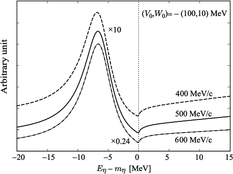
Figure 2: Calculated total cross sections of the $d+d\rightarrow(\eta+\alpha)\rightarrow X$ reaction for the formation of the $\eta$-$\alpha$ bound system with $p_{0}=400,500,600$ MeV/$c$ cases plotted as functions of the $\eta$ excited energy $E_{\eta}-m_{\eta}$. The parameters of the $\eta$-$\alpha$ optical potential are fixed to be $(V_{0},W_{0})=-(100,10)$ MeV. It is noted that the result with $p_{0}=600$ MeV/$c$ is scaled by factor $0.24$ and that with $p_{0}=400$ MeV/$c$ scaled by factor 10.

The theoretical model described in section 2 includes three parameters, which are the strength of the real and imaginary parts of the $\eta$-$\alpha$ potential ($V_{0},W_{0}$) defined in Eq. (27), and the parameter $p_{0}$ appeared in Eq.(29) to determine the property of the function $F$ which physical meanings are explained in Eqs. (1) and (2).

We study first the sensitivity of the shape of the cross section to the parameter $p_{0}$. We show the calculated total cross section $\sigma$ in Eq. (23) for $p_{0}=400,500,600$ MeV/$c$ cases with $(V_{0},W_{0})=-(100,10)$ MeV as functions of the $\eta$ excited energy $E_{\eta}-m_{\eta}$ in Fig. 2. The peak structure of the results with $p_{0}=400$ MeV/$c$ is small and is located on the top of almost flat spectrum. We find that the structures appearing in the cross section is insensitive to $p_{0}$ and almost same for three $p_{0}$ values. Thus, we fix the value of this parameter to be $p_{0}=500$ MeV/$c$ in the following numerical results and focus on the sensitivity of the structure of the spectrum to the $\eta$-$\alpha$ potential strength.

The parameter $p_{0}$ dependence of the total cross section can be understood by considering the change of spatial dimension of the $f(\vec{r})$ defined in Eq. (20). For smaller $p_{0}$ value, the distribution of $F$ in the momentum space is more compact and that of $f$ in coordinate space is wider. Thus, for smaller $p_{0}$ values, we have relatively larger contributions of higher partial wave $\ell$ of the $\eta$ meson in the calculation of the cross section in Eq. (23), which are expected not to have any structures as function of energy around the threshold as mentioned before. Hence, for smaller $p_{0}$ values, the small peak structure appears on the top of the almost flat contribution in the spectrum.

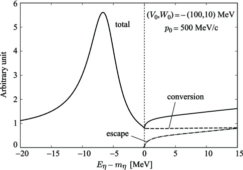
Figure 3: Calculated cross section of the $d+d\rightarrow(\eta+\alpha)\rightarrow X$ reaction for the formation of the $\eta-\alpha$ bound system plotted as functions of the $\eta$ excited energy $E_{\eta}-m_{\eta}$. The parameters of the $\eta$-$\alpha$ optical potential are $(V_{0},W_{0})=-(100,10)$ MeV, and the parameter $p_{0}$ is fixed to be $p_{0}=500$ MeV/$c$. The thick solid line indicates the total cross section $\sigma$. The dashed line and the dot-dashed line indicate the conversion part $\sigma_{\rm conv}$ and the escape part $\sigma_{\rm esc}$, respectively.

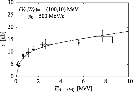
Figure 4: Calculated escape part $\sigma_{\rm esc}$ in Fig. 3 plotted with the experimental data of $d+d\rightarrow\eta+\alpha$ reaction indicated by black squares Frascaria:1994va , black circles Willis:1997ix , and open circles Wronska:2005wk . The parameters of the $\eta$-$\alpha$ optical potential are $(V_{0},W_{0})=-(100,10)$ MeV and the parameter $p_{0}$ is fixed to be $p_{0}=500$ MeV/$c$. The height of the calculated spectrum is adjusted so as to reproduce the data by changing the interaction strength $c$ given in Eq. (1).

In Fig. 3, we show again the calculated $\sigma$ for the case with parameters $(V_{0},W_{0})=-(100,10)$ MeV for $p_{0}=500$ MeV/$c$ to study the detail structure of the spectrum. Three lines correspond to the total cross section $\sigma$, the conversion part $\sigma_{\rm conv}$, and the escape part $\sigma_{\rm esc}$. The $\eta$ production threshold corresponds to $E_{\eta}-m_{\eta}=0$ and the $\eta$-$\alpha$ bound states are expected to be produced in the subthreshold region $E_{\eta}-m_{\eta}<0$. We can see in Fig. 3 that the spectrum has non-trivial structures above the flat contribution whose height seems to be about 1 in the scale of the vertical axis. There is a clear peak at $E_{\eta}-m_{\eta}\simeq-7$ MeV which corresponds to the formation of the $\eta$-$\alpha$ bound state. The calculated escape part is plotted with data in Fig. 4. We have adjusted the height of the spectrum by the interaction strength $c$ in Eq. (1). The agreement of the spectrum shapes of the calculated results and the data above the threshold seems reasonably good in this potential parameter. Hence, this observation implies that this parameter set, which predicts the formation of $\eta$-$\alpha$ bound state, does not contradicts to the $d+d\rightarrow\eta+\alpha$ data above threshold. We will make further comments for the comparison with the subthreshold data later in this section.

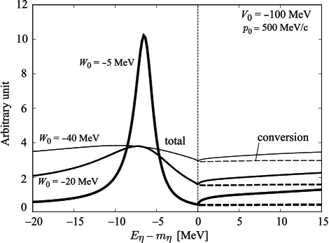
Figure 5: Calculated cross sections of the $d+d\rightarrow(\eta+\alpha)\rightarrow X$ reaction for the formation of the $\eta-\alpha$ bound system plotted as functions of the $\eta$ excited energy $E_{\eta}-m_{\eta}$. The parameters of the $\eta$-$\alpha$ optical potential are $(V_{0},W_{0})=-(100,5),-(100,20)$, and $-(100,40)$ MeV, and the parameter $p_{0}$ is fixed to be $p_{0}=500$ MeV/$c$. The solid lines indicate the total cross sections $\sigma$ and the dashed lines the conversion parts $\sigma_{\rm conv}$.

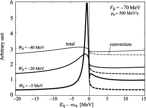
Figure 6: Same as Fig. 5 except for $(V_{0},W_{0})=-(70,5),-(70,20)$, and $-(70,40)$ MeV.

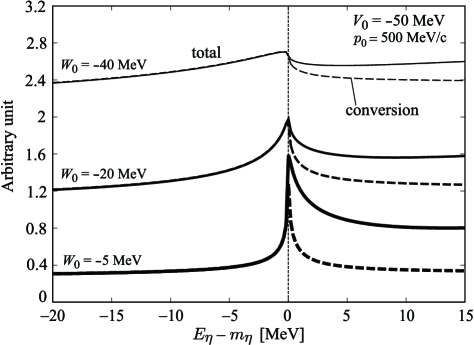
Figure 7: Same as Fig. 5 except for $(V_{0},W_{0})=-(50,5),-(50,20)$, and $-(50,40)$ MeV.

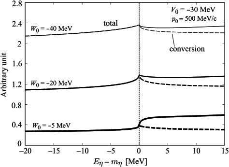
Figure 8: Same as Fig. 5 except for $(V_{0},W_{0})=-(30,5),-(30,20)$, and $-(30,40)$ MeV.

In Fig. 5, we show the results for $(V_{0},W_{0})=-(100,5)$, $-(100,20)$ and $-(100,40)$ MeV cases with $p_{0}=500$ MeV/$c$ to see the effects of the strength of the imaginary potential $W_{0}$ to the spectra. We can see from the figures the structure of the spectra below threshold $E_{\eta}-m_{\eta}<0$ is sensitive to the value of the potential parameters $W_{0}$ and is expected to be the good observables to investigate the $\eta$-nucleus interaction. Actually, the subthreshold spectrum with small imaginary potential $W_{0}=-5$ MeV clearly shows the existence of the bound state around $E_{\eta}-m_{\eta}=-7$ MeV as a peak structure. The width of the peak becomes wider and the peak height lower for larger $|W_{0}|$ value. At the same time we can see that the structure of the spectra above the threshold $E_{\eta}-m_{\eta}>0$ are relatively insensitive to the imaginary part of the $\eta$-nucleus interaction and the value of $W_{0}$.

We also show the calculated results for different $V_{0}$ and $W_{0}$ values in Figs. 6, 7 and 8. It could be interesting to note that the depth of the $\eta$-nucleus potential by the chiral unitary model in Refs. Inoue:2002xw ; GarciaRecio:2002cu is roughly close to $-(50,40)$ MeV at normal nuclear density for real and imaginary parts, respectively. The depth of the so-called $t\rho$ potential evaluated by using the $\eta$-$N$ scattering length $a_{\eta N}=(0.28+0.19i)$ fm in Ref. Bhalerao:1985cr is around $-(30,20)$ MeV at normal nuclear density. It should be noted that the parameters $V_{0}$ and $W_{0}$ adopted here in Eq. (27) indicate the potential strength at the center of the $\alpha-$particle where $\rho_{\alpha}(0)\simeq 0.28$ fm^-3 as defined in Eq. (28). The $\eta$-$\alpha$ potential also has been studied microscopically in Refs. Rakityansky:1996gw ; Kelkar:2007pn ; Fix:2017ani , where the various values of the $\eta$-$\alpha$ scattering length $a_{\eta\alpha}$ were reported. We could compare our potential strength ($V_{0},W_{0}$) with the scattering length simply by the Born approximation as $\displaystyle a_{\eta\alpha}=-2\mu\int drr^{2}U_{\rm opt}(r)$ with the $\eta$-$\alpha$ reduced mass $\mu$. For example, based on this relation, some of the potential parameters used in this article correspond to the scattering length as,

•

$(V_{0},W_{0})=-(100,5)$ MeV  $\leftrightarrow$  $a_{\eta\alpha}=2.81+0.14i$ fm

•

$(V_{0},W_{0})=-(70,20)$ MeV  $\leftrightarrow$  $a_{\eta\alpha}=1.97+0.56i$ fm

•

$(V_{0},W_{0})=-(50,40)$ MeV  $\leftrightarrow$  $a_{\eta\alpha}=1.40+1.12i$ fm.

It will be interesting to compare these numbers with the microscopic scattering lengths, for example, results of the microscopic calculation listed in Table IV in Ref. Fix:2017ani . We can see that the potential strengths adopted in this article are within the range of uncertainties of microscopic calculation.

We find again the same tendencies in these results as in Fig. 5. In Fig. 6 for $V_{0}=-70$ MeV case, we also find the bound state peak at $E_{\eta}-m_{\eta}\simeq-1$ MeV which is very clear for small $|W_{0}|$ case. In the result shown in Fig. 7 for $V_{0}=-50$ MeV case, we find the cusp structure at the threshold energy, which becomes less prominent for larger absorption potential. In Fig. 8, for weaker attractive cases with $V_{0}=-30$ MeV, we find the step like structure at the threshold for weak absorptive case with $W_{0}=-5$ MeV, which becomes less prominent again for stronger absorptive potential with larger $|W_{0}|$ value. From these figures, we find that the total spectra around and below threshold $E_{\eta}-m_{\eta}\leq 0$ are sensitive to both the real and imaginary parts of the $\eta$-nucleus interaction described by the parameters ($V_{0},W_{0}$) and are good observables to obtain information on the $\eta$-nucleus interaction.

As shown in the conversion spectra in Figs. 5–8, we have the almost flat contributions in whole energy region as mentioned in Sect. 2. This flat contribution is considered to be a part of the background cross sections of the experimental data. Thus, we subtract the flat contribution in the conversion part in the following numerical results to investigate the structure appearing in the spectrum. For this purpose, we subtract the minimum value of the conversion cross section in the energy range shown in the following figures.

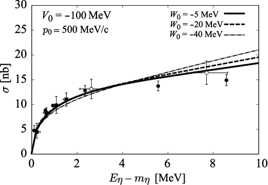
Figure 9: Calculated escape part $\sigma_{\rm esc}$ plotted with the experimental data of $d+d\rightarrow\eta+\alpha$ reaction indicated by black squares Frascaria:1994va , black circles Willis:1997ix , and open circles Wronska:2005wk . The parameters of the $\eta$-$\alpha$ optical potential are $(V_{0},W_{0})=-(100,5),-(100,20)$, and $-(100,40)$ MeV as shown in the figure. The parameter $p_{0}$ is fixed to be $p_{0}=500$ MeV/$c$.

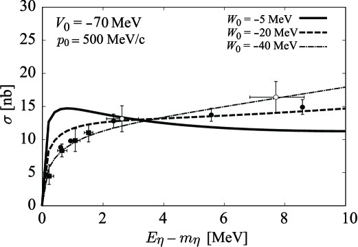
Figure 10: Same as Fig. 9 except for the $\eta$-$\alpha$ optical potential parameters are $(V_{0},W_{0})=-(70,5),-(70,20)$, and $-(70,40)$ MeV as shown in the figure.

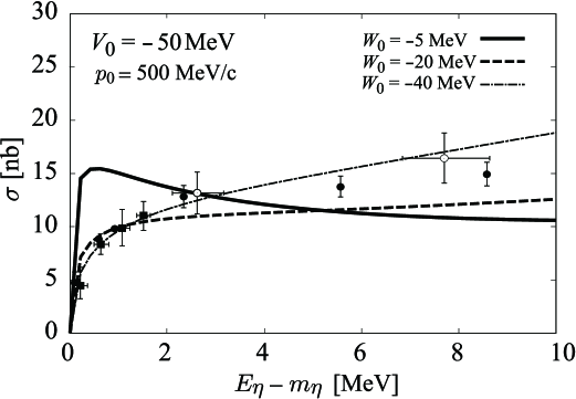
Figure 11: Same as Fig. 9 except for the $\eta$-$\alpha$ optical potential parameters are $(V_{0},W_{0})=-(50,5),-(50,20)$, and $-(50,40)$ MeV as shown in the figure.

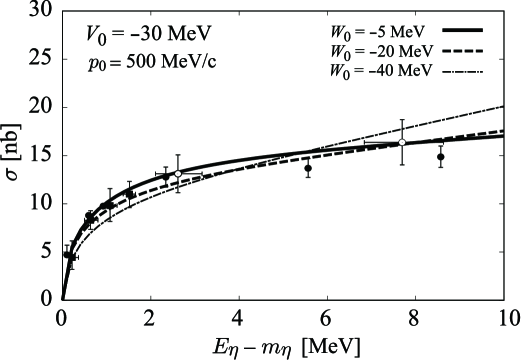
Figure 12: Same as Fig. 9 except for the $\eta$-$\alpha$ optical potential parameters are $(V_{0},W_{0})=-(30,5),-(30,20)$, and $-(30,40)$ MeV as shown in the figure.

It will be extremely interesting to show the binding energies and widths of the $\eta$-$\alpha$ bound states obtained by solving the Klein-Gordon equation using the same $\eta$-$\alpha$ potential used to calculate the spectra in Figs. 5–8. The results are compiled in Table 1. We find that only peak structures appearing in the spectra for the strong attractive–weak absorptive potential cases correspond to the existence of the bound states. Other structures in the spectra may not indicate the existence of the bound state, though they provide important information on the $\eta$-$\alpha$ interaction definitely.

Table 1: Calculated binding energies (B.E.) and widths ($\Gamma$) of the $\eta$-$\alpha$ bound states by solving the Klein-Gordon equation with the optical potential defined in Eq. (27). All states shown here are ground states. We have not found any bound states for $V_{0}=-50$ and $-30$ MeV with $W_{0}=-5,-20,-40$ MeV cases.

$W_{0}$	$V_{0}=-100$ MeV		$V_{0}=-70$ MeV
[MeV]	B.E.	${\rm\Gamma}$	B.E.	${\rm\Gamma}$
$-5$	6.4	2.7	0.5	1.1
$-20$	5.7	11.0	-	-
$-40$	3.3	22.9	-	-

Now, we focus on the escape part of the spectrum which appears above the threshold, $E_{\eta}-m_{\eta}>0$, and can be compared to the experimental data of the $d+d\rightarrow\eta+\alpha$ reaction as already shown in Fig. 4 for a certain parameter set. In Fig. 9, we show the calculated escape part of the spectra for $V_{0}=-100$ MeV cases with different strengths of the absorptive potential together with the experimental data. The calculated results are scaled to fit the experimental data by changing the interaction strength $c$. As we can see from Figs. 4 and 9, the shape of the escape part is relatively insensitive to the value of the potential parameter $W_{0}$ in this case.

We also show the calculated results of the escape part with different potential parameters in Figs. 10,  11 and  12 for different strengths of the attractive potential. We find that the shape of the escape part is not very sensitive to the $V_{0}$ and $W_{0}$ parameters and that it could be uneasy to obtain the detail information on $\eta$-nucleus potential only from the escape parts. Although we have some cases which could be safely ruled out by these comparison, such as $(V_{0},W_{0})=-(70,5)$ and $-(50,5)$ MeV cases, in which we find a distinct threshold structure as shown in Figs. 10 and 11, the whole shape of the calculated results are not so much different from that of experimental data in many cases.

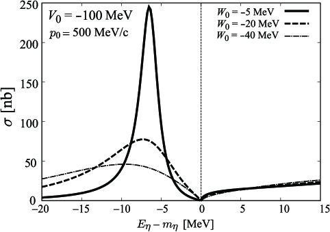
Figure 13: Calculated total cross sections of $d+d\rightarrow(\eta+\alpha)\rightarrow X$ reaction scaled by the same factor used in Fig. 9 plotted as functions of the $\eta$ excited energy $E_{\eta}-m_{\eta}$. The flat contributions are subtracted. The parameters of the $\eta$-$\alpha$ optical potential are $(V_{0},W_{0})=-(100,5),-(100,20)$, and $-(100,40)$ MeV, and the parameter $p_{0}$ is fixed to be $p_{0}=500$ MeV/$c$.

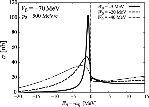
Figure 14: Calculated total cross sections of $d+d\rightarrow(\eta+\alpha)\rightarrow X$ reaction scaled by the same factor used in Fig. 10 plotted as functions of the $\eta$ excited energy $E_{\eta}-m_{\eta}$. The flat contributions are subtracted. The parameters of the $\eta$-$\alpha$ optical potential are $(V_{0},W_{0})=-(70,5),-(70,20)$, and $-(70,40)$ MeV, and the parameter $p_{0}$ is fixed to be $p_{0}=500$ MeV/$c$.

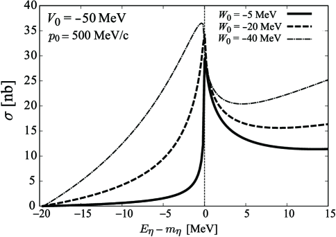
Figure 15: Calculated total cross sections of $d+d\rightarrow(\eta+\alpha)\rightarrow X$ reaction scaled by the same factor used in Fig. 11 plotted as functions of the $\eta$ excited energy $E_{\eta}-m_{\eta}$. The flat contributions are subtracted. The parameters of the $\eta$-$\alpha$ optical potential are $(V_{0},W_{0})=-(50,5),-(50,20)$, and $-(50,40)$ MeV, and the parameter $p_{0}$ is fixed to be $p_{0}=500$ MeV/$c$.

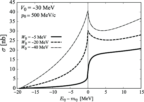
Figure 16: Calculated total cross sections of $d+d\rightarrow(\eta+\alpha)\rightarrow X$ reaction scaled by the same factor used in Fig. 12 plotted as functions of the $\eta$ excited energy $E_{\eta}-m_{\eta}$. The flat contributions are subtracted. The parameters of the $\eta$-$\alpha$ optical potential are $(V_{0},W_{0})=-(30,5),-(30,20)$, and $-(30,40)$ MeV, and the parameter $p_{0}$ is fixed to be $p_{0}=500$ MeV/$c$.

One of the best ways to obtain the decisive information on the $\eta$-nucleus interaction may be to have the direct experimental observation of the $\eta$-nucleus spectrum below the threshold, where the spectrum shape is more sensitive to the potential parameters as shown in Figs. 5–8, especially if a bound state exists. Nevertheless, it could happen that nature might not give us any bound states or our experimental techniques would not be sufficient to distinguish a less prominent peak due to a large width. In such cases, we could deduce the information on the $\eta$-nucleus interaction from the absolute value of the spectrum below the $\eta$-nucleus threshold in comparison with the $\eta$ production cross section in the same reaction above the threshold.

Here we have a model which can be used to calculate both the conversion and escape parts in the same footing simultaneously. The conversion part describes the spectrum shape induced by the $\eta$ absorption to the nucleus, while the escape part shows the $\eta$ production cross section. In our model, we leave the interaction strength of the $d+d\rightarrow\eta+\alpha$ given in Eq. (1) as a free parameter. We can adjust this parameter so as to reproduce the $\eta$ production data by the escape part of our spectrum, and then the conversion part can be a outcome from the model. Since the conversion part of the spectrum below the threshold is more sensitive to the $\eta$-nucleus interaction parameters, comparing the theoretical prediction and experimental data of the $d+d$ reaction below the threshold, we can deduce the information on the interaction parameters.

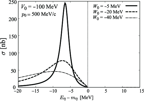
Figure 17: Calculated conversion part of cross sections of $d+d\rightarrow(\eta+\alpha)\rightarrow X$ reaction scaled by the same factor used in Fig. 9 plotted as functions of the $\eta$ excited energy $E_{\eta}-m_{\eta}$. The flat contributions are subtracted. The parameters of the $\eta$-$\alpha$ optical potential are $(V_{0},W_{0})=-(100,5),-(100,20)$, and $-(100,40)$ MeV, and the parameter $p_{0}$ is fixed to be $p_{0}=500$ MeV/$c$.

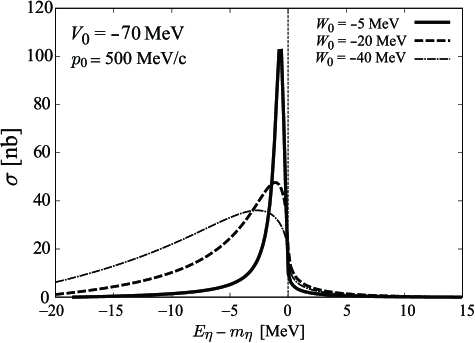
Figure 18: Calculated conversion part of cross sections of $d+d\rightarrow(\eta+\alpha)\rightarrow X$ reaction scaled by the same factor used in Fig. 10 plotted as functions of the $\eta$ excited energy $E_{\eta}-m_{\eta}$. The flat contributions are subtracted. The parameters of the $\eta$-$\alpha$ optical potential are $(V_{0},W_{0})=-(70,5),-(70,20)$, and $-(70,40)$ MeV, and the parameter $p_{0}$ is fixed to be $p_{0}=500$ MeV/$c$.

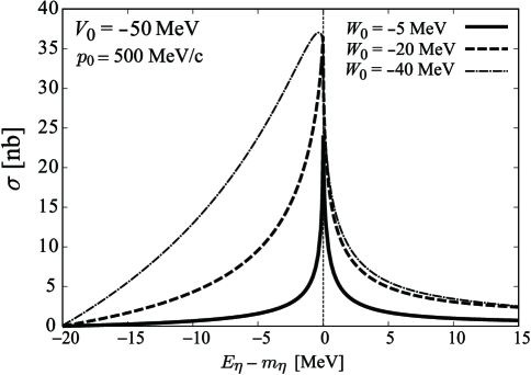
Figure 19: Calculated conversion part of cross sections of $d+d\rightarrow(\eta+\alpha)\rightarrow X$ reaction scaled by the same factor used in Fig. 11 plotted as functions of the $\eta$ excited energy $E_{\eta}-m_{\eta}$. The flat contributions are subtracted. The parameters of the $\eta$-$\alpha$ optical potential are $(V_{0},W_{0})=-(50,5),-(50,20)$, and $-(50,40)$ MeV, and the parameter $p_{0}$ is fixed to be $p_{0}=500$ MeV/$c$.

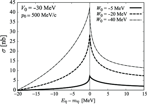
Figure 20: Calculated conversion part of cross sections of $d+d\rightarrow(\eta+\alpha)\rightarrow X$ reaction scaled by the same factor used in Fig. 12 plotted as functions of the $\eta$ excited energy $E_{\eta}-m_{\eta}$. The flat contributions are subtracted. The parameters of the $\eta$-$\alpha$ optical potential are $(V_{0},W_{0})=-(30,5),-(30,20)$, and $-(30,40)$ MeV, and the parameter $p_{0}$ is fixed to be $p_{0}=500$ MeV/$c$.

For the purpose, we show the scaled theoretical total cross section of the $d+d\rightarrow(\eta+\alpha)\rightarrow X$ reaction in Figs. 13–16 for various values of the parameter ($V_{0},W_{0}$). The absolute value of the cross section in these figures are determined so that the escape part of the cross section reproduces the experimental data of $d+d\rightarrow\eta+\alpha$ and the nonstructural flat contributions described above are subtracted in the conversion part. We should mention here that the structure of the spectra in these figures is enhanced for smaller $|W_{0}|$ values in Figs. 13 and 14, while it is suppressed for smaller $|W_{0}|$ values in Figs. 15 and 16. This behavior can be understood by considering the origin of the structure of the spectrum. For the strong attractive potential cases, since the structure is dominated by the peak due to the existence of the bound state, the peak structure becomes more prominent for the weaker imaginary because of the smaller width of the bound state. On the other hand, for the weak real potential cases, since the structure is dominated by the absorptive processes, the structure can be suppressed for the weaker absorptive potentials.

For comparison of our calculated results with experimental data for the subthreshold energies, we show only the conversion part, since in experiment the system energy is measured by observing a pion, nucleon and a residual nucleus emitted due to $\eta$ absorption and this process is counted in the conversion part in the calculation. In Figs. 17–20, we show the calculated conversion parts of the spectra which correspond to the $\eta$ absorption processes. The obtained spectra shown in Figs. 17–20 can be compared to the shape of the experimental spectra on the background reported in Ref. Adlarson:2016dme , where the upper limit of the peak structure of the $d+d\rightarrow{{}^{3}\rm He}+n+\pi^{0}$ is 3–6 nb. This implies that the experimental upper limit for the semi-inclusive conversion spectrum of $d+d\rightarrow(\eta+\alpha)\rightarrow{\rm{}^{3}He}+N+\pi$ including both $n+\pi^{0}$ and $p+\pi^{-}$ channel could be estimated to be 3–6 nb $\times 3=$ 9–18 nb because of the isospin symmetry of the decay channel of the $\eta$-$\alpha$ system. In this case, the peak structures of the bound states in Figs. 17 and 18 are fully rejected and strong attractive with less absorptive potentials are not allowed. In addition, the upper limit provides the strong restriction to the $\eta$-$\alpha$ potential and only weak potential cases with small $|V_{0}|$ and $|W_{0}|$ values such as $(V_{0},W_{0})=-(50,5)$ and $-(30,5)$ cases could be allowed by the limit.

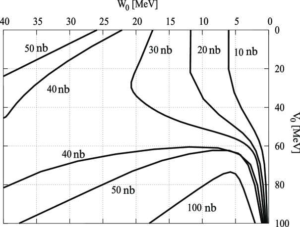
Figure 21: Contour plot of the height of the structure appearing in the conversion spectra such as shown in Figs. 17–20 in the $V_{0}-W_{0}$ plane. This plot shows clearly the acceptable region of the potential strength for various values of the upper limit of the height of the structure in the $d+d\rightarrow{{}^{3}\rm He}+N+\pi$ reaction.

In order to understand the meaning of the experimental upper limit and the results of our analyses more clearly, we plot a contour plot of the height of the structure appeared in the conversion spectra on the flat contribution in the $V_{0}-W_{0}$ plane in Fig. 21, where the acceptable region of $V_{0}$, $W_{0}$ values can be easily understood for each value of the upper limit of the height of the structure in the conversion spectra such as shown in Figs. 17–20. From this figure, the upper limit reported in Ref. Adlarson:2016dme is found to provide very valuable information on $\eta$-nucleus interaction and strongly suggests the small $|V_{0}|$ and $|W_{0}|$ values. However, it should be noted that the results in Fig. 21 are considered to be qualitative since we have not considered the experimental energy resolution here. In addition, the shapes of the structure appearing in Figs. 17–20 are not simply the symmetric peak. We also need to understand the origin of the absorptive potential and branching ratio of various decay processes to compare our results to the data for the specific decay mode. Actually, we have only considered one-nucleon absorption process for $\eta$ meson here. Multi-nucleon processes are also possible in reality Kulpa:1998vj . Thus, for deducing the quantitative information on $\eta$-nucleus interaction, it is mandatory to make the detail comparison between the calculated results and data by taking account of the realistic experimental energy resolution, asymmetric shape of the structure appeared in the conversion spectra, the branching ratio of the decay process of $\eta$ bound states and so on, especially for subthreshold energy region, where the spectra may have variety of structures depending on the $\eta$-nucleus interaction strength.

Finally, we mention the effects of the possible energy dependence of the optical potential. The optical potential has the energy dependence in general and the dependence could change the calculated spectra. To simulate the energy dependence of $\eta$-$\alpha$ optical potential, we adopted the energy dependence of the $\eta$-nucleon scattering length in Ref. Cieply:2013sya and we assumed the $\eta$-nucleon relative energy to be the quarter of that of the $\eta$-$\alpha$. The potential strength are normalized at the threshold energy. The calculated results are shown in Figs. 22 and 23. We have found that the energy dependence of the imaginary part of the optical potential mainly affects the strength of the conversion part in the spectra and changes the flat contribution of conversion part to the slope with some gradient. Hence, this effect could be important for the more realistic analyses. Though, there are many theoretical models for $\eta$-nucleon scattering length as compiled in Ref. Cieply:2013sga , the qualitative features seems common for all models.

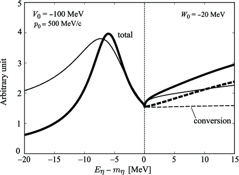
Figure 22: Calculated cross sections of the $d+d\rightarrow(\eta+\alpha)\rightarrow X$ reaction for the formation of the $\eta-\alpha$ bound system plotted as functions of the $\eta$ excited energy $E_{\eta}-m_{\eta}$. The parameters of the $\eta$-$\alpha$ optical potential is $(V_{0},W_{0})=-(100,20)$ MeV, and the parameter $p_{0}$ is fixed to be $p_{0}=500$ MeV/$c$. The solid lines indicate the total cross sections $\sigma$ and the dashed lines the conversion parts $\sigma_{\rm conv}$. The thin lines are the results with the energy independent optical potential and the thick lines are those with the energy dependent optical potential (see text).

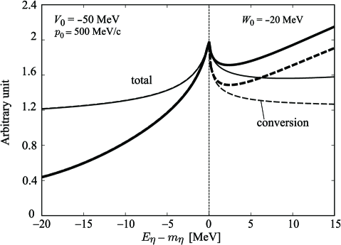
Figure 23: Same as Fig. 22 except for $(V_{0},W_{0})=-(50,20)$ MeV.

4 Conclusion

We have developed a theoretical model to evaluate the formation rate of the $\eta$-$\alpha$ bound states in the $d+d$ fusion reaction. Because of the difficulties due to the large momentum transfer which is unavoidable to produce $\eta$ meson in the fusion reaction, we formulate the model in a phenomenological way. We have shown the numerical results for the cases with the various sets of the $\eta$-nucleus interaction parameters.

We have found that the data of $\eta$ production above threshold provide important information on the absolute strength of the reaction by comparing them with the escape part of the calculated results. The upper limit of the formation cross section of the $\eta$ mesic nucleus reported in Ref. Skurzok:2016fuv also provides the significant information on the strength of the $\eta$-nucleus interaction. We would like to stress here that simultaneous fit to both data of $d+d\rightarrow\eta+\alpha$ and $d+d\rightarrow(\eta+\alpha)\rightarrow X$ using our model make it possible to provide valuable information on $\eta$-nucleus interaction. The results of our analyses are compiled in Fig. 21 as a contour plot of the $V_{0}-W_{0}$ plane.

The present discussion is simply based on the value of the upper limit of the peak structure in the fusion reaction spectrum below the threshold. As for the further works, to make the analyses performed in this article more quantitative and developed, direct comparison of the spectrum shapes between the calculated results and experiments should be necessary. For this purpose, we should take account of experimental energy resolution in the calculation and consider other possibilities of the shapes of the spectrum structure by improving the $\eta$-nucleus optical potential.

Appendix A Appendix

In this appendix, we show the numerical results for the different functional form of the transition form factor. We consider the two functions defined as

$$f_{1}({\vec{r}})=\left(\frac{m}{2\pi}\right)^{1/2}\frac{e^{-mr}}{r}$$ (A.1)

with $m=p_{0}/\sqrt{6}$, and

$$f_{2}({\vec{r}})=\left(\frac{\lambda^{3}}{\pi}\right)^{1/2}e^{-\lambda r}$$ (A.2)

with $\lambda=p_{0}$ as different forms of the transition form factor. The Gaussian form defined in Eq. (29) corresponds to

$$f({\vec{r}})=\left(\frac{p_{0}^{2}}{2\pi}\right)^{3/4}\exp\left[-\frac{p_{0}^{2}r^{2}}{4}\right],$$ (A.3)

in the coordinate space. The parameters $m$ and $\lambda$ are fixed to reproduce the same ‘root mean square radius’ $\displaystyle\left(\int|f|^{2}r^{2}d\vec{r}\right)^{1/2}$ with the Gaussian form factor.

We show the calculated results with $f_{1}(\vec{r})$ in Figs. A.1–A.4 and results with $f_{2}(\vec{r})$ in Figs. A.5–A.8, which correspond to Figs. 9, 11, 17, 19 obtained with $f(\vec{r})$ with $p_{0}=500$ MeV/$c$. These results are observables which can be compared with the appropriate experimental data. We have found that all results resemble each other and that the numerical results are robust to the choice of the functional form of the transition form factor.

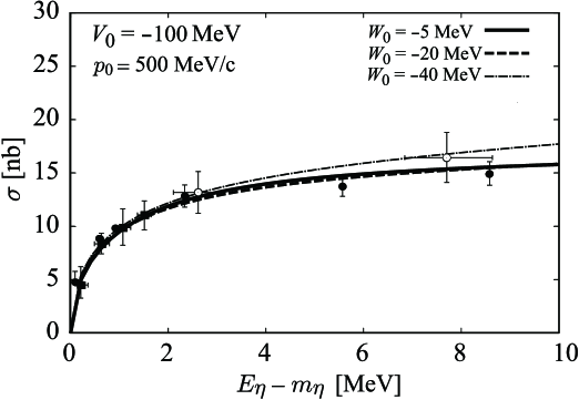
Figure A.1: Same as Fig. 9 except for the transition form factor $f_{1}(\vec{r})$ defined in Eq. (A.1) is used instead of that in Eqs. (29) and (A.3).

Figure A.2: Same as Fig. 11 except for the transition form factor $f_{1}(\vec{r})$ defined in Eq. (A.1) is used instead of that in Eqs. (29) and (A.3).

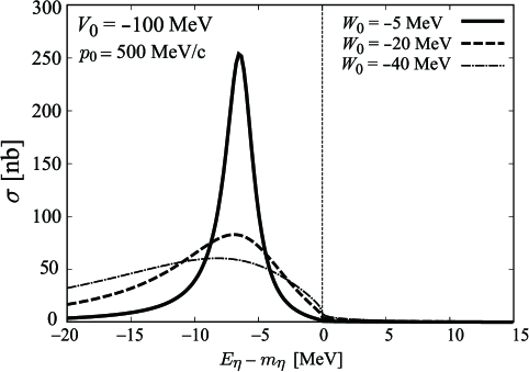
Figure A.3: Same as Fig. 17 except for the transition form factor $f_{1}(\vec{r})$ defined in Eq. (A.1) is used instead of that in Eqs. (29) and (A.3).

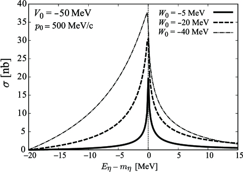
Figure A.4: Same as Fig. 19 except for the transition form factor $f_{1}(\vec{r})$ defined in Eq. (A.1) is used instead of that in Eqs. (29) and (A.3).

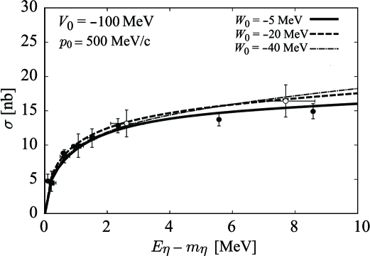
Figure A.5: Same as Fig. 9 except for the transition form factor $f_{2}(\vec{r})$ defined in Eq. (A.2) is used instead of that in Eqs. (29) and (A.3).

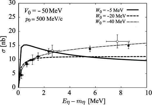
Figure A.6: Same as Fig. 11 except for the transition form factor $f_{2}(\vec{r})$ defined in Eq. (A.2) is used instead of that in Eqs. (29) and (A.3).

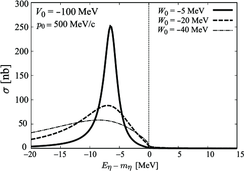
Figure A.7: Same as Fig. 17 except for the transition form factor $f_{2}(\vec{r})$ defined in Eq. (A.2) is used instead of that in Eqs. (29) and (A.3).

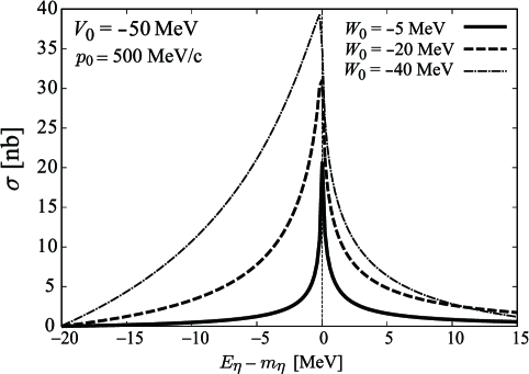
Figure A.8: Same as Fig. 19 except for the transition form factor $f_{2}(\vec{r})$ defined in Eq. (A.2) is used instead of that in Eqs. (29) and (A.3).

References

- (1) Q. Haider and L. C. Liu, Phys. Lett. B 172, (1986) 257; Phys. Rev. C 34, (1986) 1845.
- (2) R. E. Chrien et al., Phys. Rev. Lett. 60, (1988) 2595.
- (3) J. Berger et al., Phys. Rev. Lett. 61, (1988) 919.
- (4) M. Kohno and H. Tanabe, Phys. Lett. B 231, (1989) 219.
- (5) M. Kohno and H. Tanabe, Nucl. Phys. A 519, (1990) 755.
- (6) H. C. Chiang, E. Oset and L. C. Liu, Phys. Rev. C 44, (1991) 738.
- (7) G. A. Sokol and V. A. Tryasuchev, Bull. Lebedev Phys. Inst. 1991N4, 21 (1991) [Kratk. Soobshch. Fiz. 4, 23 (1991SPLRD, 4, 21–24. 1991)]; G. A. Sokol, T. A. Aibergenov, A. V. Kravtsov, A. I. L’vov, and L. N. Pavlyuchenko, Fizika B 8, 85 (1999).
- (8) J. D. Johnson et al., Phys. Rev. C 47, (1993) 2571.
- (9) T. Waas and W. Weise, Nucl. Phys. A 625, (1997) 287.
- (10) K. Tsushima, D. H. Lu, A. W. Thomas and K. Saito, Phys. Lett. B 443, (1998) 26; K. Saito, K. Tsushima, D. H. Lu and A. W. Thomas, Phys. Rev. C 59, (1999) 1203.
- (11) R. S. Hayano, S. Hirenzaki and A. Gillitzer, Eur. Phys. J. A 6, (1999) 99.
- (12) T. Inoue and E. Oset, Nucl. Phys. A 710, (2002) 354.
- (13) C. Garcia-Recio, J. Nieves, T. Inoue and E. Oset, Phys. Lett. B 550, (2002) 47.
- (14) D. Jido, H. Nagahiro and S. Hirenzaki, Phys. Rev. C 66 (2002) 045202; Nucl. Phys. A 721, (2003) 665.
- (15) H. Nagahiro, D. Jido and S. Hirenzaki, Phys. Rev. C 68, (2003) 035205.
- (16) M. Pfeiffer et al., Phys. Rev. Lett. 92, (2004) 252001.
- (17) C. Hanhart, Phys. Rev. Lett. 94, (2005) 049101.
- (18) H. Nagahiro, D. Jido and S. Hirenzaki, Nucl. Phys. A 761, (2005) 92.
- (19) N. G. Kelkar, K. P. Khemchandani and B. K. Jain, J. Phys. G 32, (2006) L19.
- (20) D. Jido, E. E. Kolomeitsev, H. Nagahiro and S. Hirenzaki, Nucl. Phys. A 811, (2008) 158.
- (21) C. Y. Song, X. H. Zhong, L. Li and P. Z. Ning, Europhys. Lett. 81, (2008) 42002.
- (22) A. Budzanowski et al. [COSY-GEM Collaboration], Phys. Rev. C 79, (2009) 012201; V. Jha et al. [GEM Collaboration], Int. J. Mod. Phys. A 22, (2007) 596.
- (23) H. Nagahiro, D. Jido and S. Hirenzaki, Phys. Rev. C 80, (2009) 025205.
- (24) Q. Haider and L. C. (L. C. )Liu, Int. J. Mod. Phys. E 24 10, (2015) 1530009.
- (25) K. P. Khemchandani, N. G. Kelkar and B. K. Jain, Nucl. Phys. A 708 (2002) 312.
- (26) K. P. Khemchandani, N. G. Kelkar and B. K. Jain, Phys. Rev. C 68 (2003) 064610.
- (27) K. P. Khemchandani, N. G. Kelkar and B. K. Jain, Phys. Rev. C 76 (2007) 069801.
- (28) J. J. Xie, W. H. Liang, E. Oset, P. Moskal, M. Skurzok and C. Wilkin, Phys. Rev. C 95 (2017) no.1, 015202.
- (29) W. Krzemien, P. Moskal and M. Skurzok, Acta Phys. Polon. B 46, (2015) 757.
- (30) W. Krzemien, P. Moskal and M. Skurzok, Few Body Syst. 55, (2014) 795.
- (31) W. Krzemien et al. [WASA-at-COSY Collaboration], Acta Phys. Polon. B 45, (2014) 689.
- (32) P. Adlarson et al. [WASA-at-COSY Collaboration], Phys. Rev. C 87, (2013) 035204.
- (33) M. Skurzok et al. [WASA-at-COSY Collaboration], Acta Phys. Polon. B 47, (2016) 503.
- (34) M. Skurzok, P. Moskal and W. Krzemien, Prog. Part. Nucl. Phys. 67, (2012) 445.
- (35) P. Adlarson et al., Nucl. Phys. A 959 (2017) 102.
- (36) N. G. Kelkar, Eur. Phys. J. A 52 (2016) no.10, 309.
- (37) R. Frascaria et al., Phys. Rev. C 50, (1994) 537.
- (38) N. Willis et al., Phys. Lett. B 406, (1997) 14.
- (39) A. Wronska et al., Eur. Phys. J. A 26, (2005) 421.
- (40) O. Morimatsu and K. Yazaki, Nucl. Phys. A 435, (1985) 727; A 483, (1988) 493.
- (41) R. S. Bhalerao and L. C. Liu, Phys. Rev. Lett. 54 (1985) 865.
- (42) S. A. Rakityansky, S. A. Sofianos, M. Braun, V. B. Belyaev and W. Sandhas, Phys. Rev. C 53 (1996) R2043. doi:10.1103/PhysRevC.53.R2043
- (43) N. G. Kelkar, Phys. Rev. Lett. 99 (2007) 210403 doi:10.1103/PhysRevLett.99.210403 [arXiv:0711.4066 [quant-ph]].
- (44) A. Fix and O. Kolesnikov, Phys. Lett. B 772 (2017) 663.
- (45) J. Kulpa and S. Wycech, Acta Phys. Polon. B 29 (1998) 3077.
- (46) A. Cieplý and J. Smejkal, Nucl. Phys. A 919 (2013) 46.
- (47) A. Cieplý, E. Friedman, A. Gal and J. Mareš, Nucl. Phys. A 925 (2014) 126.