Dipolar Bose Supersolid Stripes

Abstract

We study the superfluid properties of a system of fully polarized dipolar bosons moving in the $XY$ plane. We focus on the general case where the polarization field forms an arbitrary angle $\alpha$ with respect to the $Z$ axis, while the system is still stable. We use the diffusion Monte Carlo and the path integral ground state methods to evaluate the one-body density matrix and the superfluid fractions in the region of the phase diagram where the system forms stripes. Despite its oscillatory behavior, the presence of a finite large-distance asymptotic value in the $s$-wave component of the one-body density matrix indicates the existence of a Bose condensate. The superfluid fraction along the stripes direction is always close to 1, while in the $Y$ direction decreases to a small value that is nevertheless different from zero. These two facts confirms that the stripe phase of the dipolar Bose system is a clear candidate for an intrinsic supersolid without the presence of defects as described by the Andreev-Lifshitz mechanism.

Supersolid many-body systems appear in nature when two continuous U(1) symmetries are broken. The first one is associated to the translational invariance of the crystalline structure, while the second one corresponds to the appearance of a non-trivial global phase of the superfluid state Boninsegni_2012 . Supersolid phases were predicted to exist in Helium already in the late 60’s Andreev_69 , though their experimental observation has been ellusive. In fact, the claims for detection made at the beginning of this century have been refuted, as the observed behavior is not caused by finite non-conventional rotational inertia but rather to elastic effects Kim_2012 . In this way, a neat observation of supersolidity in ⁴He is still lacking. In fact, it is not clear yet whether a pure, defect-free supersolid structure like the one that would be expected in ⁴He really exists. Recently, the issue of supersolidity has emerged again, but now in the field of ultracold atoms. Two different experimental teams have claimed that spatial local order and superfluidity have been simultaneously observed in lattice setups Leonard_17 and in stripe phases Li_17 . In this way, the definition of what a supersolid really is seems to still be under discussion Anderson_2017 .

Superfluid properties of solid-like phases are also of fundamental interest in quantum condensed matter. One of these is the stripe phase, where the system presents spatial order in one direction but not in the others. For instance, stripe phases have been of major interest since 1990, when non-homogeneous metallic structures with broken spatial symmetry were found to favor superconductivity Bianconi_00 ; Bianconi_13 . More recently, stripe phases have been observed in Bose-Einstein condensates with synthetically created spin-orbit coupling Li_17 , where the momentum dependence of the interaction induces spatial ordering along a single direction in some regions of the phase diagram Li_13 . Stripe phases have also been discussed in the context of quantum dipolar physics, including very recent theoretical and experimental analysis of metastable striped gases of ¹⁶⁴Dy Wenzel_2017 . Due to the anisotropic character of the dipolar interaction, in some regions of the phase diagram dipoles arrange in stripes, both in Fermi Yamaguchi_10 ; Sun_10 and Bose Macia_2012 ; Macia_2014 systems. In some cases the presence of this phase has been reported to exist even in the isotropic limit Parish_12 . Though the presence of stripe phases in dipolar systems is well established and has been recently observed Kadau_2016 , it is not yet clear whether the system exhibits superfluid properties (thus forming supersolid stripes) or not.

In a previous work we determined the phase diagram Macia_2014 of the two-dimensional system of Bose dipoles at zero temperature, tracing the transition lines between the solid, gas and stripe phases. The formation and excitation spectrum of the stripe phase, where the system acquires crystal order in one direction while being fluid on the other, was previously analyzed in Ref. Macia_2012 . In this Letter we investigate the superfluid properties of the stripe phase as a function of the density and polarization angle. Our results show that dipolar stripes are a special form of supersolid, and we quantify the superfluid density and condensate fraction all along the superstripe phase.

In the following we consider a system of $N$ fully polarized dipolar bosons of mass $m$ moving on the XY plane. All dipoles are considered to be aligned along a fixed direction in space given by a polarization (electric or magnetic) field, which is contained on the XZ plane and forming and angle $\alpha$ with respect to the Z axis. The model Hamiltonian describing the system becomes then

$$H=-{\hbar^{2}\over 2m}\sum_{j=1}^{N}\nabla_{j}^{2}+{C_{dd}\over 4\pi}\sum_{i<j}^{N}\left[{1-3\lambda^{2}\cos^{2}\theta_{ij}\over r_{ij}^{3}}\right]\ ,$$ (1)

with $\lambda=\sin\alpha$, and $(r_{ij},\theta_{ij})$ the polar coordinates associated to the position vector of particle $j$ with respect to particle $i$. The constant $C_{dd}$ is proportional to the square of the (electric or magnetic) dipole moment of the components, assumed all of them to be identical. In the following we use dimensionless units obtained from the characteristic dipolar length $r_{0}=mC_{dd}/(4\pi\hbar^{2})$.

We quantify the superfluid properties of the system evaluating both the one-body density matrix and its asymptotic value (the condensate fraction), and the superfluid density. In order to do that we employ stochastic methods. We use two different quantum Monte Carlo techniques that are known to provide exact values for the energy of the system within residual statistical noise: the diffusion Monte Carlo (DMC) Hammond_94 ; Kosztin_96 and the path integral Monte Carlo (PIGS) Sarsa_2000 ; Rota_2010 methods. The DMC simulations have been performed using a second order propagator Chin_90 , while a fourth order propagator has been employed in the PIGS calculations Chin_02 . In all cases, a variational model of the ground state wave function $\Psi_{T}$ is used. In the DMC method, the guiding wave function is used for importance sampling but the ground state estimation of any observable commuting with the Hamiltonian is exact. In PIGS simulations, $\Psi_{T}$ acts as a boundary condition at the end points of the open chains representing the set of particles. It is then propagated in imaginary time to the center of the chains, where expectation values are evaluated. In this way, any contribution orthogonal to the exact ground state is wiped out. Two different models have been used in this work. In the DMC simulations, $\Psi_{T}$ has been taken to be of the Jastrow form, with a two-body correlation factor that results from the zero-energy solution of the two-body problem associated to Eq. (1) as derived in Ref. Macia_11 , matched with a long-range phononic extension as discussed in the same reference. This model must be modified when describing the stripe phase, including a one-body term $f_{1}({\bf r})$ that allows for the formation of the stripes along the $Y$ direction

$$f_{1}(\textbf{r})=\exp\left[\eta_{s}\cos\left({2\pi n_{s}y\over L_{y}}\right)\right]\ ,$$ (2)

with $L_{y}$ the box side length along the $Y$ direction, and $n_{s}$ the number of stripes in the simulation box. Notice that these two parameters are not independent, as one must guarantee the simulation box is commensurated for a fixed number of particles. In Eq. (2), $\eta_{s}$ is a variational parameter that is consistently found to be zero in the gas phase, and non-zero in the stripe phase. For the PIGS simulations, we have adopted a much simpler model based on the zero-energy solution of the isotropic ($\alpha=0$) problem, matched with a phononic tail as in Ref. Macia_2014 . Despite its simplicity, we have found no differences with the results obtained when using the same model as in the DMC case.

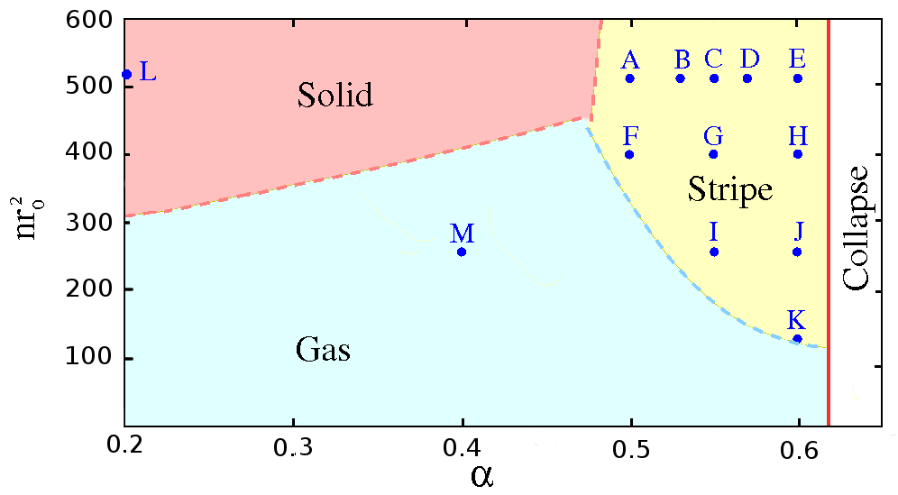
Figure 1: (color online). Phase diagram of the 2D dipolar Bose gas at zero temperature. Letters indicate the set of points corresponding to fixed density and polarization angles explored in this work.

Since we are analyzing superfluid properties, we have performed several calculations spanning a wide range of densities and polarization angles in the regions of the phase diagram where the system is in stripe form. Notice that, in the solid phase, the system arranges in a triangular lattice that completely breaks the continuous translational symmetry Macia_2014 , while in the stripe phase this symmetry is broken only in one direction (the Y axis in our setup). For the sake of comparison, we have also explored two additional points where the system remains either as a gas or as a solid. The set of points explored in this work is shown in the phase diagram, Fig. 1, and a summary of the results obtained for these points is reported in Table 1.

	$nr_{0}^{2}$	$\alpha$	$n_{0}$	$\rho_{s}$	$\rho_{s}^{x}$	$\rho_{s}^{y}$
A	512	0,50	0.00030(4)	0.86(8)	1.06(8)	0.61(8)
B	512	0.53	0.00055(6)	0.62(6)	0.99(8)	0.26(3)
C	512	0.55	0.0029(3)	0.53(5)	0.92(8)	0.14(2)
D	512	0.57	0.0031(3)	0.49(5)	0.95(8)	0.043(4)
E	512	0.60	0.0047(5)	0.49(5)	0.95(8)	0.027(3)
F	400	0.50	0.0038(3)	1.05(8)	1.07(8)	1.04(8)
G	400	0.55	0.0042(4)	0.63(6)	1.001(7)	0.26(3)
H	400	0.60	0.0052(4)	0.55(5)	1.07(8)	0.028(3)
I	256	0.55	0.015(1)	1.05(8)	1.03(8)	1.08(8)
J	256	0.60	0.011(1)	0.54(5)	1.00(8)	0.080(6)
K	128	0.60	0.071(4)	0.95(7)	0.97(7)	0.93(7)
L	512	0.20	0	0	0	0
M	256	0.40	0.019(2)	1	1	1

Table 1: Superfluid densities and condensate fraction for the points shown in Fig. 1. Figures in parenthesis are the errorbars.

A direct measure of the off-diagonal long-range order present in the system is provided by the one-body density matrix (OBDM)

$$n_{1}({\bf r}_{11^{\prime}})\!\! = \!\!\Omega\int d{\bf r}_{2}\cdots d{\bf r}_{N}$$

$$\Psi_{0}({\bf r}_{1},{\bf r}_{2},\ldots,{\bf r}_{N})\Psi_{0}({\bf r}^{\prime}_{1},{\bf r}_{2},\ldots,{\bf r}_{N})\ ,$$

with $\Psi_{0}$ the ground state wave function and $\Omega$ the volume of the container. In this way, $n_{1}({\bf r})$ is normalized such that $n_{1}(0)=1$, while $n_{1}(|{\bf r}_{11^{\prime}}|\to\infty)\to n_{0}$ if there is off-diagonal long-range order, with $n_{0}$ the condensate fraction. Notice that, in 2D, $n_{0}$ can be non-zero only at $T=0$.

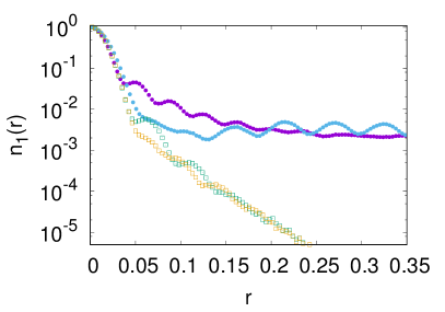
Figure 2: (color online). One Body Density Matrix of the 2D dipolar Bose system at the density $nr_{0}^{2}=512$ in the stripe phase for $\alpha=0.55$ (filled circles), and in the solid phase for $\alpha=0.20$ (empty squares). Purple circles and green squares: cuts along the X direction; blue circles and orange squares: cuts along the Y direction. Distance $r$ is measured in units of r₀. Errorbars are smaller than $10\%$ of each measure and have not been included for the sake of clarity.

Figure 2 shows a comparison of the one-body density matrix of the system at points C and L of Fig. 1, corresponding to the same density $nr_{0}^{2}=512$ but different polarization angles. In all cases $n_{1}({\bf r})$ depends on the direction due to the anisotropy of the interaction. The lower curves show two cuts of $n_{1}({\bf r})$ along the $X$ and $Y$ directions, when the system is in the solid phase (point L), while the upper curves show the same quantities for the system in the stripe phase (point C). As it can be seen, all curves show an oscillatory behavior that is partially a consequence of the anisotropy of the interaction Macia_11 . Most remarkably, the curves corresponding to the solid phase decay exponentially to zero, while the ones for the stripe phase saturate to a common value that corresponds to $n_{0}$. The condensate fraction, which appears only in the $s$-wave term of the partial wave expansion of $n_{1}({\bf r})$, has been obtained by fitting a constant to the intermediate-distance tail in regions near (but not at) half the box side where the results are stable. All values in the third column of Table 1 have been obtained in this way.

At large densities, where increasing the polarization angle makes the system change from the solid to the stripe phase, the condensate fraction increases with increasing $\alpha$. This is not surprising since the dipolar interaction is overall less repulsive when approaching the line of collapse, at the critical angle $\alpha_{c}\approx 0.615$. The situation is reversed at lower densities, when the system changes from the gas to the stripe form (point I and J for instance). In this case and close to the transition line, the condensate fraction is expected to approach higher values, as the gas is less interacting. Perpendicular cuts at fixed polarization angle and increasing density leads always to a reduction in $n_{0}$, consistent with the fact that particles have less effective space. In any case the largest values of $n_{0}$ are achieved near the gas-stripe transition line at the lowest possible densities. In this way, the large-distance limit of the OBDM of the stripe phase is always non-zero, as happens with other supersolid systems.

Even though the presence of non-zero condensate fraction value already points towards a superfluid behavior, it is possible to evaluate directly the superfluid response of the system in DMC. At finite temperature, the superfluid fraction $\rho_{s}$ is estimated from the winding number Pollock_87 , which takes into accounts the diffusion of world lines at large imaginary times. At $T=0$, this is equivalent Zhang_95 to measuing the diffusion of the center of mass of the system in the infinite imaginary time limit, according to the expression

$$\rho_{s}=\lim_{\tau\to\infty}{1\over 4N\tau}\left({D_{s}(\tau)\over D_{0}}\right)\ ,$$ (4)

where $D_{s}(\tau)=\left\langle({\bf R}_{CM}(\tau)-{\bf R}_{CM}(0))^{2}\right\rangle$ and $D_{0}=\hbar^{2}/(2m)$. For the 2D system analyzed, we identify the $X$ and $Y$ components of this expression with the superfluid fractions along the $X$ and $Y$ directions, according to $\rho_{s}=(\rho_{s}^{x}+\rho_{s}^{y})/2$.

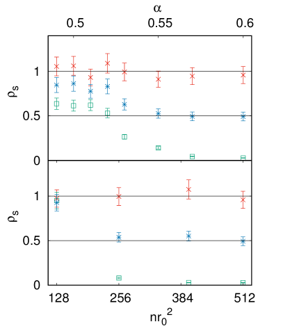
Figure 3: (color online). Superfluid fractions along the $X$ direction $\rho_{s}^{x}$ (red crosses), along the $Y$ direction $\rho_{s}^{y}$ (green squares) and total $\rho_{s}$ (blue stars). The upper panel shows the dependence of these quantities on the polarization angle at the fixed density $nr_{0}^{2}=512$. The lower panel corresponds to $\alpha=0.6$ and different densities. In all cases the system remains in the stripe phase.

Figure 3 shows our results for $\rho_{s}^{x}$, $\rho_{s}^{y}$ and the total $\rho_{s}$ for two perpendicular cuts on the phase diagram. The upper panel corresponds to a fixed density $nr_{0}^{2}=512$ and different angles in the region where the system remains in the stripe phase. The lower panel corresponds to a fixed angle $\alpha=0.6$ but different densities, also in the stripe phase. The cut at $nr_{0}^{2}=512$ and increasing $\alpha$ shows that the $X$ component of the superfluid fraction is always close to $1$, while the $Y$ component decreases to 0, leading to the overall value $\rho_{s}\approx 1/2$ near $\alpha=\alpha_{c}$. Remarkably, the total superfluid fraction $\rho_{s}$ is larger close to the transition line to the solid phase, decreasing as $\alpha$ increases. In this way, the superfluid response is discontinuous across the solid-stripe transition. The fact that $\rho_{s}^{y}$ (and thus $\rho_{s}$) decrease when $\alpha$ increases is once again a consequence of the anisotropic character of the dipolar interaction, which becomes less repulsive along the $X$ direction with increasing $\alpha$. Close to $\alpha_{c}$ the interaction along the $X$ direction is weak and particles can easily flow in each stripe, but the confinement of the stripes is stronger and the system becomes more localized along the $Y$ direction. This is confirmed by the fact that the optimal values of $\eta_{s}$ in Eq. (2) is larger when $\alpha$ approaches $\alpha_{c}$ at fixed density. A similar situation is found when the density is increased at constant $\alpha$. The lower panel of Fig. 3 show the different components of the superfluid fraction at $\alpha=0.6$ and increasing density. Once again we observe that $\rho_{s}^{y}$ decays to values close to zero already at $nr_{0}^{2}=256$, thus confirming that at high densities the confinement of the different stripes is very strong. Only point K in that line presents a large $\rho_{s}^{y}$ value, but that point is essentially in the gas-stripe transition line, and we know the total superfluid fraction $\rho_{s}=1$ in the gas phase. Contrarily to what happens when moving from the stripe to the solid phase, in the gas-stripe transition the change in $\rho_{s}$, $\rho_{s}^{x}$ and $\rho_{s}^{y}$ appears to be continuous.

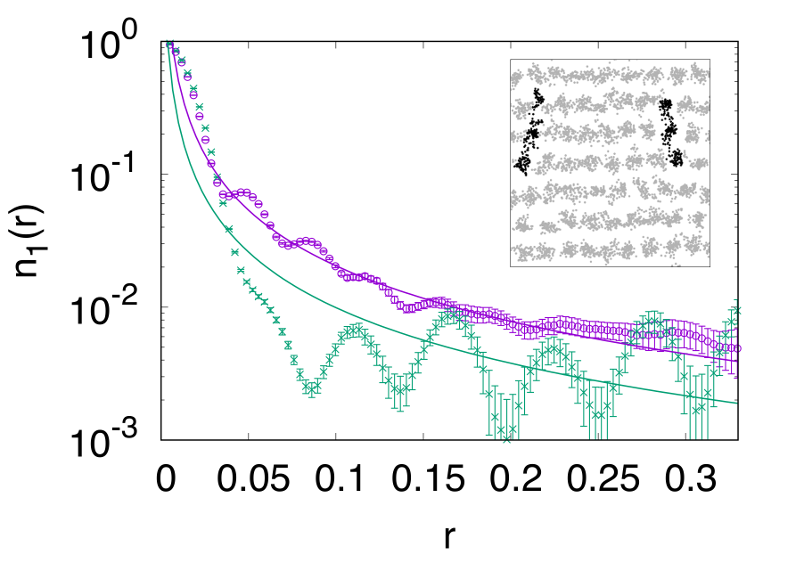
Figure 4: (color online). One-body density matrix along the $X$ (blue open squares) and $Y$ (green stars) at $\alpha=0.6$ and $nr_{0}^{2}=512$. The solid lines are fits of the form $Ax^{-1/\eta}$ with for fixed $\eta$ obtained from the slope of the static structure factor near the origin. The inset shows a snapshot of the PIGS simulation, where some of the particle exchanges are highlighted in black.

At this point, and according to the previous results, one could wonder whether stripes are so tightly confined that no particle exchanges between different stripes is possible. If that was the case, one could also think that each stripe may behave as an isolated, (quasi) 1D system. In fact and according to the results in the last column of Table 1, in some regions the $Y$ component of the superfluid fraction acquires very low values. However, it never vanishes. This indicates that, in fact, particle exchange between different stripes is always possible, though it becomes unlikely in the limits commented above.

Taking that into account, one can look for traces of a (quasi) 1D behavior in the regions where $\rho_{a}^{y}\sim 0$. One way to do that is to analyze the system as a Luttinger liquid, and to check for consistency in the values of the corresponding Luttinger parameters. In order to do that we have extracted the sound velocity $c$ from a fit of the form $|k|/2c$ to the low-$k$ behavior of the static structure factor $S({\bf k})$ evaluated both in DMC and PIGS. Once with it, we have performed a fit of the form $n_{1}(u)=Au^{-1/\eta}$ with $\eta=2\pi n/c$  Luttinger_81 to the $X$ and $Y$ components of $n_{1}({\bf r})$, with the results shown in Fig, 4. As it can be seen, the fit reproduces better the tail of $n_{1}({\bf r})$ along the $X$ direction, while strong oscillations in the $Y$ component are clearly visible and $n_{1}({\bf r})$ for ${\bf r}=(0,y)$ differs significantly from the fit. It must be kept in mind, though, that the large distance behavior of $n_{1}({\bf r})$ in Luttinger liquid theory is a decaying power law not compatible with a finite condensate fraction value, while we have seen before that the stripe phase OBDM presents a large-distance asymptotic value $n_{0}\neq 0$. In this way, the curve fits well the calculated $X$-component of the OBDM at intermediate distances only. The inset in Fig. 4 shows a snapshot of the system after thermalization in PIGS, for the same conditions $nr_{0}^{2}=512$ and $\alpha=0.6$, where a pair of examples where particle exchange between different stripes is visible, have been highlighted. It is worth recalling that since simulations in PIGS are done with open chains (with variational wave functions at the end points), it is hardly possible to see long exchange lines crossing the whole simulation box.

In summary, we have performed DMC and PIGS simulations to analyze the supersolid properties of dipolar Bose stripes in two dimensions for polarization angles before collapse. We have evaluated the one-body density matrix to find that it always presents a finite (though in some regions, quite small) condensate fraction value, in contrast to the continuously decaying tail it presents in the solid phase. We have also evaluated the superfluid fraction along the $X$ and $Y$ directions to find that, at large densities and/or polarization angles, the $Y$-component becomes very small, though it never vanishes. At high densities and polarization angles the stripes are tightly confined and the intermediate distance behavior of the OBDM along the stripe direction has a dependence on the distance that is somehow compatible with a Luttinger liquid model. However, particle exchanges, always visible in configuration snapshots, lead to a finite condensate fraction value and an overall superfluid behavior that, together with the existence of Bragg peaks Macia_2014 , confirm the supersolid character of that phase.

This work has been supported by the Ministerio de Economia, Industria y Competitividad (MINECO, Spain) under grant No. FIS2014-56257-C2-1-P.

References

- (1) M. Boninsegni, and N. V. Prokof’ev, Rev. Mod. Phys. 84, 759 (2012).
- (2) A. F. Andreev, and I. M. Lifshitz, JETP 29, 1107 (1969).
- (3) E. Kim, and M. H. W. Chan, Nature 427, 225 (2004).
- (4) D. Y. Kim, and M. H. W. Chan, Phys. Rev. Lett. 109, 155301 (2012).
- (5) J. Léonard, A. Morales, P. Zupancic, T. Esslinger, and T. Donner, Nature 543, 87 (2017).
- (6) J. R. Li, J. Lee, W. Huang, S. Burchesky, B. Shteynas, F.Ç. Top, A. O. Jamison, and W. Ketterle, Nature 543, 91 (2017).
- (7) P. W. Anderson, Physics World 30, 21 (2017).
- (8) A. Bianconi, Int. J. Mod. Phys. B, 14, 3289 (2000).
- (9) A. Bianconi, D. Innocenti, and G. Campi, Journal of Superconductivity and Novel Magnetism, 26, 2585 (2013).
- (10) Y. Li, G. I. Martone, L. P. Pitaevskii, and S. Stringari, Phys. Rev. Lett. 110, 235302 (2013).
- (11) M. Wenzel, F. Böttcher, T. Langen, I. Ferrier-Barbut, and T. Pfau, arXiv:1706.09388.
- (12) Y. Yamaguchi, T. Sogo, T. Ito, and T. Miyakawa, Phys. Rev. A 82, 013643 (2010).
- (13) K. Sun, C. Wu, and S. Das Sarma, Phys. Rev. B 82, 075105 (2010).
- (14) A. Macia, D. Hufnagl, F. Mazzanti, J. Boronat, and R. E. Zillich, Phys. Rev. Lett. 109, 235307 (2012)
- (15) A. Macia, J. Boronat, and F. Mazzanti, Phys. Rev. A 90, 061601(R) (2014).
- (16) M. M. Parish, and F. M. Marchetti, Phys. Rev. Lett. 108, 145304 (2012).
- (17) H. Kadau, M. Schmitt, M. Wenzel, C. Wink, T. Maier, I. Ferrier-Barbut, T. Pfau, Nature 530, 194-197 (2016).
- (18) B. L. Hammond, W. A. Lester Jr., and P. J. Reynolds, Monte Carlo Methods in Ab InitioQuantum Chemistry, (World Scientific, Singapore, 1994).
- (19) I. Kosztin, B. Faber, and K. Schulten, Am. J. Phys. 64(5), 633 (1996).
- (20) S. A. Chin, Phys. Rev. A 42, 6991 (1990).
- (21) A. Sarsa, K. E. Schmidt, and W. R. Magro, J. Chem. Phys. 113, 1366 (2000).
- (22) R. Rota, J. Casulleras, F. Mazzanti, and J. Boronat, Phys. Rev. E 81, 016707 (2010).
- (23) S. A. Chin, and C. R. Chen, J. Chem. Phys. 117, 1409 (2002).
- (24) A. Macia, F. Mazzanti, J. Boronat, and R. E. Zillich, Phys. Rev. A 84, 033625 (2011).
- (25) E. L. Pollock and D. M. Ceperley, Phys. Rev. B 36, 8343 (1987).
- (26) S. Zhang, N. Kawashima, J. Carlson, and J. E. Gubernatis, Phys. Rev. Lett. 74, 1500 (1995).
- (27) F. D. M. Haldane, Phys. Rev. Lett. 47, 1840 (1981).