Persistent Sinai type diffusion in Gaussian random potentials with decaying spatial correlations

Abstract

Logarithmic or Sinai type subdiffusion is usually associated with random force disorder and non-stationary potential fluctuations whose root mean squared amplitude grows with distance. We show here that extremely persistent, macroscopic ultraslow logarithmic diffusion also universally emerges at sufficiently low temperatures in stationary Gaussian random potentials with spatially decaying correlations, known to exist in a broad range of physical systems. Combining results from extensive simulations with a scaling approach we elucidate the physical mechanism of this unusual subdiffusion. In particular, we explain why with growing temperature and/or time a first crossover occurs to standard, power-law subdiffusion, with a time-dependent power law exponent, and then a second crossover occurs to normal diffusion with a disorder-renormalized diffusion coefficient. Interestingly, the initial, nominally ultraslow diffusion turns out to be much faster than the universal de Gennes-Bässler-Zwanzig limit of the renormalized normal diffusion, which physically cannot be attained at sufficiently low temperatures and/or for strong disorder. The ultraslow diffusion is also non-ergodic and displays a local bias phenomenon. Our simple scaling theory not only explains our numerical findings, but qualitatively has also a predictive character.

I Introduction

Systems with Gaussian energy disorder characterized by spatially decaying correlations are ubiquitous in physics thanks to the central limit theorem Bouchaud and Georges (1990); Bouchaud et al. (1990). Such systems include, for instance, disordered organic photoconductors with long-range electrostatic interactions Bässler (1993); Dunlap et al. (1996), supercooled liquids Bässler (1987), as well as naturally occurring DNA macromolecules encoding biological information in living systems Gerland et al. (2002); Lässig (2007); Slutsky et al. (2004). Colloidal systems in quenched, random laser-created potentials have also recently become experimentally available Evers et al. (2013); Hanes and Egelhaaf (2012); Hanes et al. (2013); Bewerunge and Egelhaaf (2016).

A common line of thinking Hänggi et al. (1990) treats diffusion and transport phenomena in such systems as normal on experimentally relevant scales, with a potential disorder-renormalized diffusion coefficient $D_{\rm ren}=D_{0}\exp(-[\beta\sigma]^{2})$, where $D_{0}$ is the free diffusion coefficient of the diffusing particle in absence of the potential, $\sigma=\langle\delta U^{2}(x)\rangle^{1/2}$ is the root-mean-squared amplitude of the potential fluctuations $\delta U(x)$, and $\beta=1/(k_{B}T)$ is the Boltzmann factor proportional to inverse temperature. This famed renormalization result by De Gennes Gennes (1975), Bässler Bässler (1987), and Zwanzig Zwanzig (1988) corresponds to a common measurable temperature dependence of transport coefficients in disordered glassy systems which is almost indistinguishable from the Vogel-Fulcher-Tammann law Hecksher et al. (2008), another commonly used temperature dependence used to fit experimental data.

It came as a surprise when extensive simulations of stochastic Langevin dynamics in Gaussian random potentials with decaying spatial correlations by Romero and Sancho Romero and Sancho (1998) demonstrated that the emerging diffusion is anomalously slow over the whole time range of simulations and characterized by a power law scaling $\langle\delta x^{2}(t)\rangle\propto t^{\alpha}$ ($0<\alpha<1$) of the mean squared displacement. This result is very remarkable indeed because within the mean field approximation it is easy to show that the Gaussian energy disorder yields residence time distributions $\psi(\tau)$ of a log-normal type in finite spatial trapping domains, all moments of which are finite. This behavior is fundamentally different from the situation of annealed exponential energetic disorder yielding residence time distributions of the form $\psi(\tau)\propto 1/\tau^{1+\alpha}$ with $\alpha=k_{B}T/\sigma$ Hughes (1995): Here subdiffusion emerges for $k_{B}T<\sigma$ because of the divergent mean residence times, which provides the standard model of subdiffusion in the continuous time random walk framework Hughes (1995); Metzler and Klafter (2000).

Hence, Gaussian energy disorder cannot yield subdiffusion in the absence of spatial correlations. To neglect such correlations is a usual procedure when they are short ranged Hänggi et al. (1990). Whether organic photoconductors and other disordered materials are better described by Gaussian or exponential models of the energy disorder is a subject of continuing controversy. On one hand, the Gaussian model is generally accepted for organic photoconductors Bässler (1993). On the other hand, some recent experiments Schubert et al. (2013) seem to be more consistent with the model of exponential disorder, leading to a similar time dependence of transient currents as in amorphous semiconductor films Scher and Montroll (1975). Models of Gaussian disorder with significant spatial correlations can be a key to resolve this controversy. Physically, for instance, such short range correlations may correspond to the size of a protein molecule diffusing over the potential landscape of a DNA strand Goychuk and Kharchenko (2014), or to the size of a colloidal particle in an uncorrelated laser field potential Hanes and Egelhaaf (2012). Morever, long-range electrostatic interactions give rise to long-range spatial correlations in organic photoconductors Dunlap et al. (1996), and biological information encoded in the sequence of DNA base pairs manifests itself in long-range base pair correlations Peng et al. (1992); ben Avraham and Havlin (2000).

The remarkable discovery that subdiffusion persists beyond the mean field approximation was reaffirmed in a number of recent studies Khoury et al. (2011); Simon et al. (2013); Hanes et al. (2013); Goychuk and Kharchenko (2014). It was explained recently in terms of a finite non-ergodicity length $L_{\rm erg}$ of the spatial random process $\exp[\beta\delta U(x)]$ Goychuk and Kharchenko (2014) related to the presence of spatial potential correlations. In this respect, the origin of a weak ergodicity breaking—the fundamental difference between ensemble and time averaged physical observables even in the limit of long observations times Bouchaud (1992); Bel and Barkai (2005); Metzler et al. (2014)—is very different from the one in systems described by continuous time random walks with annealed, uncorrelated residence time distributions with divergent mean residence times Bouchaud (1992); Bel and Barkai (2005); Burov and Barkai (2007); Lubelski et al. (2008); He et al. (2008); Sokolov et al. (2009). For systems with Gaussian disorder, the non-ergodic behavior occurs on the transient spatial scale $L_{\rm erg}$ which, however, rapidly grows with $\beta\sigma$ for spatially correlated potential fluctuations $\delta U(x)$. Indeed, this spatial scale can readily reach macroscopic sizes already for disorder strengths $\sigma\sim 4\div 5k_{B}T$, which is a typical value for disordered organic photoconductors already at room temperatures Dunlap et al. (1996).

Subdiffusion occurs on the corresponding non-ergodic and generally mesoscopic spatial scales. Somewhat surprisingly, diffusion retains its asymptotically normal form for any decaying correlations, no matter how slow they decay Goychuk and Kharchenko (2014). However, for mesoscopic and even macroscopic systems this limit can be out of reach and become physically completely irrelevant, leading us to consider this type of subdiffusion as one of the fundamental processes in a large range of applications. Some of these remarkable features have recently been confirmed experimentally in colloidal systems Hanes et al. (2013) and, more tentatively, also for diffusion of regulatory proteins on DNA strands Wang et al. (2006). Namely, although in Ref. Wang et al. (2006) the results are interpreted in terms of normal diffusion, the single-trajectory diffusion coefficient is scattered over three orders of magnitude, which likely implies a lack of ergodicity. The real physical mechanism of anomalous diffusion in spatially correlated Gaussian energetic disorder remains elusive, and it is the main goal of this paper to clarify its physical origin. The whole setup is very different from the original scenario of Sinai diffusion Sinai (1982); Bouchaud and Georges (1990); Bouchaud et al. (1990); Le Doussal et al. (1999). It is also different from Sinai diffusion emerging from a power law energy disorder ben Avraham and Havlin (2000), or logarithmic tails of the waiting time distribution Godec et al. (2014) in the mean field approximation. Notwithstanding, we will show below that a generalized Sinai subdiffusion indeed emerges at sufficiently low temperatures with $\langle\delta x^{2}(t)\rangle\propto[\ln(t/t_{0})]^{a}$, with a general scaling exponent $a$, which is $a=4$ in the special case of Sinai diffusion Sinai (1982); Bouchaud and Georges (1990); Bouchaud et al. (1990); Le Doussal et al. (1999). The latter one is usually associated with the model of random force disorder Bouchaud and Georges (1990); Bouchaud et al. (1990); ben Avraham and Havlin (2000); Le Doussal et al. (1999) yielding potential fluctuations whose root mean square amplitude exhibits an unlimited growth with distance, that is, the potential presents a free Brownian motion in space Bouchaud and Georges (1990); Bouchaud et al. (1990); Le Doussal et al. (1999). A generalized Sinai diffusion with $a\neq 4$ emerges also in the case of fractional Brownian motion in space Oshanin et al. (2013).

In this work, we reveal that a generalized Sinai type diffusion universally emerges for a sufficiently low temperature and/or strong disorder when $\beta\sigma$ exceeds a typical value of 5 to 10, even for the case of very short range exponential or linearly decaying correlations. This fundamental result is fully confirmed by extensive simulations. Based on the arguments developed herein it it should be absolutely possible to observe macroscopic Sinai diffusion at experimentally relevant time scales, in systems governed by spatially correlated Gaussian energetic disorder.

The remainder of this manuscript is structured as follows. In Section II we develop the general concepts of our approach and introduce a scaling theory for the resulting diffusive dynamics. Section III presents results from extensive simulations for various relevant cases of the spatial correlations decay of the potential fluctuations. In Section IV we present a detailed discussion of our results and draw our conclusions.

II Basic concepts and scaling theory

II.1 Growing potential fluctuations

We start from an observation, which is central to the theory of extreme events Castillo et al. (2004) and pivotal for the present study. Namely, even if a stationary Gaussian process $U(x)$ has a finite root mean squared fluctuation $\sigma$, the maximal amplitude of its fluctuations $\delta U_{\rm max}(x)$ grows slowly with the distance $x$, at odds with intuition Pickands (1969); Zhang (1986). The law of this growth can be found from the following consideration. We consider the potential as a random process with zero average, $\langle U(x)\rangle=0$, and ask the question of how often an energy level $U_{\rm max}$ is crossed with growing distance $x\to\infty$, in a stationary limit. For any stationary, differentiable Gaussian process with normalized autocorrelation function $g(x)=\langle U(x+x^{\prime})U(x^{\prime})\rangle/\sigma^{2}$ and asymptotically decaying correlations, the answer is known: The averaged number of level-crossing events $\langle n(x)\rangle$ grows linearly with distance: $\langle n(x)\rangle=\Gamma x$, at the rate $\Gamma=\sqrt{-g^{\prime\prime}(0)}\exp(-U_{\rm max}/2\sigma^{2})/\pi$ Papoulis (1991). Thus, the level $U_{\rm max}$ is typically crossed at the distance $x$ found from $\langle n(x)\rangle=1$. Hence,

$$U_{\rm max}(x)=\sigma[2\ln(x/x_{0})]^{1/2},$$ (1)

where $x_{0}=\pi/\sqrt{-g^{\prime\prime}(0)}$. This is a very general and universal result valid for any correlations with finite $g^{\prime\prime}(0)$, in agreement with the results of Ref. Pickands (1969). Note that this result holds only asymptotically, given a stationary regime is established. Moreover, the longer the correlations range, the later this asymptotic result is established.

For example, for a Gaussian decay of the correlations we will have $g(x)=\exp(-x^{2}/\lambda^{2})$ with a correlation length scale parameter $\lambda$, and in this case $x_{0}=\pi\lambda/\sqrt{2}$. Note that in a scaling sense such a correlation length parameter $\lambda$ always exists, even if the correlation length formally defined as $\lambda_{\rm corr}=\int_{0}^{\infty}|g(x)|dx$ may diverge. The length $\lambda$ plays a fundamental role in the presence of correlations. It can be, for instance, of the size of the protein-DNA contact, or the size of the colloidal particle in an uncorrelated laser field.

For power law decaying correlations with $g(x)=1/[1+x^{2}/\lambda^{2}]^{\gamma/2}$, and $g(x)\propto 1/x^{\gamma}$ for $x\gg\lambda$, and thus $x_{0}=\pi\lambda/\sqrt{\gamma}$. This case is very interesting in applications to diffusion of regulatory proteins on DNA strands, where the real base pair sequence arrangement can play a very profound role Bénichou et al. (2009); Bauer et al. (2015). In particular, longe-range correlations in the base pair sequence, which encode biological information, can indeed decay algebraically slow, as shown, for instance, in Refs. Peng et al. (1992); ben Avraham and Havlin (2000) with $\gamma\sim 0.6\div 0.8$. This should yield corresponding correlations in the protein binding energy with $\lambda$ being of the size of the protein-DNA contact, or larger. Namely, we here have a case for which $\lambda_{\rm corr}=\infty$, which suggests that the subdiffusive regime should hold much longer than in the case of short ranged correlations. This is indeed confirmed in our detailed analysis below. Another important example is provided by some organic photoconductors, for which $\gamma=1$ and $\sigma=0.1\div 0.125\;eV$ or $4\div 5\;k_{B}T$ at room temperature Dunlap et al. (1996).

The next case of relevance we consider here is the Ornstein-Uhlenbeck process with $g(x)=\exp(-|x|/\lambda)$. This case may at first appear problematic as it is not differentiable, and the corresponding force $f(x)=-\partial V(x)/\partial x$ has the infinite root mean squared amplitude $\langle f^{2}(x)\rangle^{1/2}=\infty$. However, in physical applications we consider in fact a regularized Ornstein-Uhlenbeck process on a lattice with a finite grid size $\Delta x$. This allows also for a numerical treatment of the corresponding continuous dynamics (which otherwise would not be possible due to the infinite force root mean squared amplitude). We note that this point is similar to the subtleties arising when we consider the model of white Gaussian processes $f(x)$ in the theory of continuous space Sinai diffusion Bouchaud and Georges (1990). Indeed, we always generate realizations of Gaussian processes with some finite resolution $\Delta x$, following a well established algorithm Simon et al. (2012). The corresponding $g(x)$ is getting, in fact, thereby regularized. An appropriate formal regularization reads $g(x)=\exp(-\sqrt{x^{2}+(\Delta x/2)^{2}}/\lambda+\Delta x/(2\lambda))$. It yields the same force root mean squared $\langle f^{2}(0)\rangle^{1/2}=\sqrt{2}\sigma/\sqrt{\Delta x\lambda}$ as the Ornstein-Uhlenbeck process on a lattice with grid size $\Delta x$. In this case, $x_{0}=\pi(\lambda\Delta x/2)^{1/2}$. An important further remark is that, when $\Delta x\to 0$, then $x_{0}\to 0$, and $U_{\rm max}(x)$ grows accordingly for any fixed $x$. However, this growth is logarithmically slow, and for realistic variations of $\Delta x$ the effect is small. Nevertheless, the case of exponentially decaying correlations is especially interesting in the present context. Notice that such short range correlations appear also in the case of a biologically meaningless and completely random DNA because of a finite size $\lambda$ of the protein-DNA contact, which is typically from 5 to 30 bp Stewart et al. (2012).

Another pertinent correlation model for the particular application of diffusion on DNA is the model of linearly decaying correlations $g(x)=(1-|x|/\lambda)$ for $|x|\leq\lambda$, and zero otherwise Yaglom (1972). It emerges when the protein interacts locally with only one corresponding bp, in the immediate contact. The corresponding random process $U(x)$ is also non-differentiable, and with respect to the $U_{\rm max}(x)$ behavior its regularized version behaves rather similar to that of the Ornstein-Uhlenbeck process (considered with the same $\Delta x$).

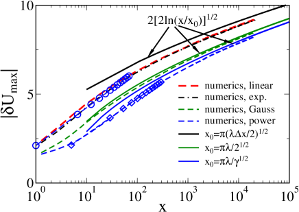
Figure 1: Maximal amplitude of potential fluctuations $|\delta U_{\rm max}(x)|$ (in units of root mean squared fluctuations $\sigma$) starting from some random point regarded as the origin, plotted versus distance $x$ (in units of the correlation length $\lambda$) for several models of Gaussian potentials with decaying correlations. This decay is (i) exponential, (ii) linear, (iii) Gaussian, and (iv) of power law form with $\gamma=0.8$. Broken lines represent the results from simulations and full lines depict the corresponding theoretical results $2U_{\rm max}(x)$ from Eq. (1), which are gradually approached for long distances $x$. In all cases, $\Delta x=0.02$ is chosen. The symbols show a $\log x$ scaling fit for either initial or intermediate values of $x$ in the case of exponential and power law models of the correlations, respectively.

Let us check the above exact analytical results against the results from extensive simulations: Fig. 1 shows how the amplitude of the potential fluctuations grows with distance for several models of Gaussian disorder. The universal result in Eq. (1) agrees well with the numerics for all four models considered here. A similar scaling was also found numerically for a different model of correlations Hanes and Egelhaaf (2012). The agreement is better for differentiable (in the limit $\Delta x\to 0$) processes, and the model of linearly decaying correlations behaves indeed rather similar to the Ornstein-Uhlenbeck model. Notice that in the case of power law decaying correlations with $\gamma=0.8$, the convergency is slower than for the Gaussian decay, and for much smaller $\gamma$, for instance, $\gamma=0.2$, it is is still far from being achieved for the largest $x$ in Fig. 1 (not shown). The results in Fig. 1 are obtained from a well-known spectral method Simon et al. (2012) given the corresponding correlation functions, on a lattice with grid size $\Delta x$ ($\Delta x=0.02$ in Fig. 1) and a maximal spatial interval $L_{\rm max}$ ($L_{\rm max}=N\Delta x,N=2^{20}$ in Fig. 1). Notice also that the exact behavior of the function $g(x)$ is used to generate the realizations of the Ornstein-Uhlenbeck process and the process with linearly decaying correlations. The shown results are obtained from averaging over $10^{3}$ uniformly distributed points (particles) in each potential realization, and $10^{2}$ such potential realizations for each model of correlations were taken.

It is clear that the strongest potential fluctuations occur in the case of exponential and linear correlations. They are further increasing for smaller values of the resolution $\Delta x$ due to the singularity of these models. Another salient feature is that another scaling can be observed transiently. Namely, we initially find the behavior $\log x$ rather than the $\sqrt{\log x}$ scaling for the exponential and linear correlations, and intermediately for the case of power law decaying correlations. Moreover, we notice an initial $(\log x)^{\delta}$ scaling with $\delta>1$ for the power law and Gaussian decay. To account for these various behaviors we henceforth consider the following model

$$|\delta U_{\rm max}(x)|=\sigma_{\rm eff}[\ln(x/x_{\rm in})]^{\delta}$$ (2)

for the potential fluctuations, where $\sigma_{\rm eff}$, $\delta$, and $x_{\rm in}$ are fitting parameters, which are generally different from the theoretical values $\sigma_{\rm eff}=2\sqrt{2}\sigma\approx 2.83\;\sigma$, $\delta=1/2$, and $x_{\rm in}=x_{0}$ in Fig. 1. We will now use this generic empirical formula and pursue the scaling argumentation used originally in the case of continuous space Sinai diffusion Bouchaud and Georges (1990).

II.2 Scaling theory

Let us estimate the time $t$ a particle needs to travel the distance $x$ starting at $x_{0}$, limited in an Arrhenius manner by the largest barrier met on its way, $t=t_{0}\exp[\beta|\delta U_{\rm max}(x)|]$, where $t_{0}$ is a proportionality factor of physical unit of time. From this scaling ansatz, in combination with relation (2) we immediately obtain our central result for the mean squared displacement of the diffusing particle,

$$\langle\delta x^{2}(t)\rangle=x_{\rm in}^{2}\left\{e^{[(k_{B}T/\sigma_{\rm eff})\ln(t/t_{0})]^{1/\delta}}-1\right\}^{2}.$$ (3)

This in turn yields the asymptotic form

$$\langle\delta x^{2}(t)\rangle\approx x_{\rm in}^{2}\left[(k_{B}T/\sigma_{\rm eff})\ln(t/t_{0})\right]^{2/\delta}$$ (4)

for small temperatures and/or strong disorder, $k_{B}T/\sigma_{\rm eff}\ll 1$. For $\delta=1/2$, this is precisely the Sinai type diffusion with $a=2/\delta=4$. However, for $\delta=1$, $\langle\delta x^{2}(t)\rangle\approx x_{\rm in}^{2}[(k_{B}T/\sigma_{\rm eff})\ln(t/t_{0})]^{2}$.

Next, with increasing temperature and time, when the unity becomes negligible in Eq. (3), we find the intermediate behavior

$$\langle\delta x^{2}(t)\rangle\approx x_{\rm in}^{2}[t/t_{0}]^{\alpha(t)}$$ (5)

with the time dependent scaling exponent

$$\alpha(t)=2(k_{B}T/\sigma_{\rm eff})^{1/\delta}\ln^{1/\delta-1}(t/t_{0}).$$ (6)

This result predicts a power-law subdiffusion with a gradually changing anomalous diffusion exponent. It should be mentioned here that this result follows from the approximation $\exp[f(t)]-1\approx\exp[f(t)]$, for a logarithmically growing $f(t)$, which is not fully accurate in our numerics. Nevertheless, it predicts the correct law for $\alpha(t)$, namely, $\alpha(t)\propto\log t$, for $\delta=1/2$, see below. This result is especially insightful for $\delta=1$ (or $\log x$ scaling): here $\alpha(t)=2k_{B}T/\sigma_{\rm eff}=\alpha_{\rm min}$, and we observe subdiffusion of power law form with a constant anomalous diffusion exponent. Moreover, given the results depicted in Fig. 1, where initially $\delta>1$, intermediately $\delta=1$, and asymptotically $\delta=1/2$, one can predict that initially $\alpha(t)$ will diminish and reach a minimum, and then logarithmically increase in time. This is what we actually see in the simulations with $\sigma_{\rm eff}\approx(1.24\div 1.52)\sigma$ within the temperature range $\sigma/4<k_{B}T<\sigma/2$, see below. Such a behavior may indeed mistakingly be attributed to continuous time random walk subdiffusion.

II.3 Transient lack of ergodicity

Due to the decaying correlations of the Gaussian potential fluctuations in our model, with increasing temperature for a given root mean squared amplitude $\sigma$ (decreasing $\beta\sigma$) and for times longer than a certain crossover time, a transition to normal diffusion will gradually emerge. The corresponding characteristic anomalous diffusion length $L_{\rm erg}$ can be found from the condition that the variance of the random process $w(x)=\exp(-\beta U(x))$ equals the mean, which yields the following implicit equation for this, so far unknown, characteristic length $L_{\rm erg}$ Goychuk and Kharchenko (2014),

$$\int_{0}^{1}\left(1-y\right)e^{\beta^{2}\sigma^{2}g(Ly)}dy=1.$$ (7)

The transition to normal diffusion starts at $\langle\delta x(t)^{2}\rangle\gtrapprox L_{\rm erg}^{2}$. However, this transition may last extremely long, and anomalous diffusion features may persist for appreciably long times for $|\delta x|>L_{\rm erg}$.

For the case of linearly decaying correlations, Eq. (7) can be solved exactly, and we obtain ($L_{\rm erg}>\lambda$)

$$L_{\rm erg} = \frac{\lambda}{(\beta\sigma)^{2}}\Big{\{}(e^{\beta^{2}\sigma^{2}}-1)-(\beta\sigma)^{2}+\Big{(}2(\beta\sigma)^{4}+4(\beta\sigma)^{2}$$ (8)

$$- 2(\beta\sigma)^{2}e^{(\beta\sigma)^{2}}+3-4e^{(\beta\sigma)^{2}}+e^{2(\beta\sigma)^{2}}\Big{)}^{1/2}\Big{\}}$$

which for $\beta\sigma\gtrapprox 2.5$ is approximated by the simple expression

$$L_{\rm erg}\approx\frac{2\lambda}{(\beta\sigma)^{2}}e^{(\beta\sigma)^{2}}$$ (9)

with a very good accuracy. For other models of $g(x)$, Eq. (7) is solved numerically, the results being listed in Table 1 for several values of $\beta\sigma$. One can see that the shortest length $L_{\rm erg}$ occurs for the linearly decaying correlations and the longest one for the power law correlations. Somewhat surprisingly, for the Gaussian decay the non-ergodicity length is larger than for exponentially decaying correlations.

$g(x)$	$\beta\sigma=2$	$\beta\sigma=3$	$\beta\sigma=4$	$\beta\sigma=5$	$\beta\sigma=10$
$e^{-|x|}$	$34.85$	$2070$	$1.2\times 10^{6}$
$e^{-x^{2}}$	$51.89$	$5027$
$\frac{1}{(1+x^{2})^{\gamma/2}}$ $\gamma=0.8$	$166.83$	$9670$	$6.86\times 10^{6}$	$4.28\times 10^{10}$	$7.64\times 10^{42}$
$1-|x|$	$24.59$	$1798$	$1.11\times 10^{6}$	$5.76\times 10^{9}$	$5.37\times 10^{41}$
$e^{\beta^{2}\sigma^{2}}$	$54.59$	$8103$	$8.89\times 10^{6}$	$7.20\times 10^{10}$	$2.69\times 10^{43}$

Table 1: Non-ergodicity length $L_{\rm erg}$ from Eq. (7), in units of $\lambda$ and values for $e^{\beta^{2}\sigma^{2}}$.

As mentioned above, there exist several crossover times in the dynamics. The first one corresponds to the transition from Sinai like diffusion to the power law diffusion regime. The corresponding transition time $\tau^{*}$ can be roughly estimated from the condition that the argument of the exponential function in Eq. (3) reaches unity. From this, $\tau^{*}\sim t_{0}\exp[\sigma_{\rm eff}/k_{B}T]$. It grows exponentially fast with $\sigma_{\rm eff}/k_{B}T$. The second transition time $\tau_{\rm erg}$ can be estimated from the condition of how long the power law diffusion regime with anomalous diffusion exponent $\alpha_{\rm min}\approx 2k_{B}T/\sigma_{\rm eff}$ will last. Thus we find the conditions $\langle x^{2}(t)\rangle\sim x_{\rm in}^{2}(\tau_{\rm erg}/t_{0})^{\alpha_{\rm min}}\sim L_{\rm erg}^{2}$, from which with $\alpha_{\rm min}\approx 2k_{B}T/\sigma_{\rm eff}$ and Eq. (9), we obtain the estimate

$$\tau_{\rm erg}\sim t_{0}\left(\frac{4\lambda^{2}}{x_{\rm in}^{2}}\frac{(k_{B}T)^{4}}{\sigma^{4}}\right)^{\frac{\sigma_{\rm eff}}{2k_{B}T}}\exp\left[\frac{\sigma^{2}\sigma_{\rm eff}}{(k_{B}T)^{3}}\right].$$ (10)

Notice the super-exponential growth of $\tau_{\rm erg}$ with $\sigma/(k_{B}T)$. This is precisely the reason why the power law subdiffusion regime can last so long already for moderate values $\sigma/(k_{B}T)\sim 4\div 5$, and no transition to the regime of normal diffusion was revealed in the concrete cases studied in Refs. Romero and Sancho (1998); Khoury et al. (2011); Simon et al. (2013).

III Results of numerical simulations

We now proceed by checking our theoretical predictions against results of extensive numerical simulations, finding remarkable agreement. To this end, let us consider a continuous-space Brownian dynamics governed by the overdamped Langevin equation

$$\eta\frac{dx(t)}{dt}=-\frac{dU(x)}{dx}+\sqrt{2k_{B}T\eta}\times\zeta(t),$$ (11)

where $\eta$ is the frictional coefficient and $\zeta(t)$ is unbiased, white Gaussian noise with $\delta$-correlation $\langle\zeta(t)\zeta(t^{\prime})\rangle=\delta(t-t^{\prime})$. Distance is scaled in units of $\lambda$, time in units of $\tau_{0}=\lambda^{2}\eta/\sigma$, and temperature in $\sigma/k_{B}$. Initially, $10^{4}$ particles are uniformly distributed in random potentials (10 realizations), and the particle motion is integrated using periodic boundary conditions with a very large period $L_{\rm max}$. The random potential is generated on a lattice with spacing $\Delta x=0.02$, and discrete points are connected by parabolic splines, that is, the potential is locally parabolic, and the corresponding force entering the Langevin equation (11) is piece-wise linear. In this respect our setup is similar to the one considered in Refs. Romero and Sancho (1998); Simon et al. (2013); Goychuk and Kharchenko (2014), but different from that in Refs. Hanes and Egelhaaf (2012); Hanes et al. (2013), where a discrete hopping dynamics in both space and time was studied. In most simulations, we employ $L_{\rm max}=2^{19}\Delta x\approx 1.0485\times 10^{4}\lambda$. We use the stochastic Heun method with a time integration step $\Delta t=2\times 10^{-4}$ in most simulations.

III.1 Exponential correlations

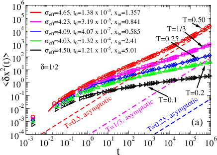
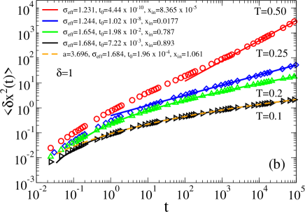
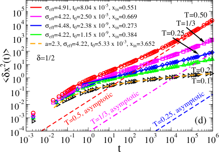
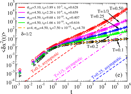
Figure 2: (Color online) Ensemble-averaged mean squared displacement (symbols) for different values of $k_{B}T$ in units of the disorder strength $\sigma$, for the four different models of spatial correlation decay: (a) and (b) exponential decay; (c) power-law decay with $\gamma=0.8$; (d) linear decay; (e) Gaussian decay. The fit of the numerical results (full lines) is performed expression (3) with $\delta=1/2$ in (a), (d), and (e); and $\delta=1$ in (b) and (c). The dashed orange line in (b) to (d) shows an alternative fit with the generalized Sinai diffusion expression (4) and $a\approx 3.70$ in (b), $a\approx 2.99$ in (c), $a\approx 2.3$ in (d), and $a\approx 4$ in (e). For $T=0.1$, Sinai diffusion covers typically at least six decades of time. Even for $T=0.5$ the fit with Eq. (3) and $\delta=1/2$ turns out to be very good over 6 decades of time, as seen in panels (a), (d), and (c). For $\delta=1/2$, $\sigma_{\rm eff}$ is typically in the range, $\sigma_{\rm eff}\sim 4\div 5.1$, whereas for $\delta=1$ it typically ranges in $\sigma_{\rm eff}\sim 1.2\div 1.7$. Distances are measured in units of $\lambda$ and time in units of $\tau_{0}=\lambda^{2}\eta/\sigma$.

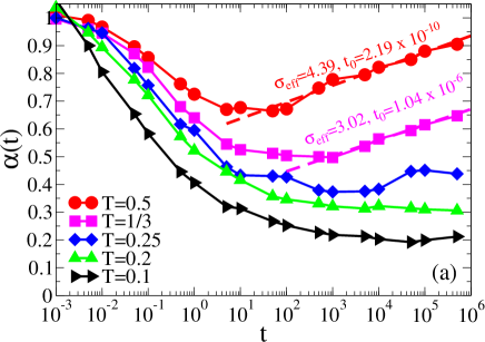
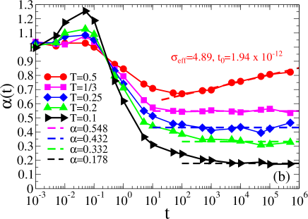
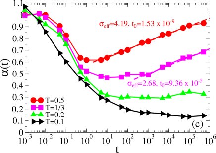
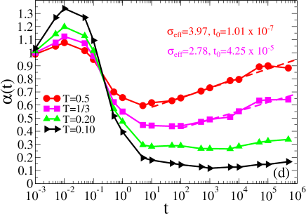
Figure 3: (Color online) Time-dependent power law exponent $\alpha_{\rm eff}(t)$ for an assumed subdiffusive law $\langle\delta x^{2}(t)\rangle\simeq t^{\alpha(t)}$ obtained as the logarithmic derivative of the traces in Fig. 2, for different temperatures in the case of (a) exponential correlations, (b) power law correlations with $\gamma=0.8$, (c) linearly decaying correlations, and (d) Gaussian correlation decay. Symbols connected by lines correspond to numerical results, while the dashed lines are fits to the dependence $\alpha(t)=2(k_{B}T/\sigma_{\rm eff})^{2}\ln(t/t_{0})$. Fitting parameters shown in the plot.

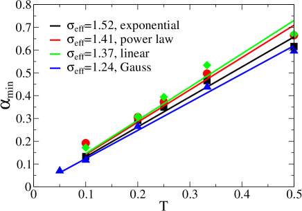
Figure 4: (Color online) Dependence of $\alpha_{\rm min}$ on temperature $T$ for the four different models of spatial correlations discussed in this paper, and the corresponding best linear fits with the dependence $\alpha\approx 2k_{B}T/\sigma_{\rm eff}$. The values of the corresponding $\sigma_{\rm eff}$ are shown in the plot.

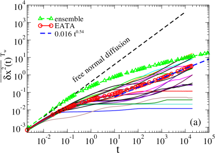
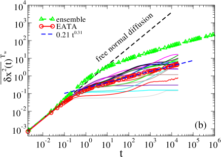
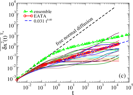
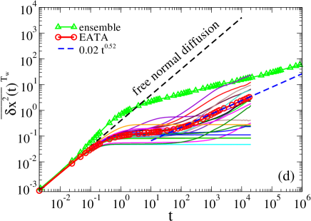
Figure 5: (Color online) Single-trajectory, time averaged mean squared displacement for $T=0.2$ and (a) exponential correlations, (b) power-law correlations with $\gamma=0.8$, (c) linearly decaying correlations, and (d) Gaussian correlation decay. The time averaging window (measurement time) was $T_{\rm w}=2\times 10^{6}$. 20 trajectory averages are depicted in each case starting from different locations. The results of the ensemble-averaged, as well as ensemble-averaged time-averaged (EATA), and free normal mean squared displacements are also depicted for comparison. The EATA mean squared displacement is nicely fitted by a power-law dependence, which is also shown in the plot. The asymptotic limit of the disorder-renormalized normal diffusion cannot be plotted for comparison because $D_{\rm ren}=\exp(-25)D_{0}\approx 1.39\times 10^{-11}D_{0}$, with $D_{0}=0.2$. Subdiffusion is by many orders of magnitude faster.

We start our numerical analysis with the case of the exponentially decaying correlations, $g(x)=\exp(-|x|)$. From the simulated trajectories, we first perform an ensemble averaging to obtain the mean squared displacement. The results are depicted in Fig. 2 in panels (a) and (b). In Fig. 2a, the fit of the numerical results is based on Eq. (3) using $\delta=1/2$, $\sigma_{\rm eff}\sim 4\div 4.7$, and $x_{\rm in}\sim 0.59\div 5.01$. Note that the fitting values $\sigma_{\rm eff}$ differ only by a factor of less than two from the theoretical value $2.83$ in Fig. 1. The corresponding theoretical value $x_{0}$ is $x_{0}\approx 0.31$. Here, the agreement is worse, however, the numerical results in Fig. 1 in this case are also somewhat different from the theoretical asymptotics, which is still not reached. The same numerical data are fitted to expression (3) with $\delta=1$ in Fig. 2b, with $\sigma_{\rm eff}\sim 1.23\div 1.69$. For $T=0.1$ and $T=0.2$, both fits have almost the same quality, although the fit with $\delta=1$ appears slightly better. For $T=0.1$, Sinai like diffusion (4) with $a\approx 3.7$, near to the Sinai value $a=4$, covers about six decades in time, Fig. 2b. It is worthwhile noting that for $T\leq 0.25$ the fit with $\delta=1$ works better, see Fig. 2b, due to the initial $\log x$ scaling in Fig. 1 (see symbols therein). For this reason, $\alpha(t)$ shows a nearly constant behavior, at intermediate temperatures, for an extended time period, Fig. 3a. In fact, in this regime the power law exponent is nearly proportional to temperature, $\alpha\approx 2k_{B}T/\sigma_{\rm eff}$, where the value of $\sigma_{\rm eff}$ is obtained from fitting the minimal value $\alpha_{\rm min}$ in Fig. 3a by this dependence. It turns out that $\sigma_{\rm eff}\approx 1.52$, Fig. 4. However, with increasing temperature, when diffusion covers larger distances, the fit with $\delta=1/2$ becomes much better, compare the case $T=0.5$ in Figs. 2a and 2b. An excellent fit holds over about six to seven decades in time with $\delta=1/2$, where the explicit time dependence of the anomalous diffusion exponent $\alpha(t)$ in Eq. (5) becomes apparent for sufficiently long times. At larger temperatures, for instance, $T=1$, the crossover to the asymptotic regime of normal diffusion is already accomplished up to $t_{\rm max}=10^{6}$ in our simulations. Such high temperatures, or weak disorder strengths, are not of interest for anomalous diffusion of the kind discussed. Generally $\alpha_{\rm eff}$ reaches a minimum $\alpha_{\rm min}$, may stay nearly constant for a certain time period, and then logarithmically increases, a dependence which can be fitted by Eq. (6) with $\delta=1/2$ and some values of $\sigma_{\rm eff}$ and $t_{0}$, which are different from those used in Fig. 2a, see Fig. 3a for $T=0.5$ and $T=1/3$. The reason for this discrepancy in the corresponding fitting values is that a transition from Eq. (3) to Eqs. (5) and (6) is still not quite justified numerically. Nevertheless, the prediction of a logarithmically increasing $\alpha(t)$, as confirmed by the simulations, is a remarkable success of our simple scaling theory.

Interestingly, our simulations demonstrate that generally the observed subdiffusion is much faster than the corresponding limit of disorder-renormalized normal diffusion, which is also shown in Fig. 2a for several values of the temperature. The presence of correlations thus leads to a dramatic increase in the particle mobility on intermediate but relevant time scales. Note that whereas for $T=0.5$ this limit is already gradually approached in Fig. 1, the corresponding asymptotics cannot even be depicted for $T=0.2$ and $T=0.1$ in this figure, as they lie outside of the plotting range, and, therefore, are completely irrelevant on the corresponding time scale.

As discussed above, the physical origin of the observed subdiffusion is due to a weak breaking of ergodicity. Hence, single trajectory time averages

$$\overline{\delta x^{2}(t)}^{\rm T_{w}}=\frac{1}{{\rm T_{w}}-t}\int_{0}^{{\rm T_{w}}-t}\Big{[}\delta x(t|t^{\prime})\Big{]}^{2}dt^{\prime}$$ (12)

of the mean-squared displacement $\delta x(t|t^{\prime})=x(t+t^{\prime})-x(t^{\prime})$ over the time window ${\rm T_{w}}$ are expected to be very different from the above ensemble result, and their amplitudes should be broadly scattered He et al. (2008); Metzler et al. (2014). This is indeed so, as evidence in Fig. 5a, where at all times $t\ll{\rm T_{w}}$, and hence this scatter is not a trivial statistical effect occurring when $t\sim{\rm T_{w}}$. Remarkably, some of the particle trajectories are quickly localized, while others are diffusing very fast. The slow ones start near to and become trapped in a low potential valley, while the fast particles start from a relatively high value of $U(x)$ and move downhill to a much lower value of $U(x)$, thus experiencing a local energy bias. We note that this phenomenon is analogous to the Golosov localization in standard Sinai diffusion Golosov (1984); Bouchaud and Georges (1990), when particles starting at the same (thermal) initial position are not significantly separated in the course of time. One may observe two such very close trajectories in Fig. 5a. Thus, particles diffuse similarly and are correlated. This feature can be very important for the diffusion of proteins on DNA, which may be locally biased, even if the bias is absent on average. This behavior is very different from the scatter of single trajectory averages in the case of annealed continuous time random walk subdiffusion with divergent mean resident time. In the latter case, even identical particles starting at the same place will follow very different, diverging trajectories. This feature can therefore be used for a crucial experimental test to distinguish between different types of subdiffusion. Overall, both ensemble and time averaged mean squared displacements are by many orders of magnitude faster than in the limit of renormalized normal diffusion whose diffusion coefficient is suppressed by the factor $\exp(-25)\approx 1.39\times 10^{-11}$, as compared with free normal diffusion in Fig. 5a for the same temperature $T=0.2$.

As can be seen from single trajectory recordings (not shown), particles typically continue their diffusive motion after being localized for a certain time. This feature can also been seen in some trajectory averages depicted in Fig. 5a, where the diffusional spread displays a step-like feature. Namely, the diffusional spread continues after temporally reaching a plateau. In data analyses this might mistakingly be attributed to a continuous time random walk subdiffusion behavior. The ensemble average of the single trajectory time averages is also of interest. This is how experimentalists often proceed to smooth out single trajectory averages Metzler et al. (2014). Such an ensemble averaged time average (EATA) is also shown in Fig. 5. It is nicely fitted by a power-law time dependence. Hence, on the level of this ensemble averaged time averaged mean squared displacement the power law subdiffusive regime is established earlier.

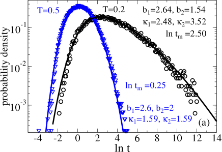
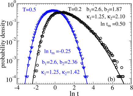
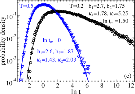
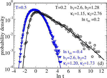
Figure 6: (Color online) Probability density function of log-transformed first escape times from the interval $[-\lambda,\lambda]$ for two temperatures $T=0.5$ (in blue) and $T=0.2$ (in black). The cases in the different panels are (a) exponential correlations, (b) power-law correlations with $\gamma=0.8$, (c) linearly decaying correlations, and (d) Gaussian correlation decay. The symbols represent simulations data, the lines correspond to a fit with the probability density (13). Parameters are shown in the panels. With decreasing temperature the distributions become broader and the parameter $b_{2}$ smaller.

All moments of the corresponding residence time distribution in any finite spatial domain are finite. Moreover, the average residence time is much (for $k_{B}T\ll\sigma$ orders of magnitude) smaller than the one expected from the normal diffusion characterized the renormalized result $D_{\rm ren}$ Goychuk and Kharchenko (2014). In the present case, weak ergodicity breaking does not rely on infinite mean residence times, what makes it especially interesting in biological applications. Residence time distributions of escape times for particles initially located in the center of a symmetric interval $\pm\lambda$ in space for $k_{B}T\leq 0.5\sigma$ are nicely described by a generalized log-normal distribution reading

$$\psi(t) = \frac{C}{t}\Big{[}e^{-|\ln(t/t_{m})/\kappa_{1}|^{b_{1}}}\theta(t_{m}-t)$$ (13)

$$+e^{-|\ln(t/t_{m})/\kappa_{2}|^{b_{2}}}\theta(t-t_{m})\Big{]},$$

where $C=b_{1}b_{2}/[b_{2}\kappa_{1}\Gamma(1/b_{1})+b_{1}\kappa_{2}\Gamma(1/b_{2})]$ is a renormalization constant, $b_{1,2}>1$, and $\kappa_{1,2}>0$. $\Gamma(x)$ denotes the complete Gamma function. For any $b_{1,2}>1$, this distribution (13) has finite moments $\langle t^{n}\rangle$ of all orders $n$. For $b_{1}=b_{2}=2$ and $\kappa_{1}=\kappa_{2}$, this is the well-known log-normal distribution. However, in our case $b_{1}$ and $b_{2}$ are different, and $\kappa_{1}\neq\kappa_{2}$. Namely, for the exponential correlations $b_{1}\approx 2.6\div 2.7$, and it is weakly temperature dependent. However, $b_{2}$ does depend visibly on temperature. For $T=0.5$, $b_{2}=2$, and it becomes smaller with decreasing temperature while $t_{m}$ becomes longer. For instance, for $T=0.2$, $b_{2}\approx 1.54$, see Fig. 6a, where the distribution of times is plotted for the log-transformed variable $\ln t$, attaining a maximum at $\ln t_{m}$.

III.2 Power law correlations

We proceed with the case of power law correlations of the spatial potential fluctuations, with $\gamma=0.8$. The ensemble averages for the mean squared displacement are depicted in Fig. 2c. Here, the fit with $\delta=1$ works generally better, which can be rationalized from Fig. 1, and for $T=0.1$ a generalized Sinai diffusion with $a\approx 3$ nicely fits the numerical data over six decades in time. Note in Fig. 3b that $\alpha(t)$ stays nearly constant over five decades in time, up to the end of the simulations even for $T=1/3$. For the larger $T=0.5$, it also grows logarithmically in time, as in the case of exponential correlations. Why $\alpha(t)$ changes slower in time in this case and a fit with $\delta=1$ and $\sigma_{\rm eff}\approx 1.41$ works nicely over many time decades for intermediate temperatures can be rationalized from the fact that the non-ergodicity length $L_{\rm erg}$ in this case is much larger, see Table 1. The case of power law correlations is especially important for the diffusion of regulatory proteins on DNA strands, where such long-range correlations with $\gamma\sim 0.6\div 0.8$ emerge due to the way biological information is encoded in the base pair sequence. Our results imply that such diffusion should be typically anomalously slow with $\alpha\sim 1.41\;k_{B}T/\sigma$ in the corresponding range of temperatures, for $\gamma=0.8$. It must be stressed in this respect that diffusion does not become immediately normal for $\langle\delta x^{2}(t)\rangle>L_{\rm erg}^{2}$, but rather a very slow crossover with growing $\alpha(t)$ emerges, see Fig. 2c for $T=0.5$. Here, the transition to the asymptotic regime of normal diffusion is still far from being established.

Somewhat surprisingly, for power law correlations subdiffusion is essentially faster in absolute terms than in the case of exponentially short correlations, see Fig. 7. This may first appear counter-intuitive. However, one reason for this feature becomes clear from the potential fluctuations depicted in Fig. 1, which for the exponential correlations are essentially larger (thinking in units of $k_{B}T$). Clearly, exponential correlations and other singular (in the limit $\Delta x\to 0$) models of static disorder present a preferred case to observe Sinai type diffusion in such systems. The second explanation is that in the case of power law correlations a local bias is present on a much longer scale. This leads to an essential acceleration of diffusion in the ensemble sense, see Fig. 5b, where the ensemble mean squared displacement is in fact superdiffusive (see also Fig. 3b for the initial regime) within several correlation lengths at $T=0.2$. Remarkably, it is even faster than the potential free diffusion. This is namely due to the presence a local bias, which is also the reason for the Golosov phenomenon in Sinai diffusion. The single trajectory time averaged mean squared displacement, however, does not show such a striking feature, see Fig. 5b. The reasoning for this feature is that the local bias is averaged out in the single trajectory time averaging for a sufficiently large measurement time $T_{\rm w}$. Single trajectory averages spread out slower than the ensemble averaged result and, nevertheless, their broadening is many orders of magnitude faster than the result of the renormalized normal diffusion. This is why even for $\sigma\sim 4\div 5$, relevant for some important biophysical situations Gerland et al. (2002); Lässig (2007), regulatory proteins can diffuse on DNA tracks despite of the fact that the classical de Gennes-Zwanzig-Bässler result would predict that they should be practically localized (on biophysically relevant time scales) for such a strong disorder. Naturally, single trajectory averages exhibit a large scatter due to a transient lack of ergodicity. It is important to mention that a strong single trajectory scatter was indeed observed experimentally Wang et al. (2006). Note also that such a local bias can be functionally very important, directing the protein toward a specific binding site on DNA. The ensemble averaged time averaged mean squared displacement in this case also shows a power law scaling in time, see Fig. 5b. Judging from the power law exponent $\alpha_{\rm EATA}=0.31$, it appears to be slower than in the case of exponential correlations, where $\alpha_{\rm EATA}=0.54$, compare with Fig. 5a. However, the prefactor in this case is, in fact, much larger, which makes it in fact faster rather than slower.

The distribution of escape times is also nicely captured by the generalized log-normal distribution (13), as seen in Fig. 6b. Note that the escape times in this case are essentially shorter than in the case of exponential correlations, Fig. 6a. Particularly, the scaling exponent $b_{2}$ is larger and the half width $\kappa_{2}$ is smaller. Conversely, the power exponent $b_{1}$ is pretty robust, $b_{1}\sim 2.6$ (also for other models of disorder, see below).

III.3 Linear correlations

The case of linear correlations presents another important model of singular disorder with potential fluctuations growing with diminishing $\Delta x$. Therefore, it is expected to be similar to the case of exponential correlations, despite the fundamental difference between these two models. The non-ergodicity length $L_{\rm erg}$ here is the shortest within the four considered models, see Table 1. The ensemble averaged mean squared displacement is depicted in Fig. 2d. Qualitatively, it appears very similar to the previous cases, however, it turns out to be the slowest one, as Fig. 7 reveals. In this case, $\sigma_{\rm eff}\sim 4.22\div 4.91$, and $x_{\rm in}\sim 0.27\div 0.67$, except from $T=0.1$, where $x_{\rm in}\approx 3.65$. Now, the agreement with $x_{0}\approx 0.314$ is much better. It might seem paradoxical that the shortest correlations, which exactly vanish at distances exceeding $\lambda$, yield the slowest diffusion. However, it must be kept in mind that in the absence of spatial correlation we have just normal diffusion, which is orders of magnitude slower than the considered correlation-induced subdiffusion. The time behavior of the anomalous diffusion exponent $\alpha(t)$ is indeed more similar to the one in the case of exponential correlations than to the case of power law correlations, see Fig. 3c, and compare with panels (a) and (b) therein. The scatter of the single trajectory time averaged mean squared displacements is also quite pronounced, see Fig. 5c. The escape times obey the same distribution (13), as depicted in Fig. 6c, but with different parameters. Similar to previous cases, $b_{1}\sim 2.6\div 2.7$, nearly independent of temperature, while $b_{2}$ strongly depends on temperature, decreasing with decreasing temperature. All temporal moments of the resident times remain, however, finite with decreasing temperature.

III.4 Gaussian correlations

Finally, we consider the case of Gaussian spatial correlations. Judging from Fig. 1 it should be the second fastest of the four models considered here. This is indeed the case, as seen in Fig. 7. The ensemble averaged mean squared displacements display very similar generic features as in the other cases, see Fig. 2e. Here, $\sigma_{\rm eff}\sim 4.50\div 5.10$ and $x_{\rm in}\sim 0.41\div 4.70$, whereas the theoretical is $x_{0}\approx 2.22$. Once again, the discrepancy by a factor of less than two with the theoretical $\sigma_{\rm eff}=2.83$, and at least the correct order of magnitude for $x_{\rm in}$ are quite impressive, given the simplicity of our scaling argumentation. Sinai type diffusion with $a=4$ is featured in the low temperature behavior at $T=0.1$. In this case, however, $\alpha(t)$ already starts to slightly increase at the end of the simulations already at $T=0.1$, Fig. 3d. This type of correlations indeed presents the worst case to observe a Sinai like diffusion. The reasons are quite obvious: Namely, (1) this model of disorder is not singular and (2) the correlations are short-ranged. Single trajectory averages of the mean squared displacement are strongly scattered, and their ensemble average yields a power law dependence for sufficiently large times, Fig. 5d. Finally, the distribution of the escape times obeys the same common pattern, as seen in Fig. 6d.

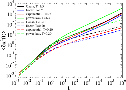
Figure 7: (Color online) Comparison of the ensemble-averaged mean squared displacement for the four different models of the correlation decay and for two values of temperature. Seemingly against intuition, the mean squared displacement is the largest in the case of power-law spatial correlations, where the spatial non-ergodicity scale is the longest. Moreover, diffusion is slowest in the case of linear correlations, where the non-ergodicity length is the shortest in all four cases, see Table 1.

IV Discussion and conclusions

Diffusion in systems characterized by Gaussian fluctuations of the potential with spatially decaying correlations is typically thought of as normally diffusive on experimentally relevant time scales, following the renormalization idea for these systems developed by de Gennes, Zwanzig, and Bässler. Following recent discoveries of extended anomalous diffusion in such systems, we here provided a clear physical picture for the origin of subdiffusion in stationary Gaussian random potentials with decaying spatial correlations. While the anomalous diffusion is, of course, transient, the scaling theory developed and confirmed herein demonstrates that this transient may easily reach macroscopic time scales for a physically relevant strength of the potential fluctuations.

The primary reason for the origin of this subdiffusion is that the maximal amplitude of the potential fluctuations grows logarithmically with the distance, in accordance with the asymptotic theoretical result (1) and the simulations data depicted in Fig. 1. This behavior is universal, and it has a predictive power. In particular, it allows to predict for which model of the potential correlations decay the anomalous diffusion will be faster in absolute terms—and this prediction completely agrees with numerics. The strongest trapping effects leading to anomalous diffusion occur in the case of singular models of disorder, such as exponential or linear decays of the correlations, for which the stationary energy autocorrelation function is not differentiable at the origin. This leads to unbounded static force root mean squared fluctuations $\langle f^{2}\rangle^{1/2}\to\infty$ in the strict $\Delta x\to 0$ limit of the coarse graining. Strictly speaking, such models are not amenable to any Langevin simulations unless the random potential is considered on a lattice with a spatial grid $\Delta x$, as incorporated in our simulations, with discrete potential points connected by parabolic splines (locally piece-wise linear forces). A maximal time step of the Langevin simulations must be chosen accordingly, depending on $\Delta x$ and the averaged local force root mean square $\langle f^{2}\rangle^{1/2}$. Singular disorder models are regularized accordingly. However, they display the largest potential fluctuations in Fig. 1.

Spatially increasing potential fluctuations may appear strange and contradictory to the very fact that the random potential is stationary and possesses the well defined root mean squared magnitude $\sigma$. This property of continuous albeit logarithmic increase with distance is, however, the very cornerstone of the theory of extreme events Castillo et al. (2004): An extreme event will always occur, if only one waits sufficiently long, and even if the probability density of such events is strongly localized such as in the case of the considered Gaussian distribution. In our case, the extreme events occur in space rather than time, but have the same origin. The law (1) of potential fluctuations with a $(\log x)^{\delta}$ scaling ($\delta=1/2$) is valid asymptotically. The longer the spatial correlations of the potential fluctuations reach, the later this asymptotic is achieved. Numerically, we also observed different scaling exponents such as $\delta=1$ transiently and $\delta>1$ initially.

Based on these observations we put forward a very simple scaling theory of anomalous diffusion in the potential landscape $U(x)$, which in essence is very similar to the scaling theory of Sinai diffusion developed in the classical Ref. Bouchaud and Georges (1990). It leads to our major result given in Eq. (3) and explains why for sufficiently low temperatures we indeed observe a generalized Sinai diffusion with a power law exponent, which is generally different from $a=4$ and can be even smaller as shown in Figs. 2b, c, and d: The diffusion is formally even slower than for the case of Sinai diffusion in random force fields. Our analytical results were shown to be valid over five to seven decades in time, at least, which is a remarkable success of the relatively simple scaling approach. The nominally ultraslow diffusion is in fact many orders of magnitude faster than the asymptotical limit of the disorder-renormalized normal diffusion, which for the physically relevant parameters considered here simply cannot be attained neither physically nor numerically for such a strong disorder. Hence, it becomes completely irrelevant in such settings. This provides a striking example of how the formally valid mathematical result of asymptotic, disorder-renormalized normal diffusion in the de Gennes-Zwanzig-and Bässler theory may produce physically inappropriate descriptions on meso- and macroscales.

This result also leads to a number of further predictions, which are confirmed in numerical simulations and agree with previous simulations of the considered stochastic dynamics in random potentials. Namely, this kind of anomalous diffusion is generally characterized by a time dependent power law exponent $\alpha(t)$, for which we obtained the theoretical result (6). This result predicts that, after an initial decay ($\delta>1$), the anomalous diffusion exponent $\alpha(t)$ will reach a minimum for which $\alpha_{\rm min}=2k_{B}T/\sigma_{\rm eff}$ (for $\delta=1$) and then gradually grow in logarithmic fashion, $\alpha(t)=2(k_{B}T/\sigma_{\rm eff})^{2}\ln(t/t_{0})$ ($\delta=1/2$). These two nontrivial predictions are remarkably well confirmed by extensive numerical simulations. Indeed, $\alpha_{\rm min}=2k_{B}T/\sigma_{\rm eff}$ with $\sigma_{\rm eff}\sim 1.24\div 1.52$, within a broad range of temperatures, as demonstrated in Fig. 3. Moreover, at sufficiently large temperatures, $\alpha(t)$ indeed grows logarithmically, see Fig. 3. It is indeed remarkable how a simple scaling theory can be predictive to such a degree. Of course, the scaling results cannot be fully accurate on a quantitative level and claim full consistency over the entire range of parameters and times studied herein. In particular, the values of $\sigma_{\rm eff}$ and $t_{0}$ used to fit the numerical data, for instance, in Figs. 2 and 3 are in fact different. This is due to the fact that the approximation of Eq. (3) by Eqs. (5) and (6) is, indeed, a bit too coarse. Nevertheless, the coherence and validity of our scaling theoretical predictions are compelling.

We note that in the biologically relevant and important case of power law decaying correlations the scaling $\delta=1$ applies to a much larger range of times and temperatures, as shown in Figs. 2c and 3b. In this case, power law subdiffusion of the form $\langle\delta x^{2}(t)\rangle\propto t^{\alpha}$ with $\alpha\approx 1.41\;k_{B}T/\sigma$ in fact presents a good approximation over a broad range of times and temperatures. This behavior may easily be confused with the law $\alpha\approx k_{B}T/\sigma$ produced by the mean field continuous time random walk with exponential energy disorder Hughes (1995); ben Avraham and Havlin (2000); Metzler and Klafter (2000). In striking contrast to the latter model, however, the residence times in a finite spatial domain are not power-law distributed but follow the generalized log-normal distribution (13) shown in Fig. 6, for all the studied models of the correlation decay. All moments of this distribution are finite, which is a very attractive physical feature. This subdiffusion is clearly non-ergodic, as it is demonstrated in Fig. 5, where the maximal time is merely $1\%$ of the time window $T_{\rm w}$ used to accumulate the single-trajectory averages. Hence, a large scatter is a truly non-ergodic effect, even if it is a transient one and must vanish in the mathematical limit $T_{\rm w}\to\infty$ Goychuk and Kharchenko (2014). It is, however, not necessarily attainable experimentally.

The origin of this lack of ergodicity was already explained in Ref. Goychuk and Kharchenko (2014): It is due to the absence of self-averaging of the statistical weight function $w(x)=\exp[\pm\beta U(x)]$ on the spatial scale $L_{\rm erg}$, implicitly defined in relation (7), depending on the disorder autocorrelation function $g(x)$. Solving this equation analytically in the case of linearly decaying correlations yields the exact result (8) and a very handy and highly accurate approximate result in Eq. (9). In this case of linear decay, $L_{\rm erg}$ turns out to be the shortest one within all models of $g(x)$ considered in this paper, see Table 1. This result implies that $L_{\rm erg}$ in units of the correlation scale $\lambda$ is only by a factor $(1/2)(\sigma/k_{B}T)^{2}$ smaller than the factor $\exp[\sigma^{2}/(k_{B}T)^{2}]$ suppressing the asymptotically normal diffusion coefficient in the renormalization sense. This, in turn, means that such mesoscopic subdiffusion can readily reach macroscopic scales even for a moderate disorder strength $\sigma\sim 4\div 5\;k_{B}T$ featuring many physical and biological systems already at room temperatures.

Different from the annealed continuous time random walk subdiffusion, the single trajectory time averages for the mean squared displacement in the present case of quenched potential fluctuations are characterized by different power law exponents $\alpha\neq 1$ Goychuk and Kharchenko (2014), and not just a linear scaling with the lag time (erroneously suggesting normal diffusion) but with a significantly scattered diffusion coefficient Lubelski et al. (2008); He et al. (2008). Importantly, especially with respect to biological applications is that the subdiffusion considered here is in fact orders of magnitude faster than the normal diffusion predicted by the classical renormalization result with effective diffusivity $D_{\rm ren}$. For example, for the diffusion of regulatory proteins on DNA tracks, $\sigma\approx 4.3\;k_{B}T_{\rm room}$, which can be deduced from the results presented in Ref. Lässig (2007). Hence, $D_{\rm ren}=9.33\times 10^{-9}D_{0}$, and for a typical experimental value $D_{0}=3\;\mu{\rm m^{2}/s}$ Elf et al. (2007) it would become $D_{\rm ren}\approx 2.8\times 10^{-2}{\rm nm^{2}/s}$. This would mean that within some hundreds of seconds the diffusional spread would be merely several nanometers. However, this renormalization result underestimates massively, on the relevant time scales of this phenomenon, the actual protein mobility. Our results demonstrate that the actually occurring subdiffusion is orders of magnitude faster than one suggested by this normal diffusion result of the renormalization approach. Hence, correlations-induced persistent subdiffusion makes diffusional search feasible in such a situation despite a strong binding-energy disorder.

An important role in applications may also be played by the presence of a local bias, which is especially clearly expressed in the case of power law correlations. This is the analogous reason for the Golosov phenomenon in the case of random potential exhibiting Brownian motion in space Bouchaud and Georges (1990). Then, the particles which were initially localized nearby diffuse similarly, in a correlated fashion. The distance between them does not grow dramatically in time, being bounded. One can find similar single trajectory averages also in our numerical results. Conversely, different particles starting in locally different environments can move into opposite directions, and this can give rise to an enhanced diffusivity in the ensemble sense. In fact, due to this reason an initial regime of superdiffusion can be realized in Fig. 5b and d on the ensemble level in the case of power-law correlations, for which it can extend over several scaling lengths $\lambda$, see also Fig. 3b and d for small times. In the case of single trajectory time averages, the local bias averages out. Therefore, such a superdiffusive regime is absent. Diffusion on the level of single trajectories is typically slower than the one on the ensemble level, see, for instance, Fig. 5. The difference between the ensemble average and the ensemble-averaged time average of the mean squared displacement becomes smaller with increasing time. The latter ensemble-time-averages display a power law dependence on time for sufficiently large times even in the Sinai like regime on the ensemble level, which can be an important observation with respect to possible experimental manifestations.

To conclude, we elucidated the physical mechanism leading to subdiffusion in stationary correlated potentials with spatially decorrelating Gaussian disorder, and we showed that a generalized Sinai diffusion typically emerges at sufficiently low temperatures and/or strong disorder for various models of decaying correlations. Our scaling theory also explains how a standard power law subdiffusion emerges with increasing temperature and in the course of time. Such subdiffusion is weakly non-ergodic, displays a local bias and proceeds much faster than de Gennes-Bässler-Zwanzig limit of normal diffusion, which for sufficiently low temperatures and/or finite size of the system simply cannot be attained physically on typical mesoscales. We believe that our results provide a new vista on the old problem of potential disorder, and that they will be very useful in the context of non-ergodic diffusion processes, especially in relation to various biologically relevant problems on the cellular level. Likely they are also important for diffusion of colloidal particles in laser created random potentials, a conjecture calling for further experimental studies of such systems.

References

- Bouchaud and Georges (1990) J.-P. Bouchaud and A. Georges, Anomalous diffusion in disordered media: Statistical mechanisms, models and physical applications, Phys. Rep. 195, 127 (1990).
- Bouchaud et al. (1990) J. Bouchaud, A. Comtet, A. Georges, and P. L. Doussal, Classical diffusion of a particle in a one- dimensional random force field, Ann. Phys. (N.Y.) 201, 285 (1990).
- Bässler (1993) H. Bässler, Charge transport in disordered organic photoconductors: a Monte Carlo simulation study, Phys. Status Solidi B 175, 15 (1993).
- Dunlap et al. (1996) D. H. Dunlap, P. E. Parris, and V. M. Kenkre, Charge-dipole model for the universal field dependence of mobilities in molecularly doped polymers, Phys. Rev. Lett. 77, 542 (1996).
- Bässler (1987) H. Bässler, Viscous flow in supercooled liquids analyzed in terms of transport theory for random media with energetic disorder, Phys. Rev. Lett. 58, 767 (1987).
- Gerland et al. (2002) U. Gerland, J. D. Moroz, and T. Hwa, Physical constraints and functional characteristics of transcription factor-DNA interaction, Proc. Natl. Acad. Sci. (USA) 99, 12015 (2002).
- Lässig (2007) M. Lässig, From biophysics to evolutionary genetics: Statistical aspects of gene regulation, BMC Bioinformatics 8(Suppl. 6), S7 (2007).
- Slutsky et al. (2004) M. Slutsky, M. Kardar, and L. A. Mirny, Diffusion in correlated random potentials, with applications to DNA, Phys. Rev. E 69, 061903 (2004).
- Evers et al. (2013) F. Evers, R. D. L. Hanes, C. Zunke, R. F. Capellmann, J. Bewerunge, C. Dalle-Ferrier, M. C. Jenkins, I. Ladadwa, A. Heuer, R. Castaneda-Priego, and S. U. Egelhaaf, Colloids in light fields: particle dynamics in random and periodic energy landscapes, Eur. Phys. J. Spec. Top. 222, 2995 (2013).
- Hanes and Egelhaaf (2012) R. D. L. Hanes and S. U. Egelhaaf, Dynamics of individual colloidal particles in one-dimensional random potentials: a simulation study, Journal of Physics: Condensed Matter 24, 464116 (2012).
- Hanes et al. (2013) R. D. L. Hanes, M. Schmiedeberg, and S. U. Egelhaaf, Brownian particles on rough substrates: relation between intermediate subdiffusion and asymptotic long-time diffusion, Phys. Rev. E 88, 062133 (2013).
- Bewerunge and Egelhaaf (2016) J. Bewerunge and S. U. Egelhaaf, Experimental creation and characterization of random potential-energy landscapes exploiting speckle patterns, Phys. Rev. A 93, 013806 (2016).
- Hänggi et al. (1990) P. Hänggi, P. Talkner, and M. Borkovec, Reaction-rate theory: fifty years after Kramers, Rev. Mod. Phys. 62, 251 (1990).
- Gennes (1975) P. G. D. Gennes, Brownian motion of a classical particle through potential barriers. application to the helix-coil transitions of heteropolymers, J. Stat. Phys. 12, 463 (1975).
- Zwanzig (1988) R. Zwanzig, Diffusion in a rough potential, Proc. Natl. Acad. Sci. (USA) 85, 2029 (1988).
- Hecksher et al. (2008) T. Hecksher, A. I. Nielsen, N. B. Olsen, and J. C. Dyre, Little evidence for dynamic divergences in ultraviscous molecular liquids, Nat. Phys. 4, 737 (2008).
- Romero and Sancho (1998) A. H. Romero and J. M. Sancho, Brownian motion in short range random potentials, Phys. Rev. E 58, 2833 (1998).
- Hughes (1995) B. D. Hughes, Random Walks and Random Environments (Clarendon Press, Oxford, 1995).
- Metzler and Klafter (2000) R. Metzler and J. Klafter, The random walk’s guide to anomalous diffusion: a fractional dynamics approach, Phys. Rep. 339, 1 (2000).
- Schubert et al. (2013) M. Schubert, E. Preis, J. C. Blakesley, P. Pingel, U. Scherf, and D. Neher, Mobility relaxation and electron trapping in a donor/acceptor copolymer, Phys. Rev. B 87, 024203 (2013).
- Scher and Montroll (1975) H. Scher and E. W. Montroll, Anomalous transit-time dispersion in amorphous solids, Phys. Rev. B 12, 2455 (1975).
- Goychuk and Kharchenko (2014) I. Goychuk and V. O. Kharchenko, Anomalous features of diffusion in corrugated potentials with spatial correlations: faster than normal, and other surprises, Phys. Rev. Lett. 113, 100601 (2014).
- Peng et al. (1992) C.-K. Peng, S. V. Buldyrev, A. L. Goldberger, S. Havlin, F. Sciortino, M. Simons, and H. E. Stanley, Long-range correlations in nucleotide sequences, Nature (London) 356, 168 (1992).
- ben Avraham and Havlin (2000) D. ben Avraham and S. Havlin, Diffusion and Reactions in Fractals and Disordered Systems (Cambridge University Press, Cambridge, 2000).
- Khoury et al. (2011) M. Khoury, A. M. Lacasta, J. M. Sancho, and K. Lindenberg, Weak disorder: anomalous transport and diffusion are normal yet again, Phys. Rev. Lett. 106, 090602 (2011).
- Simon et al. (2013) M. S. Simon, J. M. Sancho, and K. Lindenberg, Transport and diffusion of overdamped Brownian particles in random potentials, Phys. Rev. E 88, 062105 (2013).
- Bouchaud (1992) J. P. Bouchaud, Weak ergodicity breaking and aging in disordered systems, J. Phys. I (Paris) 2, 1705 (1992).
- Bel and Barkai (2005) G. Bel and E. Barkai, Weak ergodicity breaking in the continuous-time random walk, Phys. Rev. Lett. 94, 240602 (2005).
- Metzler et al. (2014) R. Metzler, J.-H. Jeon, A. G. Cherstvy, and E. Barkai, Anomalous diffusion models and their properties: non-stationarity, non-ergodicity, and ageing at the centenary of single particle tracking, Phys. Chem. Chem. Phys. 16, 24128 (2014).
- Burov and Barkai (2007) S. Burov and E. Barkai, Occupation time statistics in the quenched trap model, Phys. Rev. Lett. 98, 250601 (2007).
- Lubelski et al. (2008) A. Lubelski, I. M. Sokolov, and J. Klafter, Nonergodicity mimics inhomogeneity in single particle tracking, Phys. Rev. Lett. 100, 250602 (2008).
- He et al. (2008) Y. He, S. Burov, R. Metzler, and E. Barkai, Random time-scale invariant diffusion and transport coefficients, Phys. Rev. Lett. 101, 058101 (2008).
- Sokolov et al. (2009) I. Sokolov, E. Heinsalu, P. Hänggi, and I. Goychuk, Universal fluctuations in subdiffusive transport, Europhys. Lett. 86, 30009 (2009).
- Wang et al. (2006) Y. M. Wang, R. H. Austin, and E. C. Cox, Single molecule measurements of repressor protein 1d diffusion on DNA, Phys. Rev. Lett. 97, 048302 (2006).
- Sinai (1982) Y. G. Sinai, The limiting behavior of a one-dimensional random walk in random medium, Theor. Prob. Appl. 27, 247 (1982).
- Le Doussal et al. (1999) P. Le Doussal, C. Monthus, and D. S. Fisher, Random walkers in one-dimensional random environments: exact renormalization group analysis, Phys. Rev. E 59, 4795 (1999).
- Godec et al. (2014) A. Godec, A. V. Chechkin, E. Barkai, H. Kantz, and R. Metzler, Localisation and universal fluctuations in ultraslow diffusion processes, J. Phys. A 47, 492002 (2014).
- Oshanin et al. (2013) G. Oshanin, A. Rosso, and G. Schehr, Anomalous fluctuations of currents in sinai-type random chains with strongly correlated disorder, Phys. Rev. Lett. 110, 100602 (2013).
- Castillo et al. (2004) E. Castillo, A. S. Hadi, N. Balakrishnan, and J. M. Sarabia, Extreme Value and Related Models with Applications in Engineering and Science (John Wiley & Sons, Hoboken, 2004).
- Pickands (1969) J. Pickands, Upcrossing probabilities for stationary gaussian processes, Trans. Amer. Math. Soc. 145, 51 (1969).
- Zhang (1986) Y. C. Zhang, Diffusion in a random potential: hopping as a dynamical consequence of localization, Phys. Rev. Lett. 56, 2113 (1986).
- Papoulis (1991) A. Papoulis, Probability, Random Variables, and Stochastic Processes, 3rd ed. (McGraw-Hill Book Company, New York, 1991).
- Bénichou et al. (2009) O. Bénichou, Y. Kafri, M. Sheinman, and R. Voituriez, Searching fast for a target on DNA without falling to traps, Phys. Rev. Lett. 103, 138102 (2009).
- Bauer et al. (2015) M. Bauer, E. S. Rasmussen, M. A. Lomholt, and R. Metzler, Real sequence effects on the search dynamics of transcription factors on DNA, Sci. Rep. 5, 10072 (2015).
- Simon et al. (2012) M. S. Simon, J. M. Sancho, and A. M. Lacasta, On generating random potentials, Fluct. Noise Lett. 11, 1250026 (2012).
- Stewart et al. (2012) A. J. Stewart, S. Hannenhalli, and J. B. Plotkin, Why transcription factor binding sites are ten nucleotides long, Genetics 192, 973 (2012).
- Yaglom (1972) A. M. Yaglom, An Introduction to the Theory of Stationary Random Functions (Dover Publications, New York, 1972).
- Golosov (1984) A. O. Golosov, Localization of random walks in one-dimensional random environments, Commun. Math. Phys. 92, 491 (1984).
- Elf et al. (2007) J. Elf, G.-W. Li, and X. S. Xie, Probing transcription factor dynamics at the single-molecule level in a living cell, Science 316, 1191 (2007).