Automated adjoints of coupled PDE-ODE systems

Abstract

Mathematical models that couple partial differential equations (PDEs) and spatially distributed ordinary differential equations (ODEs) arise in biology, medicine, chemistry and many other fields. In this paper we discuss an extension to the FEniCS finite element software for expressing and efficiently solving such coupled systems. Given an ODE described using an augmentation of the Unified Form Language (UFL) and a discretisation described by an arbitrary Butcher tableau, efficient code is automatically generated for the parallel solution of the ODE. The high-level description of the solution algorithm also facilitates the automatic derivation of the adjoint and tangent linearization of coupled PDE-ODE solvers. We demonstrate the capabilities of the approach on examples from cardiac electrophysiology and mitochondrial swelling.

65L06, 65M60, 65M32, 35Q92

1 Introduction

In this paper we discuss solvers for systems involving spatially dependent ordinary differential equations (ODEs) of the following form: given an initial condition $y_{0}(x)$, find $y=y(x,t)$ such that

(1) $${y}_{t}(x,t)=f(y,x,t),\quad y(x,t_{0})=y_{0}(x),$$

for all $x$ in a point set $X\subset\Omega\subseteq\mathbb{R}^{d}$, where $d$ is the spatial dimension. The subscript $t$ refers to differentiation in time. The right-hand side $f$ cannot depend on spatial derivatives of $y$; the ODE is decoupled at different points. Problems of this form often arise when discretizing time-dependent mathematical models that couple PDEs with spatially distributed systems of ODEs via operator splitting. Examples of application areas include cardiac electrophysiology in general [27, 20] and cardiac ion channel modeling in particular [11], mitochondrial swelling [8], groundwater flow and contamination [30], pulmonary gas transport [31, 6], and plasma-enhanced chemical vapor deposition [12]. We also discuss the automated derivation of the adjoint and tangent linearization of such models: these can be used to identify the sensitivity of the solution to model parameters, solve inverse problems for unknown parameters, and characterize the stability of trajectories.

For concreteness, we present two biological examples of coupled PDE-ODE systems where problems of the form (1) arise. We return to numerical results for these examples in Section 6.

Example 1 (The bidomain equations).

As our first motivating example, we will consider the bidomain equations for the propagation of an electrical signal in a non-deforming domain $\Omega$ [27]: find the transmembrane potential $v=v(x,t)$, the extracellular potential $u_{e}(x,t)$ and additional state variables $s=s(x,t)$ such that for $t\in(0,T]$:

(2a) $${v}_{t}-\operatorname{div}(M_{i}\operatorname{grad}v+M_{i}\operatorname{grad}u_{e}) =-I_{\rm ion}(v,s)+I_{s} \text{in }\Omega,$$

(2b) $$-\operatorname{div}\left(M_{i}\operatorname{grad}v+(M_{i}+M_{e})\operatorname{grad}u_{e}\right) =0 \text{in }\Omega,$$

(2c) $${s}_{t} =F(v,s) \forall x\in\Omega.$$

In (2), $I_{\rm ion}$ is a given nonlinear function describing ionic currents and $F$ defines a system of nonlinear functions, while $M_{i}$ and $M_{e}$ are the intracellular and extracellular conductivity tensors, respectively, and $I_{s}$ is a given stimulus current. The function $F$ cannot depend on spatial derivatives of $v$ and $s$; it defines a pointwise system of ODEs. The specific form of $I_{\rm ion}$ and $F$ are typically prescribed by a given cardiac cell model and may vary greatly in complexity: from involving a single state variable $s$ such as the FitzHugh-Nagumo model [11] to models with e.g. $41$ state variables such as the model of O’Hara et al. [21]. The system (2) is closed with appropriate initial and boundary conditions. After the application of operator splitting, the ODE step is decoupled from the PDE step and is a system of the form of (1).

Example 2 (Mitochondrial swelling).

As a second example, we consider a model proposed in [8] to describe the swelling of mitochondria. Mitochondrial swelling plays a key role in the process of programmed cell death (apoptosis) and thus for the life cycle of cells. Mathematically, we consider the following model [8, p. 26]: find the calcium concentration $u=u(x,t)$ and the densities of mitochondria states $N_{i}=N_{i}(x,t)$ for $i=1,2,3$ such that

(3a) $${u}_{t} =d_{1}\Delta(|u|^{q-2}u)+d_{2}g(u)N_{2} \text{in }\Omega,$$

(3b) $${N_{1}}_{t} =-f(u)N_{1} \forall x\in\Omega,$$

(3c) $${N_{2}}_{t} =f(u)N_{1}-g(u)N_{2} \forall x\in\Omega,$$

(3d) $${N_{3}}_{t} =-g(u)N_{2} \forall x\in\Omega.$$

where $d_{1}\geq$ is a diffusion coefficient, $d_{2}\geq 0$ is a feedback parameter, $q\geq 2\in\mathbb{N}$ determines the nonlinearity of the diffusion-type operator, and $g$ and $f$ are prescribed functions. The functions $N_{1}$, $N_{2}$ and $N_{3}$ describe the densities of unswollen, swelling and completely swollen mitochondria respectively. Equation (3a) is a spatially-coupled PDE, while equations (3b)-(3d) define pointwise ODEs. The system is closed with initial conditions and Dirichlet boundary conditions for $u$. Again, after operator splitting, a subproblem of the form (1) results.

Over the last decade, there has been a growing interest in computational frameworks for the rapid development of numerical solvers for PDEs such as the FEniCS Project [16], the Firedrake Project [23], and Feel++ [22]. The rapid development of solvers is achieved by offering high-level abstractions for the expression of such problems. Each of these projects provides a domain-specific language for specifying finite element variational formulations of PDEs and associated software for their efficient solution. The methods presented in this paper are implemented in the the FEniCS Project and dolfin-adjoint [10]; dolfin-adjoint automatically derives discrete adjoint and tangent linear models from a FEniCS forward model. These allow for the efficient computation of functional gradients and Hessian-vector products, and are essential ingredients in stability analyses, parameter identification and inverse problems.

However, these systems do not currently efficiently extend to the kind of coupled PDE-ODE systems arising in computational biology. While monolithic finite element discretizations of coupled PDE-ODE systems such as (2) or (3) may easily be specified and solved using the current software features in FEniCS, this approach will involve an unreasonably large computational expense, as the monolithic system is highly nonlinear and the solver cannot exploit the fact that the ODE is spatially decoupled.

Operator splitting is the method of choice for such coupled PDE-ODE systems [27], and is implemented as standard in many hand-written codes, see e.g. [29, 19] in the context of cardiac electrophysiology. Operator splitting decouples a PDE-ODE system into a spatially-coupled system of PDEs and a spatially-decoupled collection of ODE systems. This collection of ODE systems then typically takes the form (1), which can be solved using well-known temporal discretization methods. Heretofore it has not been possible to specify spatially-decoupled ODE systems in high-level PDE frameworks such as the FEniCS or Firedrake projects.

This work addresses the gap in available abstractions, algorithms and software for arbitrary PDE-ODE systems. We introduce high-level domain-specific language constructs for specifying collections of ODE systems and for specifying multistage ODE schemes via Butcher tableaux. This has several major benefits. By automatically generating the solver from a high-level description of the problem, practitioners can flexibly explore a range of models; this is especially important in biological problems where the model itself is uncertain. Another advantage is that a high-level description facilitates the automated derivation of the associated tangent linear and adjoint models. This represents a significant saving in the time taken to investigate questions of biological interest.

The main new contributions of this paper are (i) the extension of the FEniCS finite element system to enable efficient the large-scale forward solution of coupled, time-dependent PDE-ODE systems via operator splitting, and (ii) the extension of dolfin-adjoint to automatically derive and solve the associated tangent linear and adjoint models, enabling efficient automated computation of functional gradients for use in e.g. optimization or adjoint-based sensitivity analysis.

This paper is organized as follows. In Section 2, we describe the general operator splitting setting, the resulting separate PDE and ODE systems, and natural discretizations of these. We continue in Section 3 by briefly describing the well-established ODE schemes that we consider in this work: the multistage and Rush-Larsen families. We discuss the adjoint and tangent linear discretizations of a general operator splitting scheme and derive the adjoint and tangent linear models for the multistage and Rush-Larsen schemes in Section 4. Key features of our new implementation are described in Section 5. We present numerical results for two different application examples in Section 6, and use these to evaluate the performance of our implementation. In Section 7, we provide some concluding remarks and discuss current limitations and possible future extensions.

2 Operator splitting for coupled PDE-ODE systems

2.1 Operator splitting

A classical approach to the solution of the bidomain system (2) [27] and similar systems is to apply operator splitting. This approximately solves the full system of equations by alternating between the solution of a system of PDEs and a system of ODEs defined over each time interval. The advantage of this approach is that it decouples the solution of the typically highly nonlinear ODEs from the spatially coupled PDEs at each time step. We will consider this general setting, but use (2) as a concrete example.

Applying a variable order operator split to (2), the resulting scheme reads: given initial conditions $v^{0}$, $s^{0}$, an order parameter $\theta\in[0,1]$, and time points $\{t_{0},\dots,t_{N}\}$ with an associated timestep $\kappa_{n}=t_{n+1}-t_{n}$, then for each time step $n=0,1,\dots,N-1$:

1. Compute $v^{\ast}$ and $s^{\ast}$ by solving the ODE system

   (4a) $${v}_{t} =-I_{\rm ion}(v,s)$$

   (4b) $${s}_{t} =F(v,s)$$

   over $\Omega\times[t_{n},t_{n}+\theta\kappa_{n}]$ with initial conditions $v^{n},s^{n}$.

2. Compute $v^{\dagger}$ and $u^{n+1}_{e}$ by solving the PDE system

   (5a) $${v}_{t}-\operatorname{div}(M_{i}\operatorname{grad}v+M_{i}\operatorname{grad}u_{e}) =I_{s}$$

   (5b) $$-\operatorname{div}(M_{i}\operatorname{grad}v+(M_{i}+M_{e})\operatorname{grad}u_{e}) =0$$

   over $\Omega\times[t_{n},t_{n+1}]$ with initial condition $v^{\ast}$.

3. If $\theta<1$, compute solutions $v^{n+1}$ and $s^{n+1}$ solving (4) over $\Omega\times[t_{n}+\theta\kappa_{n},t_{n+1}]$ with initial conditions $v^{\dagger}$ and $s^{\ast}$.

The split scheme relies on the repeated solution of a nonlinear system of ODEs and (in this case) a linear system of PDEs. The main advantage of the approach is that it allows for the separate discretization and solution of the ODEs and PDEs, with the respective solutions as feedback into the other system. For $\theta=1/2$, the resulting Strang splitting scheme is second-order accurate; for other values of $\theta$ the resulting scheme is first-order accurate.

2.2 Discretization of the separate PDE and ODE systems

Suppose now that the relevant PDE system (e.g. (5)) is discretized in space by a finite element method defined over a mesh $\mathcal{T}_{h}$ of the domain $\Omega$, and in time by some suitable temporal discretization. Efficient solution algorithms for such discretizations are well-established (such as [16]) and will not be detailed further here.

At each iteration the solution of the PDE system relies on the solution of the ODE system (e.g. (4)), or at least the ODE solution evaluated at some finite set of points $X=\{x_{i}\}_{i=1}^{|X|}$ in space. For instance, the set of points $X$ may be taken as the nodal locations of the finite element degrees of freedom, or the quadrature points of the mesh. As a consequence of this and the spatial locality of ODEs, a natural approach to discretizing the system of ODEs is to step the ODE system forward in time at this set of points $X$. Typically, $|X|$ is very large and the efficient repeated solution of these systems of ODEs is key. This is the setting that we focus on next.

3 Solution schemes for the ODE systems

The initial value problem (1) decouples in space, and henceforth we consider its solution for a fixed $x$. With a minor abuse of notation, let $y=y(x)$ and $f(y,t)=f(y,x,t)$ so that (1) reads as the classical ODE problem: find $y\in C^{1}([T_{0},T_{1}];\mathbb{R}^{m})$ for a certain $m\in\mathbb{N}$ such that

(6) $${y}_{t}(t)=f(y,t),\quad y(T_{0})=y_{0}.$$

for $t\in[T_{0},T_{1}]$. There exists a wide variety of solution schemes for (6) including but not limited to multistage, multistep, and IMEX schemes, see e.g. [7]. In this work, we focus on two classes of schemes that are widely used in computational biology: multistage schemes and so-called Rush-Larsen schemes. The Rush-Larsen schemes are commonly used in cardiac electrophysiology in general and for discretizations of the bidomain equations (2) in particular. These two classes of schemes are detailed below. Keeping the general iterative operator splitting setting in mind, we present the schemes on a single time-step $[T_{0},T_{1}]$ with $\kappa=T_{1}-T_{0}$ for brevity of notation.

3.1 Multistage schemes

An $s$-stage multistage scheme for (6) is defined by a set of coefficients $a_{ij}$, $b_{i}$ and $c_{i}$ for $i,j=1,\dots,s$, commonly listed in a so-called Butcher tableau; for more details, see e.g. [7]. Given $y^{0}$ at $T_{0}$, the scheme finds the stage variables $k_{i}$ for $i=1,\dots,s$ satisfying

(7) $$k_{i}=f(y^{0}+\kappa\sum_{j=1}^{s}a_{ij}k_{j},T_{0}+c_{i}\kappa),$$

and subsequently sets the solution $y^{1}$ at $T_{1}$ via

(8) $$y^{1}=y^{0}+\kappa\sum_{i=1}^{s}b_{i}k_{i}.$$

Note that (7) defines a system of (non-linear) equations to solve for the stage variables $k_{i}$ ($i=1,\dots,s$) if $a_{ij}\not=0$ for any $j\geq i$. Our implementation demands that $a_{ij}=0$ for $j>i$, i.e. does not allow the computation of earlier stages to depend on the values of later stages.

3.2 The Rush-Larsen scheme and its generalization

Recall that $y=\{y_{i}\}_{i=1}^{m}$ and $f(y)=\{f_{i}(y)\}_{i=1}^{m}$. The original Rush-Larsen scheme employs an exponential integration scheme for all linear terms for each component $f_{i}$ (for $i=1,2,\dots,M$), and a forward Euler step for all non-linear terms [25]. Let $J_{i}=\frac{\partial f_{i}}{\partial y_{i}}(y^{0},T_{0})$ be the i’th diagonal component of the Jacobian at time $T_{0}$ for $i=1,\dots,M$, and assume that $J_{i}$ is non-zero. For brevity, denote $f_{i}(y^{0},T_{0})=f_{i}^{0}$. The Rush-Larsen scheme then computes $y_{i}^{1}$ at $T_{1}$ by

(9) $$y_{i}^{1}=y_{i}^{0}+\left\{\begin{array}[]{ll}J_{i}^{-1}f_{i}^{0}\left(e^{\kappa J_{i}}-1\right)&\mbox{if $f_{i}$ is linear in $y_{i}$},\\ \kappa f_{i}^{0}&\mbox{if $f_{i}$ is not linear in $y_{i}$}.\end{array}\right.$$

For stiff systems of ODEs, the forward Euler step in (9) can become unstable for large $\kappa$. This motivates a generalized version of the Rush-Larsen scheme [26]. In this generalization, the exponential integration step is used for all components of $y$ reducing the scheme to

(10) $$y_{i}^{1}=y_{i}^{0}+J_{i}^{-1}f_{i}^{0}\left(e^{\kappa J_{i}}-1\right)$$

Both (9) and (10) are first order accurate in time [25, 26].

Both the original and the generalized Rush-Larsen schemes can be developed into second order schemes by repeated use as follows. The solution $y^{\frac{1}{2}}$ at $T_{\frac{1}{2}}=T_{0}+\frac{\kappa}{2}$ is computed in the first step and is used in $f$ and its linearization $J$ to compute $y^{1}$ in the second step. Let $f_{i}^{\frac{1}{2}}=f_{i}(y^{\frac{1}{2}},T_{\frac{1}{2}})$, and let $J_{i,\frac{1}{2}}=\frac{\partial f_{i}}{\partial y_{i}}(y^{\frac{1}{2}},T_{\frac{1}{2}})$ be the diagonal component of the Jacobian at time $T_{\frac{1}{2}}$ for $i=1,\dots,M$. More precisely, the second order version of (9) and (10) is then given by

(11c) $$y_{i}^{\frac{1}{2}} =y_{i}^{0}+\left\{\begin{array}[]{ll}J_{i}^{-1}f_{i}^{0}\left(e^{\frac{\kappa}{2}J_{i}}-1\right)&\mbox{if $f_{i}$ is linear in $y_{i}$}\\ \frac{\kappa}{2}f_{i}^{0}&\mbox{if $f_{i}$ is not linear in $y_{i}$}\end{array}\right.$$

(11f) $$y_{i}^{1} =y_{i}^{0}+\left\{\begin{array}[]{ll}J_{i,\frac{1}{2}}^{-1}f_{i}^{\frac{1}{2}}\left(e^{\kappa J_{i,\frac{1}{2}}}-1\right)&\mbox{if $f_{i}$ is linear in $y_{i}$}\\ \kappa f_{i}^{\frac{1}{2}}&\mbox{if $f_{i}$ is not linear in $y_{i}$}\end{array}\right.$$

for the original Rush-Larsen scheme and

(12a) $$y_{i}^{\frac{1}{2}} =y_{i}^{0}+J_{i}^{-1}f_{i}^{0}\left(e^{\frac{\kappa}{2}J_{i}}-1\right)$$

(12b) $$y_{i}^{1} =y_{i}^{0}+J_{i,\frac{1}{2}}^{-1}f_{i}^{\frac{1}{2}}\left(e^{\kappa J_{i,\frac{1}{2}}}-1\right)$$

for the generalized Rush-Larsen scheme. Here, (12b) is simplified compared to the scheme in [26]: instead of evaluating $f$ and $J$ at $\bar{y}^{(i)}$ (cf. eq. (7) in [26]) we use $y_{i}^{\frac{1}{2}}$.

4 Adjoints and tangent linearizations of coupled PDE-ODE systems

Our aim is to automatically derive the adjoint and tangent linear equations of operator splitting schemes in a manner that allows for efficient solution of the resulting systems. We proceed as follows: we first state the adjoint and tangent linear system for general problems, then consider the special case of mixed PDE-ODE systems and finally discuss the specific adjoint and tangent linear versions of multistage and Rush-Larson schemes.

We begin by considering a general system of discretized equations in the form: find $y\in Y\subset\mathbb{R}^{M}$ such that

(13) $$F(y)=0,$$

The adjoint equation of (13) associated with a real-valued functional of interest $J:Y\rightarrow\mathbb{R}$ is: find the adjoint solution $\bar{y}\in\mathbb{R}^{M}$ such that

(14) $$\frac{\partial F}{\partial y}^{\ast}(y)\bar{y}=\frac{\partial J}{\partial y}(y)$$

where the superscript $\ast$ denotes the adjoint operator. The associated tangent linear equation with respect to some auxiliary control parameter $m$ is given by: find the tangent linear solution $\dot{y}$ such that

(15) $$\frac{\partial F}{\partial y}(y)\dot{y}=\frac{\partial F}{\partial m}(y)$$

We now turn our attention to the case where $F$ is a coupled PDE-ODE system. For a guiding example, we consider again the bidomain equations (4)–(5) and, without loss of generality restrict ourselves to a single iteration ($N=1$). For brevity, we denote the ODE operator (4) as $O$ and the PDE operator (5) as $P$. We can then rewrite the scheme in the form (13):

(16a) $$v_{0}-v^{0} =0,$$ (Set initial condition)

(16b) $$s_{0}-s^{0} =0,$$ (Set initial condition)

(16c) $$O(v^{*},s^{*};v^{0},s^{0}) =0,$$ (Solve bidomain ODEs (4))

(16d) $$P(v^{{\dagger}},u_{e}^{1};v^{*}) =0,$$ (Solve bidomain PDEs (5))

(16e) $$O(v^{1},s^{1};v^{{\dagger}},s^{*}) =0.$$ (Solve bidomain ODEs for final state)

The first pair of equations in (16) set the initial conditions, the following equations represents a collection of nonlinear ODEs, the third equation a system of PDEs, and the last equation again a collection of ODEs.

From (14), the adjoint system for (16) derives as:

(17) $$\left(\begin{array}[]{cc|cc|cc|cc}\lx@intercol\hfil\hbox{\multirowsetup$I$}\hfil\lx@intercol\vrule\lx@intercol&\vrule\lx@intercol\hfil\hbox{\multirowsetup$\frac{\partial{O^{*}}}{\partial{(v^{0},s^{0})}}$}\hfil\lx@intercol\vrule\lx@intercol&\lx@intercol\hfil\hbox{\multirowsetup$0$}\hfil\lx@intercol\vrule\lx@intercol&\lx@intercol\hfil\hbox{\multirowsetup$0$}\hfil\lx@intercol\\ \phantom{xx}&&&&&&\\ \hline\cr\lx@intercol\hfil\hbox{\multirowsetup$0$}\hfil\lx@intercol\vrule\lx@intercol&\lx@intercol\hfil\hbox{\multirowsetup$\frac{\partial{O^{*}}}{\partial{(v^{*},s^{*})}}$}\hfil\lx@intercol\vrule\lx@intercol&\lx@intercol\hfil\hbox{\multirowsetup$\frac{\partial{P^{*}}}{\partial{(v^{0},s^{0})}}$}\hfil\lx@intercol\vrule\lx@intercol&\lx@intercol\hfil\hbox{\multirowsetup$\frac{\partial{O^{*}}}{\partial{s^{*}}}$}\hfil\lx@intercol\\ &&&&&&&\\ \hline\cr\lx@intercol\hfil\hbox{\multirowsetup$0$}\hfil\lx@intercol\vrule\lx@intercol&\lx@intercol\hfil\hbox{\multirowsetup$0$}\hfil\lx@intercol\vrule\lx@intercol&\lx@intercol\hfil\hbox{\multirowsetup$\frac{\partial{P^{*}}}{\partial{(v^{{\dagger}},u_{e}^{1})}}$}\hfil\lx@intercol\vrule\lx@intercol&\lx@intercol\hfil\hbox{\multirowsetup$\frac{\partial{O^{*}}}{\partial{v^{\dagger}}}$}\hfil\lx@intercol\\ &&&&&&&\\ \hline\cr\lx@intercol\hfil\hbox{\multirowsetup$0$}\hfil\lx@intercol\vrule\lx@intercol&\lx@intercol\hfil\hbox{\multirowsetup$0$}\hfil\lx@intercol\vrule\lx@intercol&\lx@intercol\hfil\hbox{\multirowsetup$0$}\hfil\lx@intercol\vrule\lx@intercol&\lx@intercol\hfil\hbox{\multirowsetup$\frac{\partial{O^{*}}}{\partial{(v^{1},s^{1})}}$}\hfil\lx@intercol\\ &&&&&&&\end{array}\right)\begin{pmatrix}\bar{v}^{0}\\ \bar{s}^{0}\\ \bar{v}^{\ast}\\ \bar{s}^{\ast}\\ \bar{v}^{{\dagger}}\\ \bar{u}_{e}^{1}\\ \bar{v}^{1}\\ \bar{s}^{1}\\ \end{pmatrix}=\begin{pmatrix}0\\ \hbox{\multirowsetup\vdots}\\ \\ \\ \\ \\ \frac{\partial J}{\partial v^{1}}\\ \frac{\partial J}{\partial s^{1}}\end{pmatrix}$$

For brevity, the left hand side matrix combines $2\times 2$ blocks, and the functional of interest is assumed to only depend on the final state variables $v^{1},s^{1}$. The adjoint system (17) is a linear coupled PDE-ODE system with upper-triangular block structure, which can efficiently by solved by backwards substitution. The last block row represents a linear adjoint ODE system, preceded by a adjoint PDE system, and preceded by another adjoint ODE system, and finalised by a variable assignment in the first block row which represents the adjoint version of setting the initial conditions.

The derivation of adjoint and tangent linear equations for finite element discretizations of PDEs, such as the third block row in (17), is well-established, see e.g. [10]. However, the automated derivation of adjoint and tangent linear systems for the multistage and Rush-Larsen discretizations of the generic ODE system (6), such as the second and fourth block row in (17), is less so, and these derivations are presented below.

4.1 Adjoints and tangent linearizations of multistage schemes

Consider a multistage discretization of (6) as described in Section 3.1 with a given Butcher tableau $a_{ij},b_{j},c_{i}$, $i,j=1,\dots,s$. Taking $s=3$ for illustrative purposes, we can write (7)–(8) in form (13) as:

$$\begin{pmatrix}y^{0}\\ k_{1}\\ k_{2}\\ k_{3}\\ y^{1}\end{pmatrix}-\begin{pmatrix}y_{0}\\ f(y^{0}+\kappa w_{1},T_{0}+c_{1}\kappa)\\ f(y^{0}+\kappa w_{2},T_{0}+c_{2}\kappa)\\ f(y^{0}+\kappa w_{3},T_{0}+c_{3}\kappa)\\ y^{0}+\kappa\sum_{i=1}^{3}b_{i}k_{i}\end{pmatrix}=0,$$

with

$$w_{i}=y^{0}+\kappa\sum_{j=1}^{s}a_{ij}k_{j}.$$

Assuming that the functional of interest $J$ is independent of the internal stage values $k_{i}$, we can derive the adjoint problem as:

$$\begin{pmatrix}\bar{y}^{0}\\ \bar{k}_{1}\\ \bar{k}_{2}\\ \bar{k}_{3}\\ \bar{y}^{1}\end{pmatrix}-\begin{pmatrix}0&\frac{\partial f_{1}}{\partial w_{1}}^{*}&\frac{\partial f_{2}}{\partial w_{2}}^{*}&\frac{\partial f_{3}}{\partial w_{3}}^{*}&I\\ 0&\kappa a_{11}\frac{\partial f_{1}}{\partial w_{1}}^{*}&\kappa a_{21}\frac{\partial f_{2}}{\partial w_{2}}^{*}&\kappa a_{31}\frac{\partial f_{3}}{\partial w_{3}}^{*}&\kappa b_{1}\\ 0&0&\kappa a_{22}\frac{\partial f_{2}}{\partial w_{2}}^{*}&\kappa a_{32}\frac{\partial f_{3}}{\partial w_{3}}^{*}&\kappa b_{2}\\ 0&0&0&\kappa a_{33}\frac{\partial f_{3}}{\partial w_{3}}^{*}&\kappa b_{3}\\ 0&0&0&0&0\\ \end{pmatrix}\begin{pmatrix}\bar{y}^{0}\\ \bar{k}_{1}\\ \bar{k}_{2}\\ \bar{k}_{3}\\ \bar{y}^{1}\end{pmatrix}=\begin{pmatrix}\frac{\partial J}{\partial y^{0}}\\ 0\\ 0\\ 0\\ \bar{y}_{0}\end{pmatrix},$$

where $\bar{y}_{0}$ is the terminal condition for the adjoint solution at $T_{1}$.

Generalizing to $s$ stages, we see that we first solve for the adjoint stage values and then compute the adjoint solution at time $T_{0}$ via

(18a) $$\left(I-\kappa a_{ii}\frac{\partial f_{i}}{\partial w_{i}}^{*}\right)\bar{k}_{i} =\kappa b_{i}\bar{y}^{1}+\sum_{\begin{subarray}{c}j=i+1\end{subarray}}^{s}\kappa a_{ji}\frac{\partial f_{j}}{\partial w_{j}}^{*}\bar{k}_{j},$$

(18b) $$\bar{y}^{0} =\bar{y}^{1}+\sum_{i=1}^{s}\frac{\partial f_{i}}{\partial w_{i}}^{*}\bar{k}_{i}.$$

Following a similar calculation, the tangent linearization of the multistage scheme with $s$ stages is: given $y_{0}$ at $T_{0}$ compute $\dot{k}_{i}$ for $i=1,\dots,s$ and then $\dot{y}^{1}$ at $T_{1}$ via

(19a) $$\left(I-\kappa a_{ii}\frac{\partial f_{i}}{\partial w_{i}}\right)\dot{k}_{i} =\frac{\partial f_{i}}{\partial w_{i}}\dot{y}^{n}+\sum_{\begin{subarray}{c}j=1\end{subarray}}^{i-1}\kappa a_{ij}\frac{\partial f_{i}}{\partial w_{i}}\dot{k}_{j}+\frac{\partial f_{i}}{\partial m},$$

(19b) $$\dot{y}^{n+1} =\dot{y}^{n}+\sum_{i=1}^{s}\kappa b_{i}\dot{k}_{i}.$$

4.2 Adjoints and tangent linearizations of Rush-Larsen schemes

We now turn to consider adjoints and tangent linearizations of the (generalized) Rush-Larsen schemes. We here derive the equations for the first order generalized Rush-Larsen scheme given by (10):

$$y_{i}^{1}=y_{i}^{0}+J_{i}^{-1}f_{i}^{0}\left(e^{\kappa J_{i}}-1\right)$$

for each component $i=1,\dots,M$ of the state variable.

We can write (10) in form (13) as

$$\begin{pmatrix}y^{0}-y_{0}\\ y^{1}-L(y^{0})-y^{0}\\ \end{pmatrix}=0$$

where $y_{0}$ is the given initial condition at $T_{0}$ and $L(y^{0})=\{L_{i}(y^{0})\}_{i=1}^{M}$ with

$$L_{i}(y^{0})=J_{i}^{-1}f_{i}^{0}\left(e^{\kappa J_{i}}-1\right)\equiv\frac{\partial f_{i}}{\partial y_{i}}(y^{0},T_{0})^{-1}f_{i}(y_{0},T_{0})(e^{\kappa\frac{\partial f_{i}}{\partial y_{i}}(y^{0},T_{0})}-1).$$

The adjoint system of the first order generalised Rush-Larsen scheme is then given by

(20) $$\begin{pmatrix}\bar{y}^{0}\\ \bar{y}^{1}\\ \end{pmatrix}-\begin{pmatrix}0&I+\frac{\partial L}{\partial y^{0}}^{\ast}\\ 0&0\\ \end{pmatrix}\begin{pmatrix}\bar{y}^{0}\\ \bar{y}^{1}\\ \end{pmatrix}=\begin{pmatrix}\frac{\partial J}{\partial y^{0}}\\ \bar{y}_{0}\\ \end{pmatrix}$$

where $\bar{y}_{0}$ is a given terminal condition for the adjoint at $T_{1}$. Similarly, the tangent linear system (15) with respect to an auxiliary parameter $m$ is given by

(21) $$\begin{pmatrix}\dot{y}^{0}\\ \dot{y}^{1}\end{pmatrix}-\begin{pmatrix}0&0\\ I+\frac{\partial L}{\partial y^{0}}&0\\ \end{pmatrix}\begin{pmatrix}\dot{y}^{0}\\ \dot{y}^{1}\end{pmatrix}=\begin{pmatrix}\dot{y}_{0}\\ \frac{\partial L(y^{0})}{\partial m}\end{pmatrix}$$

where $\dot{y}_{0}$ is a given initial condition at $T_{0}$.

The adjoint and tangent linear equations for the other Rush-Larsen schemes are derived following the same steps, and we therefore omit the details here.

5 FEniCS and Dolfin-adjoint abstractions and algorithms

The FEniCS Project defines a collection of software components targeting the automated solution of differential equations via finite element methods [16]. The components include the Unified Form Language (UFL) [3], the FEniCS Form Compiler (FFC) [17] and the finite element library DOLFIN [18]. The separate dolfin-adjoint project and software automatically derives the discrete adjoint and tangent linear models from a forward model written in the Python interface to DOLFIN [10]. This section presents our extensions of the FEniCS form language and the FEniCS form compiler, and other new FEniCS and dolfin-adjoint software features targeting coupled PDE-ODE systems in general and collections of systems of ODE in particular.

5.1 Variational formulation of collections of ODE systems

Consider a spatial domain $\Omega\subset\mathbb{R}^{d}$ tessellated by a mesh $\mathcal{T}_{h}$, and a collection of general initial problems as defined by (1) over a set of points $X$ defined relative to $\mathcal{T}_{h}$. For $x_{i}\in X$, denote by $\delta_{x_{i}}$ the Dirac delta function centered at $x_{i}\in\mathbb{R}^{d}$ such that

$$f(x_{i})=\int_{\mathbb{R}^{d}}f\,\delta_{x_{i}}\,\mathrm{d}x$$

for all continuous, compactly supported functions $f$. We will also write

(22) $$\sum_{x_{i}\in X}\int_{\mathbb{R}^{d}}f\,\delta_{x_{i}}\,\mathrm{d}x\equiv\sum_{x_{i}\in X}\int f\,\mathrm{d}P(x_{i})\equiv\sum_{x_{i}\in X}\langle f,1\rangle_{x_{i}}\equiv\langle f,1\rangle_{X}$$

Drawing inspiration from our context of finite element variational formulations, we can then write (1) as: find $y(\cdot,t)$ such that

(23) $$\langle y_{t}(t),\psi_{i}\rangle_{X}=\langle f(y,t),\psi_{i}\rangle_{X}$$

for all (basis) functions (or distributions) $\psi_{i}$ such that $\psi_{i}(x_{i})=1$ and $\psi_{j}(x_{i})=0$ for $j\not=i$.

The remainder of this section describes the extensions of the FEniCS and Dolfin-adjoint systems to allow for in particular abstract representation and efficient forward and reverse solution of systems of the form (23).

5.2 Extending UFL with vertex integrals

UFL is an expressive domain-specific language for abstractly representing (finite element) variational formulations of differential equations. In particular, the language defines syntax for integration over various domains. Consider a mesh $\mathcal{T}_{h}$ of geometric dimension $d$ with cells $\{\mathcal{T}\}$, interior facets $\{\mathcal{F}^{i}\}$ and boundary facets $\{\mathcal{F}\}^{b}$. Interior facets are defined as the $d-1$ dimensional intersections between two cells and thus for any interior facet $\mathcal{F}^{i}$ we can write $\mathcal{F}^{i}=\mathcal{T}^{+}\cap\mathcal{T}^{-}$. UFL defines the sum of integrals over cells, sum of integrals over boundary facets and sum of integrals over interior facets by the dx, ds, and dS measures, respectively. For example, the following linear variational form defined in terms of a piecewise polynomial $u$ defined relative over $\mathcal{T}_{h}$:

$$L(u)=\sum_{\{\mathcal{T}\}}\int_{\mathcal{T}}u\,\mathrm{d}x+\sum_{\{\mathcal{F}^{i}\}}\int_{\mathcal{F}^{i}}u|_{T^{+}}\,\mathrm{d}s+\sum_{\{\mathcal{F}^{b}\}}\int_{\mathcal{F}^{b}}u\,\mathrm{d}s$$

is naturally expressed in UFL as:

To allow for point evaluation over the vertices of a mesh (cf. (22)), we have introduced a new vertex integral (or vertex measure in UFL terms) type with default instantiation dP:

⬇

dP = Measure(’vertex’)

L = f*dP

In agreement with (22), the vertex integral is defined by:

(24) $$\mathtt{f*dP}\equiv\langle f,1\rangle_{\mathcal{V}(\mathcal{T}_{h})}=\sum_{x_{i}\in\mathcal{V}(\mathcal{T}_{h})}f(x_{i}),$$

where $V(\mathcal{T}_{h})$ is the set of all vertices of the mesh $\mathcal{T}_{h}$. Vertex measures restricted to a subset of vertices can be defined as for all other UFL measure types.

This basic extension of UFL crucially allows for the abstract specification of collections of ODEs such as (23) in a manner that is consistent and compatible with abstract specification of finite element variational formulations of PDEs. It also allows for the native specification of e.g. point sources in finite element formulations of PDEs in FEniCS.

5.3 Vertex integrals in the FEniCS Form Compiler

The FEniCS Form Compiler FFC generates specialized C++ code [2] from the symbolic UFL representation of variational forms and finite element spaces [17]. To accommodate the new vertex integral type, we have extended the UFC interface with a class vertex_integral defining the interface for the tabulation of the element matrix corresponding to the evaluation of an expression at a given vertex, listed below:

⬇

/// an expression evaluated at exactly one point.

class vertex_integral: public integral

{

public:

/// Constructor

vertex_integral() {}

/// Destructor

virtual ~vertex_integral() {}

/// Tabulate tensor for contribution from local vertex

virtual void tabulate_tensor(double * A,

const double * const * w,

const double * coordinate_dofs,

std::size_t vertex,

int cell_orientation) const = 0;

};

The FFC code generation pipeline has been correspondingly extended to allow for the generation of optimized code from the UFL representation of variational forms involving vertex integrals. This allows for subsequent automated assembly of variational forms involving single vertex integrals (as illustrated above) and also in combination with other (cell, interior facet, exterior facet) integrals.

5.4 DOLFIN features for solving collections of ODE systems

5.4.1 Assembly of vertex integrals

We have extended DOLFIN with support for automated assembly of variational forms that include vertex integrals. The support is currently limited to forms defined over test and trial spaces with vertex-based degrees of freedom only. The assembly algorithm follows the standard finite element assembly pattern by iterating over the vertices of the mesh, computing the map from local to global degrees of freedom, evaluating the local element tensor based on generated code, and adding the contributions to the global tensor. The vertex integral assembler runs natively in parallel via MPI.

5.4.2 Specification and generation of multistage schemes

Since version 2016.1, DOLFIN supports the specification of multistage schemes of the form (7)–(8) for the solution of collections of ODE systems of the form (1), via their Butcher tableaus. The DOLFIN class ButcherMultiStageScheme takes as input the right hand side expression $f$, the solution $y$, the Butcher tableau specified via $a$, $b$ and $c$, and secondary variables such as a time variable, the (integer) order of the scheme. From this specification, DOLFIN automatically generates a variational formulation of each of the separate stages in the multistage scheme, with each stage in accordance with (7)-(8). DOLFIN can also automatically generate the variational formulations corresponding to the adjoint scheme (18) and to the tangent linear scheme (19) on demand. A set of common multistage schemes are predefined including Crank-Nicolson, explicit Euler, implicit Euler, 4^th-order explicit Runge-Kutta, ESDIRK3, ESDIRK4 [7, 15].

Similar features have also been implemented for easy specification of Rush-Larsen schemes cf. (9)–(12) and the automated generation of the corresponding adjoint and tangent linear schemes cf. e.g. (20) and (21) through the class RushLarsenScheme. Both ButcherMultiStageScheme and RushLarsenScheme subclass the MultiStageScheme class.

5.4.3 PointIntegralSolvers

To allow for the efficient solution of the multistage schemes for collections of systems of ODEs, we have introduced a targeted PointIntegralSolver class in DOLFIN 2016.1. This solver class takes a MultiStageScheme as input and its main functionality is to compute the solutions over a single time step.

The solver iterates over all vertices of the mesh and solves for the relevant (stage and/or final) variables at each vertex. The solution algorithm for each stage depends on whether the stage is explicit or implicit. For implicit stages, a custom Newton solver is invoked that allows for Jacobian reuse across stages, across vertices, and/or across time steps on demand. As the resulting linear systems are typically small and dense, a direct (LU) algorithm is used for the inner solves. For explicit stages, a simple vector update is performed.

The point integral solver runs natively in parallel via MPI. For a cell-partitioned mesh distributed between $N$ processes, each cell is owned by one process and that process performs the solve for each vertex on the cell (once). As little communication is required between processes, the total solve is expected to scale linearly in $N$.

5.5 Extensions to dolfin-adjoint

Dolfin-adjoint has been extended to support the new features including automatically deriving and computing adjoint and tangent linear solutions for PointIntervalSolver. The symbolic derivation of the variational formulation for the adjoint and tangent linear equations for the MultiStageScheme are based on (18), (19) for the Butcher tableau defined schemes and (20), (21) and its analogies for the Rush-Larsen schemes.

The overall result is that operator splitting algorithms as described in Section 2.1 can be fully specified and efficiently solved within FEniCS. Moreover, the corresponding adjoint and tangent linear models and first and second order functional derivatives may be efficiently computed using dolfin-adjoint with only a few lines of additional code.

6 Applications

In this section, we demonstrate the applicability and performance of our implementation by considering the two examples presented in the introduction, originating from the computational modelling of mitochondrial swelling and cardiac electrophysiology respectively. The complete supplementary code is openly available, see [9].

6.1 Application: mitochondrial swelling

We consider the mathematical model defined by (3). Inspired by [8], we let $x=(x_{0},x_{1})\in\Omega=[0,1]^{2}$ and $t\in[0,T]$ with $T=35$, and consider the initial conditions $N_{1,0}=1$, $N_{2,0}=0$, $N_{3,0}=0$ and

(25) $$u_{0}(x)=\frac{30}{\int_{\Omega}M(x)\,\mathrm{d}x}M(x),\quad M(x_{0},x_{1})=\frac{1}{2\pi}e^{-0.5(X_{0}^{2}+X_{1}^{2})},$$

with $X_{0}=(\alpha-\beta)x_{0}+\beta$, $X_{1}=(\alpha-\beta)x_{1}+\beta$ taking $\alpha=3$ and $\beta=-1$. We consider

(26) $$f(s)=\begin{cases}0&s<C^{-},\\ f^{\ast}&s>C^{+},\\ \frac{f^{\ast}}{2}\left(1-\cos\left(\frac{s-C^{-}}{C^{+}-C^{-}}\pi\right)\right)&\text{otherwise},\end{cases}$$

and

(27) $$g(s)=\begin{cases}g^{\ast}&s>C^{+},\\ \frac{g^{\ast}}{2}\left(1-\cos\left(\frac{s}{C^{+}}\pi\right)\right)&\text{otherwise}.\end{cases}$$

with $C^{-}=20$, $C^{+}=200$, $f^{\ast}=1$, $g^{\ast}=0.1$, $d_{1}=2\times 10^{-6}$, and $d_{2}=30$.

We are interested in the total amount of completely swollen mitochondria (whose density is given by $N_{3}$) at the final time $T$ and its sensitivity to the initial condition for $u$ ($u_{0}$). Thus, our functional of interest $J$ is given by

(28) $$J=\int_{\Omega}N_{3}(T)$$

and our goal is to compute the derivative of $J$ with respect to $u_{0}$.

We use a second order Strang splitting scheme for (3), a Crank-Nicolson discretization in time and continuous piecewise linear finite elements in space. The scheme then reads as: given initial conditions $u_{0}$, $N_{1,0}$, $N_{2,0}$, $N_{3,0}$, and time points $\{t_{0},t_{1},\dots,t_{N}\}$ with time step $\kappa_{n}=t_{n+1}-t_{n}$, then for each $n=0,1,\dots,N-1$:

1. Compute $u^{\ast}$ and $N_{i,0}^{\ast}$ $i=1,2,3$ solving

   (29) $${u}_{t}=d_{2}g(u)N_{2},\;{N_{1}}_{t}=-f(u)N_{1},\;{N_{2}}_{t}=f(u)N_{1}-g(u)N_{2},\;{N_{3}}_{t}=g(u)N_{2},$$

   over $\Omega\times[t_{n},t_{n}+\frac{1}{2}\kappa_{n}]$ with initial conditions $u^{n},N_{i}^{n}$ for $i=1,2,3$.

2. Compute a solution $u^{\dagger}$ of: find $u_{h}\in V_{h}$ such that

   (30) $$\int_{\Omega}\left(u_{h}-u^{\ast}\right)v+\kappa_{n}\operatorname{grad}\mathcal{A}(\langle u_{h}\rangle)\cdot\operatorname{grad}v\,\mathrm{d}x=0$$

   for all $v\in V_{h}$ with $\langle u\rangle=\frac{1}{2}\left(u+u^{\ast}\right)$ and where $\mathcal{A}(u)=u$ or $\mathcal{A}(u)=|u|^{q-2}u$.

3. Compute solutions $u^{n+1}$ and $N_{i}^{n+1}$, $i=1,2,3$, solving (29) over $\Omega\times[t_{n}+\frac{1}{2}\kappa_{n},t_{n+1}]$ with initial conditions $u^{\dagger}$ and $N_{i}^{\ast}$, $i=1,2,3$.

We choose to discretize (29) via the ESDIRK4 method in time and set a tolerance of $10^{-10}$ for the inner Newton solves. Further, we take $q=3$, take $\kappa_{n}=0.5$, and let $\mathcal{T}_{h}$ be a uniform tessellation of $\Omega$ with $N_{x}\times N_{x}\times 2$ triangles.

The initial and final solutions are presented in Figure 1 while the $L^{2}$-gradient of the objective functional $J$ given by (28) with respect to the initial calcium concentration $u_{0}$ is presented in Figure 2.

(a) $u_{0}$

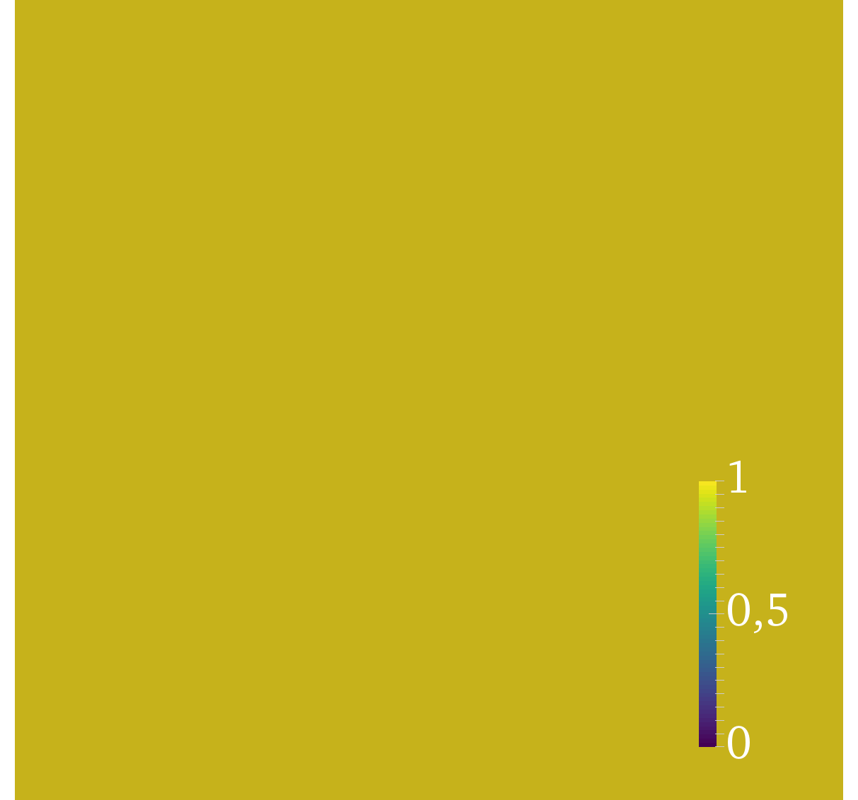
(b) $N_{1,0}$

(c) $N_{2,0}$

(d) $N_{3,0}$

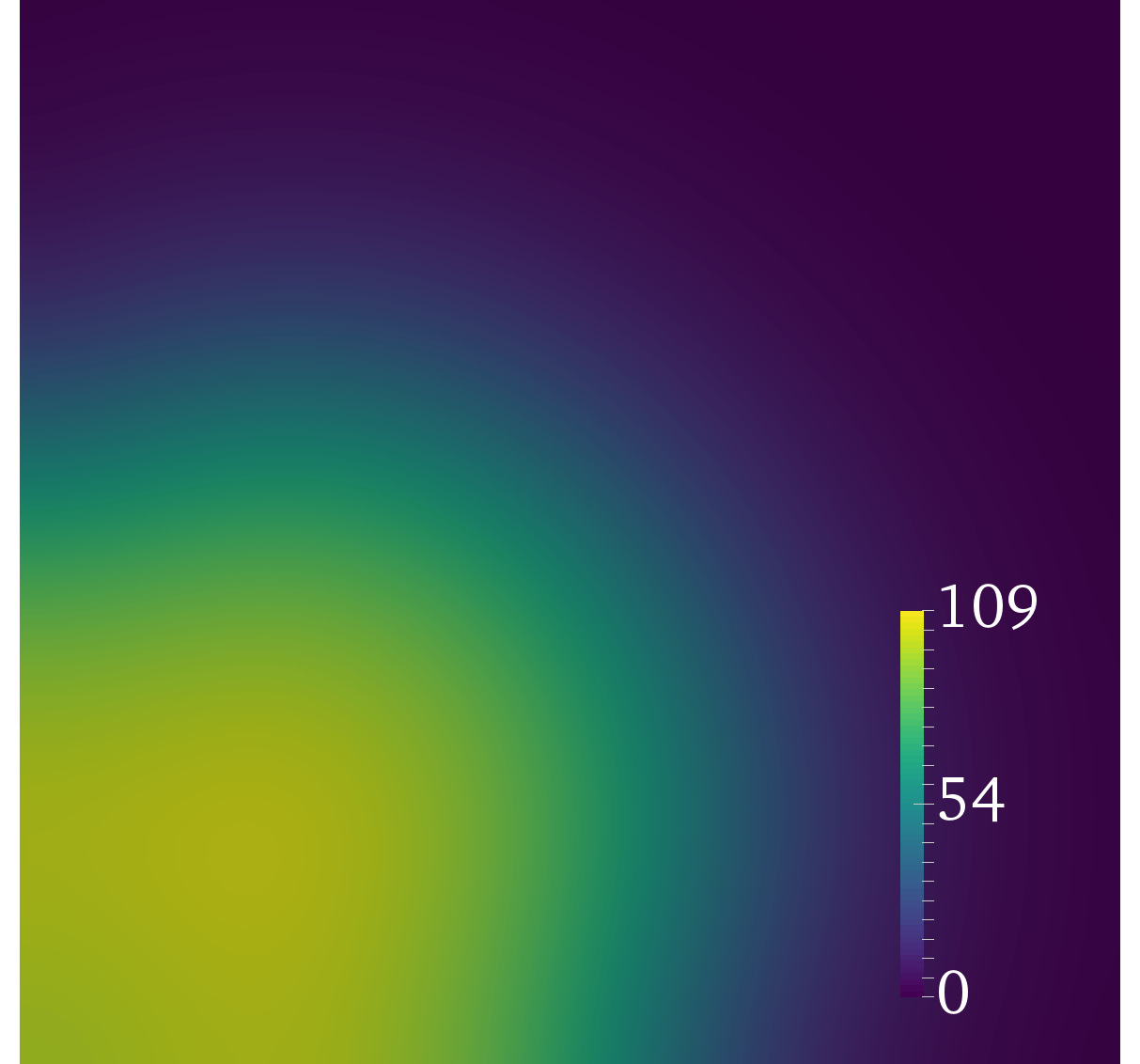
(e) $u(T)$

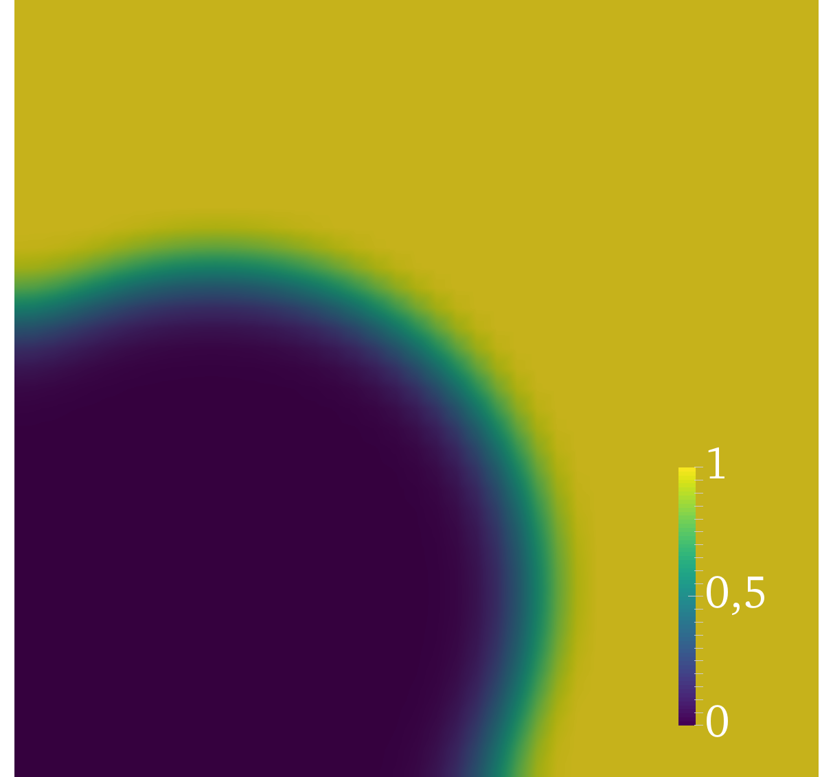
(f) $N_{1}(T)$

(g) $N_{2}(T)$

(h) $N_{3(T)}$

Figure 1: Initial conditions and solutions $t=T=35$ for the mitochondrial swelling example with $N_{x}=40$. The scale is common for A and E and ranges from $0$ (blue) to 108.3 (yellow). The scale is common for B-D and F-G and ranges from $0$ (blue) to $1$ (yellow).

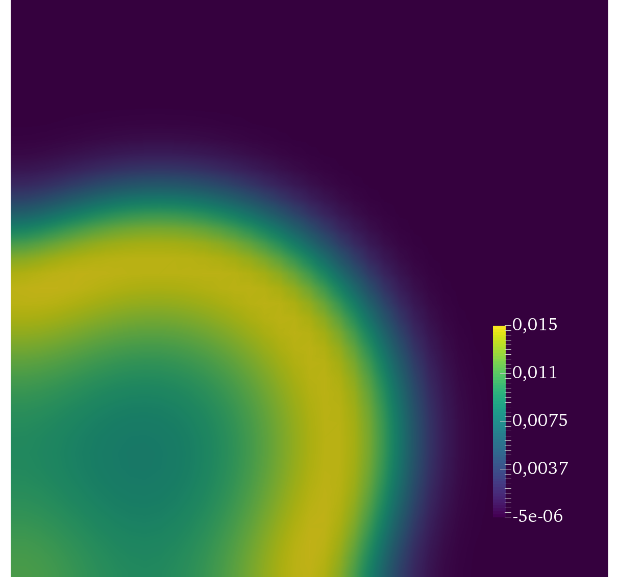
Figure 2: Sensitivity of $J$, the total amount of completely swollen mitochondria at $T$, $L^{2}$-gradient of $J$ (left) with respect to the initial condition $u_{0}$ (right).

To verify that the computed gradient is correct, we performed a Taylor test at a given spatial and temporal resolution with a given perturbation seed. The results are listed in Table 1 and demonstrate the expected orders of convergence, indicating a correctly computed gradient.

$\delta u_{0}$	$R_{0}(\delta u_{0})$	order	$R_{1}(\delta u_{0})$	order
0.5	$1.22\times 10^{-3}$		$1.25\times 10^{-6}$
0.25	$6.14\times 10^{-4}$	1.00	$3.11\times 10^{-7}$	2.00
0.125	$3.07\times 10^{-4}$	1.00	$7.77\times 10^{-8}$	2.00
0.0625	$1.53\times 10^{-4}$	1.00	$1.94\times 10^{-8}$	2.00
0.03125	$7.67\times 10^{-5}$	1.00	$4.85\times 10^{-9}$	2.00

Table 1: Taylor reminders $R_{0}=|J(u_{0}+\delta u_{0})|$ and $R_{1}=|J(u_{0}+\delta u_{0})-J(u_{0})-\nabla J(u_{0})\delta u_{0}|$ for the mitochondria example with functional given by (28) (to three significant digits). Computations performed with $T=35$, $\kappa_{n}=0.5$ and $N_{x}=40$ and the ESDIRK4 scheme.

In a multi-stage scheme, a number of intermediate stage solutions are computed during the solution process. To avoid excessive memory usage, dolfin-adjoint does not store these stage solutions. Thus, in order to compute the adjoint solution, the stage solutions are recomputed for each time-step. As a consequence, the minimal ratio of adjoint runtime to forward runtime for multistage ODE solves using this strategy is approximately 2. For a linear PDE solve, the optimal ratio of adjoint run time to forward run time, assuming all linear solves take the same amount of time, is $1$. For a nonlinear PDE solve via a Newton iteration, the optimal ratio of adjoint run time to forward run time, assuming all linear solves take the same amount of time, is $1/N$ where N is the number of average Newton iterations in the forward solve. These optimal ratios for linear and nonlinear PDE solves have observed for typical dolfin-adjoint usage [10]. For this example, two Newton iterations were required on average to solve the PDEs to within a tolerance of $10^{-10}$ both for $N_{x}=40$ and $80$, and assembly dominated the PDE solve runtime. Thus for this example with two multistage ODE solves and a nonlinear PDE solve in each timestep, the optimal ratio of adjoint runtime to forward runtime is expected to be in the range $0.5-2$, and closer to the upper bound than the lower bound depending on the distribution of computational cost between the PDEs and ODEs.

Experimentally observed timings for this example are listed in Tables 2–3 for $N_{x}=40,80,160$. From Table 2, we observe that the adjoint-to-forward runtime ratio for the total solve is in the range $1.38-1.95$ and decreasing with increasing problem size. The corresponding gradient-to-forward runtime is in the range $1.44-2.28$, again decreasing with increasing problem size as expected. From Table 3, we observe that adjoint-to-forward runtime ratio for the ODE solves is in the range $2.35-2.41$ for this set of problem sizes, also decreasing with increasing problem size. We also note that the ODE solve runtime, both for the forward and adjoint solves, appears to scale linearly with the problem size $M=N_{x}^{2}$ as anticipated and as is optimal. The ODE solves account for $37-40\%$ of the total forward runtime for this example.

$N_{x}$	Forward $t_{F}$ (s)	Adjoint $t_{A}$ (s)	Ratio $\frac{t_{A}}{t_{F}}$	Gradient $t_{G}$ (s)	Ratio $\frac{t_{G}}{t_{F}}$
$40$	9.30	18.1	1.95	21.2	2.28
$80$	34.0	52.2	1.53	56.1	1.65
$160$	135	186	1.38	193	1.44

Table 2: Run times to compute the forward solution $t_{F}$ and to compute the adjoint $t_{A}$ and the functional gradient $t_{G}$ of the functional defined by (28) for the mitochondria example with increasing spatial resolution for $T=35$ $\kappa_{n}=0.5$ with the ESDIRK4 multistage scheme.

$N_{x}$	Forward ODEs (s)	(of total)	Adjoint ODEs (s)	Ratio
	$t_{F,O}$		$t_{A,O}$	$\frac{t_{A,O}}{t_{F,O}}$
$40$	3.48	(37 %)	8.40	2.41
$80$	13.7	(40 %)	32.6	2.37
$160$	53.6	(40 %)	126	2.35

Table 3: Run times for solving the ODE systems when computing the forward solution $t_{F,O}$ and when computing the adjoint $t_{A,O}$ of the functional defined by (28) for $T=35$ $\kappa_{n}=0.5$ with the ESDIRK4 multistage scheme.

We also conducted numerical experiments varying the multistage scheme used in the ODE solves, including the 1-stage Backward Euler (BDF1), the 2-stage Crank-Nicolson (CN2), the 3-stage ESDIRK3 scheme in addition to the previously reported 4-stage ESDIRK4 scheme. The results (using $N_{x}=40$) are reported in Table 4. We observe that the adjoint-to-forward runtime ratio ranges from $2.04$ (BDF1) to $2.41$ (ESDIRK3, ESDIRK4) and the general trend is that this ratio increases with the number of stages as expected, but stabilizes around $2.3-2.4$.

Scheme	Forward	Forward ODEs (s)	Adjoint ODEs (s)	Ratio
	$t_{F}$	$t_{F,O}$	$t_{A,O}$	$\frac{t_{A,O}}{t_{F,O}}$
BDF1	6.56	0.76	1.55	2.04
CN2	6.67	0.94	2.14	2.28
ESDIRK3	8.30	2.54	6.02	2.37
ESDIRK4	9.30	3.48	8.40	2.41

Table 4: Run times computing the forward solution $t_{F}$, for solving the ODE systems when computing the forward solution $t_{F,O}$ and when computing the adjoint $t_{A,O}$ of the functional defined by (28) for $T=35$ $\kappa_{n}=0.5$, $N_{x}=40$ for some common multistage schemes.

6.2 Application: cardiac electrophysiology (2D)

In this example, we consider the bidomain equations (2) over a two-dimensional rectangular domain $\Omega=[0,50]\times[0,50]$ (mm) with coordinates ($x_{0},x_{1}$). We will consider a set of different cardiac cell models of increasing complexity: a reparametrized FitzHugh-Nagumo (FHN) model with 1 ODE state variable [11], the Beeler-Reuter (BR) model with 7 ODE state variables [5], the ten Tusscher and Panfilov (TTP) epicardial cell model with 18 ODE state variables [28], and the Grandi et al (GPB) cell model with 38 ODE state variables [13]. The description of each of these cell models is available via the CellML repository, and our implementation of the ionic current $I_{\rm ion}$ and $F$ arising in (2) was automatically generated from the CellML models for the BR, TTP and GPB models. We refer to the supplementary code [9] for the precise description of the models including our choice of FitzHugh-Nagumo parameters.

Our parameter setup is otherwise as follows. We let $\chi=140$ (mm^-1), $C_{m}=0.01$ ($\mu$F/mm²), and let $M_{i}=\mathrm{diag}(g_{\rm if},g_{\rm if})$ and $M_{e}=\mathrm{diag}(g_{\rm ef},g_{\rm es})$ where $g_{\rm ef}=0.625/(\chi C_{m})$, $g_{\rm es}=0.236/(\chi C_{m})$ and $g_{\rm if}=0.174/(\chi C_{m})$. We let $I_{s}=0$ and set the initial condition

(31) $$v_{0}=10\left(\frac{x_{0}}{50}\right)^{2}+10$$

for $v$. The other state variables are initialized to the default initial conditions given by the respective CellML models.

We use a second-order Strang splitting scheme (i.e. $\theta=0.5$ for (4)–(5)), a Crank-Nicolson discretization in time and continuous piecewise linear finite elements in space for the PDE system, and different Rush-Larsen type discretizations (RL1, GRL1, RL2, GRL2) for the time discretization of the ODE systems. The coupled linear systems that arise at each PDE step (5) were solved with a block-preconditioned GMRES scheme with a relative tolerance of $10^{-10}$. The complete details of the solver are detailed in the supplementary code [9].

We take $\kappa_{n}=0.1$ (ms), and consider a uniform mesh of the computational domain with $N_{x}\times N_{x}\times 2$ triangles. The coarsest mesh considered used $N_{x}=160$. For this case, simulations converged using any of the cell models and schemes, and gave qualitatively correct results, except the Grandi cell model discretized by the RL1 scheme for which the numerical solution scheme failed to converge.

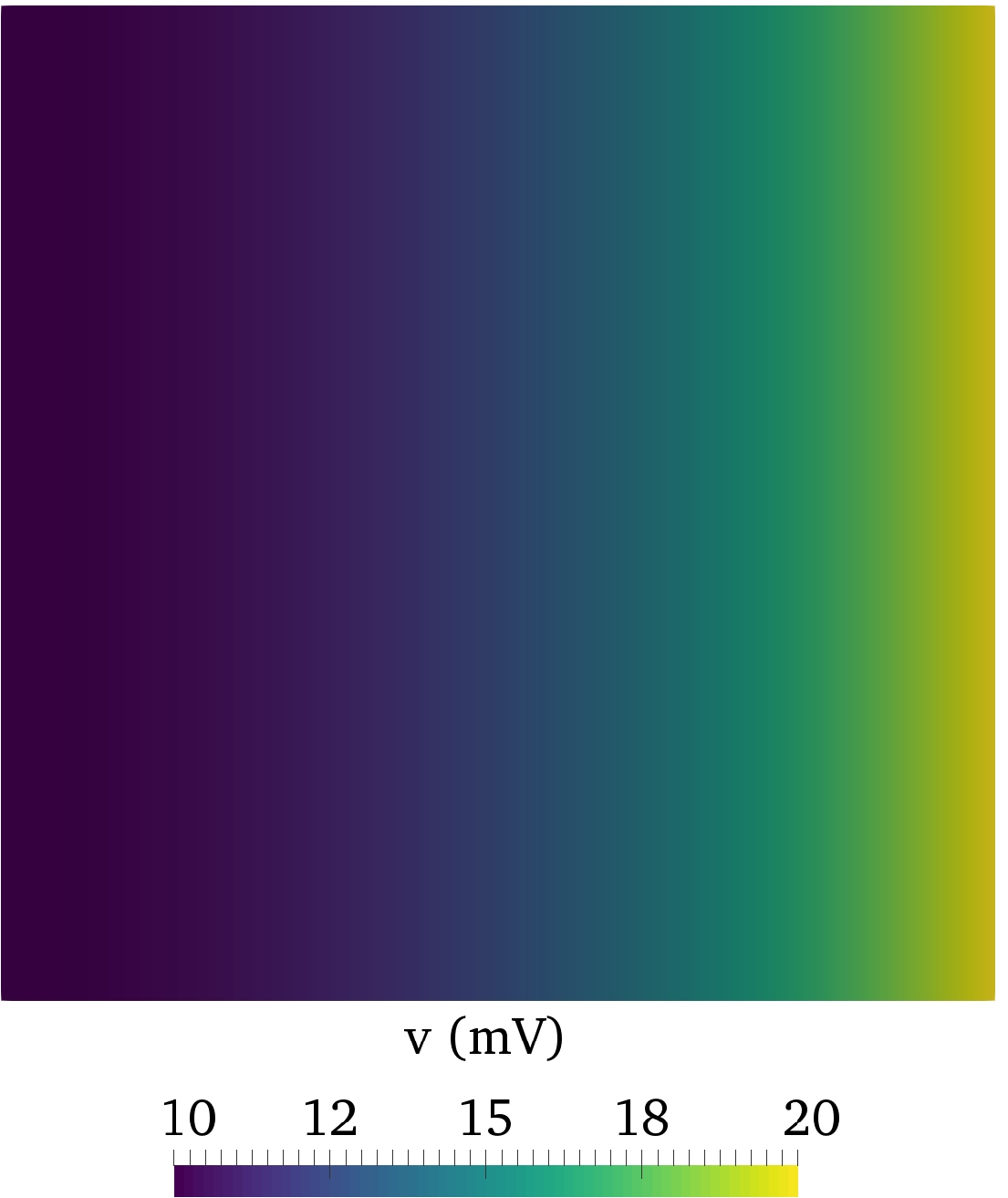
(a) t=0 ms

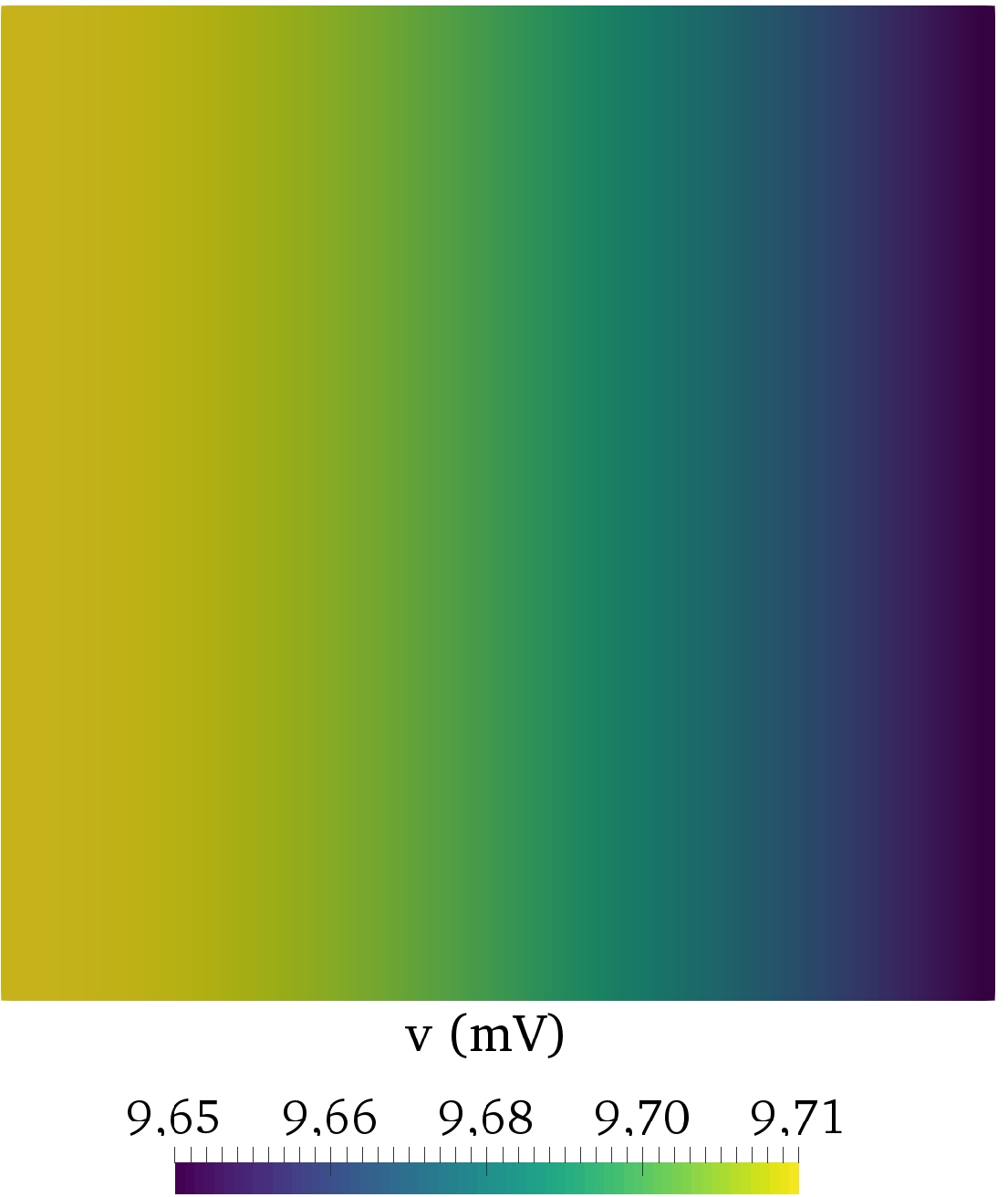
(b) t=100 ms

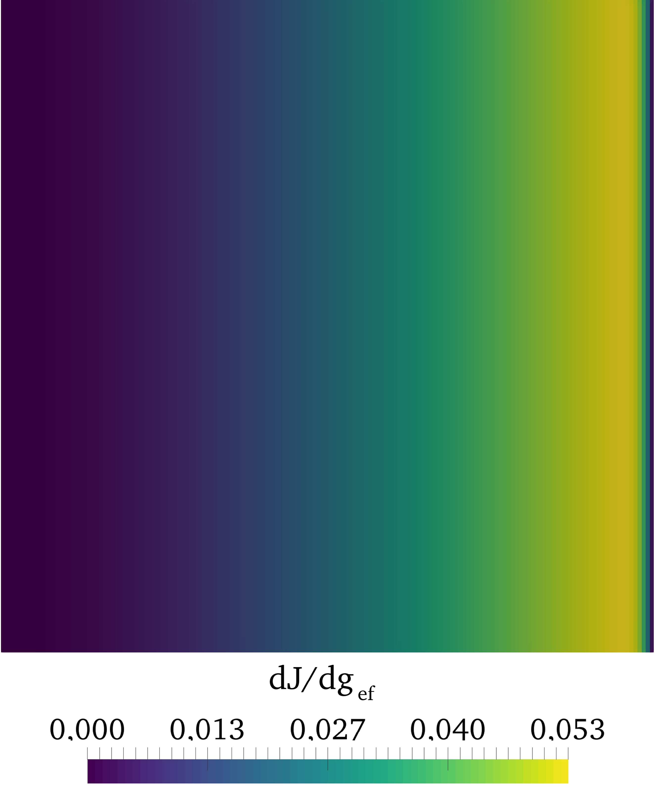
(c) dJ/dg_ef

(d)

Figure 3: (a) Transmembrane potential $v$ at $t=0$ ms and (b) at $t=100$ ms using the FHN model, computed with $\kappa_{n}=0.1$ and $N_{x}=160$. (c) $L^{2}$-gradient of the functional with respect to the extracellular fiber conductivity $g_{ef}$. (d) Timeplot of transmembrane potential $v$ at $x=y=25$ mm.

We are interested in computing the gradient with respect to the extracellular fiber conductivity $g_{\rm ef}$ of the following objective functional

(32) $$J(v)=\sum_{i=1}^{5}\int_{\Omega}\left(v(t_{i})^{2}+s(t_{i})^{2}\right)\,\mathrm{d}x$$

for a equidistributed set of time points $t_{i}$. The model initial condition and solution for the transmembrane potential at $T=100$, together with the $L^{2}$-gradient of the objective functional with respect to the fiber conductivity are illustrated in Figure 3.

The following numerical experiments were performed on the Abel supercomputer at the University of Oslo. All runtime experiments were repeated three times, of which the minimum timing values are reported here.

6.2.1 Verifying the correctness of the discrete gradient

To verify that the computed functional gradient is correct, we performed a Taylor test in a random perturbation direction at given spatial and temporal resolutions. The results with the Fitz-Hugh Nagumo cell model and the GRL1 scheme are listed in Table 5 and demonstrate the expected orders of convergence without a computed gradient (order 1) and when using the computed discrete gradient (order 2) in the Taylor expansion.

$s$	$R_{0}(s)$	order	$R_{1}(s)$	order
0.005	15.7	0.96	0.541
0.0025	7.97	0.98	0.145	1.90
0.00125	4.02	0.99	0.0382	1.92
0.000625	2.02	0.99	0.00983	1.96

Table 5: Taylor convergence results for the cardiac electrophysiology 2D test case. Taylor remainders $R_{0}=|J(g_{ef}+s\delta)|$ and $R_{1}=|J(g_{ef}+s\delta)-J(g_{ef})-\nabla J(g_{ef})s\delta|$ for decreasing step sizes $s$ and a random direction $\delta$ with functional given by (32). Computations performed with $T=10.0$, $\kappa_{n}=0.1$ and $N_{x}=160$, the FHN cell model and the GRL1 scheme. We observe that the remainders converge at first order without gradient information and at second order with gradient information, as expected.

We also performed similar experiments for the other cell models (BR, TTP, and GPB) and other Rush-Larsen solution schemes (RL1, GRL2, RL2). We used the same settings as in Table 5, except for the Grandi cell model with any other Rush-Larsen scheme than GRL1, where the time step had to be reduced to 0.01 in order for the forward solver to converge. We obtained the expected convergence order for all combination of cell models and schemes tested. These results indicate that the automatically derived and computed adjoints and gradient are correct for all the Rush-Larsen schemes implemented.

6.2.2 Adjoint runtime performance

As the bidomain PDEs (5) are linear, a rough theoretical estimate of the optimal PDE adjoint to PDE forward runtime ratio is 1, assuming that the solution times in the adjoint and forward PDE solves are equal and dominated by the finite element assembly and linear solvers. Similarly, the ODEs are solved with explicit Rush-Larsen schemes with a theoretically optimal adjoint-to-forward ratio of 1 as well.

In Table 6, we list the total runtime, and the runtime components corresponding to only the ODE solves, only the PDE solves and an intermediate variable update (merge) step, for both the forward and the adjoint solution computation for a test case with $T=10.0$, $\kappa_{n}=0.1$, $N_{x}=160$, the GRL1 scheme and the four different cardiac cell models (FHN, BR, TTP, GPB).

Model		Total	ODEs	PDEs	Merge	Other
FHN	Forward	38.8	3.20	34.1	0.466	3 %
	Adjoint	44.4	8.27	28.1	1.75	14 %
	Ratio	1.15	2.58	0.82	3.76
BR	Forward	48.3	10.9	34.5	0.979	4 %
	Adjoint	62.1	20.4	28.2	4.66	14 %
	Ratio	1.29	1.88	0.81	4.76
TTP	Forward	67.3	24.4	35.5	1.97	8 %
	Adjoint	99.5	47.8	28.2	9.98	14 %
	Ratio	1.48	1.96	0.79	5.07
GPB	Forward	91.8	40.8	34.7	3.63	14 %
	Adjoint	152	81.7	28.2	19.6	15 %
	Ratio	1.66	2.00	0.81	5.40

Table 6: Adjoint-to-forward runtime performance for a cardiac electrophysiology 2D test case. Breakdown of forward and adjoint runtimes and their ratio for different cell models. Each row shows total runtime (s), runtime for the ODE, PDE and merge steps (s), and percentage of the total runtime not accounted for by these three steps (Other). The computations were performed with $T=10$, $\kappa_{n}=0.1$, $N=160$, GRL1 as the ODE scheme and (32) as the adjoint functional.

From Table 6, for the forward solves, we observe that the total runtime increases with cell model complexity. The forward PDE step runtime is essentially independent of the cell model, while the forward ODE step runtime increases with the cell model complexity, as expected: the ODE runtime corresponds to approximately $10\%$ of the PDE runtime for the simplest FitzHugh-Nagumo model, and approximately $114\%$ of the PDE runtime for the most complex Grandi model. The runtime of the forward merge step is insignificant in comparison to the ODE and PDE steps, but increases with cell model complexity.

We observe that also the adjoint PDE runtimes are comparable for all cell models. The resulting adjoint-to-forward PDE step ratios are in the range $0.79-0.82$. The decrease in compute time for the adjoint PDE solves compared to the forward PDE solves are attributable to the Krylov solvers: fewer Krylov solver iterations were necessary for convergence for the adjoint solves compared to the forward solves. For the ODE solves, we observe that the adjoint-to-forward ratio for the ODE solves is in the range $1.88-2.58$ for the different cell models. Additionally, we observe that the runtime of the adjoint merge step is significantly larger than the corresponding time for the forward merge step and with an increasing adjoint-to-forward ratio with increasing cell model complexity $3.76-5.40$. We suggest that the reason for the increased and increasing adjoint runtime is that the adjoint merge step involves additional assembly of variational forms of complexity comparable to that of the cell model.

Overall, we observe that the adjoint-to-forward total runtime ratios are in the range $1.15-1.66$ for the different cell models considered, with increasing adjoint-to-forward ratio with increasing cell model complexity. Since the PDE runtime dominates the total runtime for the simpler cell models, the total adjoint-to-forward ratio is closer to $1$ for these models. On the other hand, for the more complicated cell models, the ODE runtimes dominate, and so we observe adjoint-to-forward ratios closer to $2$ for these.

In the last column of Table 6, we observe that the combined ODE and PDE solve time contributes to between 97% (for FitzHugh-Nagumo) and 86% (for Grandi) of the total forward runtime for the cell models considered. The remaining forward runtime cost is primarily caused by the initialization routines such as loading the computational mesh, and creating the required function spaces. For the corresponding adjoint runtimes, the combined ODE and PDE solve times contribute to between 86% (for FitzHugh-Nagumo) and 85% (for Grandi) of the total run time, and the percentage contribution decreases with the complexity of the cell model. The remaining runtime cost can primarily be attributed to recording the forward states during the adjoint solve (which is included in the reported total run time but not in the ODE or PDE runtimes here). We also timed the computation of the discrete gradient and noted that the cost of additionally computing the gradient was negligible (less than 0.1% of the adjoint solve runtime).

6.2.3 Forward and adjoint parallel scalability

In this section, we discuss the weak and strong parallel scalability of the forward and adjoint ODE solvers and the scalability of the point integral solvers in particular applied to this 2D electrophysiology test case. We focus on the scalability of the point integral solver particular as this is the primary new feature described in this paper. Previous studies have discussed the parallel scalability of FEniCS in general [24, 1, 10].

We ran a series of weak scaling experiments on Abel, hosted by the Norwegian national computing infrastructure (NOTUR), for the previously considered series of cell models (FHN, BR, TTP, GPB) on an increasing number of CPUs (1, 4, 16, 64) and with an increasing mesh resolution. We timed the total runtime of the point integral solves, both for the forward solves and the adjoint solves. For each cell model and resolution, we ran three experiments and extracted the minimal run times. The results are listed in Table 7. For both the forward and adjoint run times, we computed the parallel efficiency (PE) as the ratio of the 1-CPU runtime to the $n$-CPU run time for $n=4,16,64$, also listed in Table 7. The optimal PE would be 1. The last column of the Table lists the computed the adjoint-to-forward ratio for these solves.

For the forward runtimes, we observe that the parallel efficiencies range from 0.66 to 0.95 for all cell models and resolutions, with efficiencies higher than 0.8 for all but the least complex cell model. In general, we observe that the parallel efficiency increases with increasing cell model complexity and that it decreases moderately with the number of CPUs. Some of the loss of parallel efficiency (from 1) is attributable to only a near-perfect distribution of mesh vertices across CPUs; we observed approximately 10% variation between CPUs in the number of local vertices.

For the adjoint runtimes, we observe parallel efficiencies ranging from 0.75 (FHN on 64 cores) to 0.95, again with efficiencies higher than 0.8 for all but the least complex cell model. In general, we note the same trends as for the forward run times: increasing parallel efficiency with increasing cell model complexity and moderately decreasing parallel efficiency with increasing number of CPUs. We emphasize that we thus achieve the same parallel efficiency for the adjoint point integral solves as for the forward point integral solves.

Comparing the forward and adjoint runtimes, we see that the adjoint-to-forward ratio for the point integral solvers range from 1.19 to 1.56. Comparing these numbers with the adjoint-to-forward ratios of the overall ODE solves as discussed in the previous, we observe that the adjoint-to-forward point integral solver performance is better. The adjoint-to-forward ratio is moderately increasing with cell model complexity, but is stable with respect to the number of CPUs. This latter point again illustrates that the adjoint point integral solvers demonstrate the same parallel efficiency as the forward point integral solves.

	#CPUs	$N_{x}$	Forward PIS (s)	PE	Adjoint PIS (s)	PE	Ratio
FHN	1	160	0.185		0.251		1.36
	4	320	0.253	0.73	0.311	0.81	1.23
	16	640	0.263	0.70	0.330	0.76	1.25
	64	1280	0.281	0.66	0.333	0.75	1.19
BR	1	160	0.740		0.925		1.25
	4	320	0.795	0.93	0.998	0.93	1.26
	16	640	0.868	0.85	1.076	0.86	1.24
	64	1280	0.899	0.82	1.143	0.81	1.27
TTP	1	160	1.657		2.516		1.52
	4	320	1.736	0.95	2.640	0.95	1.52
	16	640	1.886	0.88	2.939	0.86	1.56
	64	1280	1.991	0.83	3.072	0.82	1.54
GPB	1	160	2.618		3.895		1.49
	4	320	2.771	0.94	4.131	0.94	1.49
	16	640	3.059	0.86	4.553	0.86	1.49
	64	1280	3.125	0.84	4.632	0.84	1.48

Table 7: Weak scaling of the point integral solver for a cardiac electrophysiology 2D test case. Forward and adjoint point integral solver runtimes for increasing $N_{x}$ and simultaneously increasing number of cores and for different cell models. Each row shows number of CPUs, the mesh resolution, the total point integral solver runtime (s) for the forward solves, the parallel efficiency (PE) for the point integral forward solves, the total point integral solver runtime (s) for the adjoint solves, the parallel efficiency for the point integral adjoint solves, and the adjoint-to-forward runtime ratio. The computations were performed with $T=1.0$, $\kappa_{n}=0.1$ and GRL1 as the ODE scheme and (32) as the adjoint functional.

We also ran a series of strong scaling experiments on Abel for the previously considered series of cell models (FHN, BR, TTP, GPB) on an increasing number of CPUs (1, 4, 16, 64) and with a fixed mesh resolution. We timed the total runtime of the point integral solver steps for both the forward and adjoint solves. Again, for each cell model and resolution, we ran three experiments and extracted the minimal run times. The results are listed in Table 8. For both the forward and adjoint run times, we computed the (strong scaling) parallel efficiency (PE) as the ratio of the 1-CPU runtime to $n$-times the $n$-CPU runtime for $n=4,16,64$, also listed in Table 8. The optimal (strong scaling) PE would be 1. The last column of the Table lists the computed the adjoint-to-forward ratio for these solves.

We observe that the parallel efficiencies are comparable to the results from the weak scaling test case with efficiencies in the range from 0.60 to 0.94. We note that the adjoint strong parallel efficiency is comparable to the forward strong parallel efficiency. The adjoint-to-forward ratios for this strong scaling test are also in the same range as for the weak scaling test.

Model	No. cores	Forward PIS	PE	Adjoint PIS	PE	Ratio
FHN	$1$	12.874		17.039		1.32
	$4$	3.503	0.92	4.826	0.88	1.38
	$16$	1.159	0.69	1.373	0.78	1.18
	$64$	0.281	0.72	0.333	0.80	1.19
BR	$1$	48.286		59.673		1.24
	$4$	13.760	0.88	16.455	0.91	1.20
	$16$	3.525	0.86	4.307	0.87	1.22
	$64$	0.899	0.84	1.143	0.82	1.27
TTP	$1$	105.451		161.443		1.53
	$4$	28.003	0.94	44.613	0.90	1.59
	$16$	8.323	0.79	11.451	0.88	1.38
	$64$	1.991	0.83	3.072	0.82	1.54
GPB	$1$	166.582		249.980		1.50
	$4$	45.811	0.91	68.084	0.92	1.49
	$16$	17.426	0.60	25.787	0.61	1.48
	$64$	3.125	0.83	4.632	0.84	1.48

Table 8: Strong scaling of the point integral solver for a cardiac electrophysiology 2D test case. Forward and adjoint point integral solver runtimes for a fixed (fine) mesh resolution $N_{x}=1280$ with an increasing number of CPUs, for different cell models (FHN, BR, TTP, GPB). Each row show the number of CPUs, the total point integral solver runtime for the forward solves, the corresponding parallel efficiency (PE), the total point integral solver runtime for the adjoint solves, the corresponding parallel efficiency (PE) and the adjoint-to-forward runtime ratio. The computations were performed with $T=1.0$, $\kappa_{n}=0.1$ and GRL1 as the ODE scheme and (32) as the adjoint functional.

6.3 Application: biventricular cardiac electrophysiology (3D)

In this example, we aim to compute the sensitivity of the squared $L^{2}$-norm of the transmembrane potential with respect to its initial condition, in order to illustrate the features discussed in this paper for a more complex test case. This example also aims to illustrate how different representations may seamlessly be used for the control variables; this is useful for instance when computing sensitivities with respect to spatially constant, regionally defined or highly resolved control variables.

Inspired by [4], we consider the monodomain variation of (2) over a mesh of a three-dimensional bi-ventricular domain $\Omega$ with the ten Tusscher and Panfilov epicardial cell model [28] as detailed in Section 6.2. For the monodomain equations, we replace the bidomain equations (2a)–(2b) by: find $v$ such that

(33) $$v_{t}-\operatorname{div}M\operatorname{grad}v=-I_{\rm ion}(v,s)\quad\text{ in }\Omega.$$

with homogeneous Neumann boundary conditions and with $v(t=0)=v_{0}$. As before, we let $\chi=140$ (mm^-1), $C_{m}=0.01$ ($\mu$F/mm²), and for simplicity (ignoring realistic, spatially-varying fiber directions), let $M=\mathrm{diag}(g_{\rm f},g_{\rm s},g_{\rm n})$ where:

(34) $$g_{f}=0.255,\quad g_{n}=0.0775,\quad g_{s}=0.0775.$$

To solve the coupled equations (33) and (4), we use a second-order Strang splitting scheme ($\theta=0.5$), a Crank-Nicolson discretization in time and continuous piecewise linear finite elements in space for the resulting PDEs, and the first-order generalized Rush-Larsen (GRL1) scheme for the resulting ODEs. We take $\kappa_{n}=0.05$ (ms). The moderately coarse mesh has mesh cell diameters in the range $[0.61,2.70]$ (mm) and bounding box $[0.103,40.2]\times[-15.8,36.8]\times[-30,13.9]$ (mm³), with 45 625 vertices and 236 816 cells, and is illustrated in Figure 4.

To quantify the transmembrane potential exceeding a zero threshold , we consider the following objective functional:

(35) $$J(v)=\int_{\Omega_{v}}v(T)^{2}\,\mathrm{d}x,$$

at a fixed time $T=6.0$ (ms) and where $\Omega_{v}=\{x\in\Omega\,|\,v(x)\geq 0\}$. We are interested in computing the gradient of $J$ with respect to the initial condition $u_{0}$.

We consider two different representations of the initial condition to illustrate computing the gradient with respect to low and high resolution fields. For both cases, we let

(36) $$v_{0}(x)=\begin{cases}-61.1&x_{2}>z_{\rm mid},\\ -61.3&x_{2}\leq z_{\rm mid},\\ \end{cases}$$

with $z_{\rm mid}=-8.07$, but consider (i) $v_{0}$ as represented by two constants $(c_{0},c_{1})$ i.e. the two-dimensional space $\mathbb{R}^{2}$ and (ii) $v_{0}$ represented by a continuous piecewise linear defined relative to the mesh i.e. as a $n_{\rm verts}$-dimensional space $V$ where $n_{\rm verts}$ denotes the number of mesh vertices.

The initial condition and computed solution at $t=6.0$ (ms) are illustrated in Figure 4. (With reference to the chosen perspective in this Figure, we denote the subdomain where $x_{2}>z_{\rm mid}$ as the top part of the domain and the subdomain $x_{2}\leq z_{\rm mid}$ as the bottom part.)

For the case where the initial condition is represented at a low resolution by $v_{0}=(c_{0},c_{1})\in\mathbb{R}^{2}$, we considered a series of experiments starting with different initial conditions $v_{0}^{\alpha}=(c_{0}+\alpha,c_{1}+\alpha)\in\mathbb{R}^{2}$ for $\alpha\in\{-0.1,-0.05,0.0,0.05,0.1\}$. The resulting gradients (in $\mathbb{R}^{2}$) with respect to $v_{0}\in\mathbb{R}^{2}$ are illustrated in Figure 5 (left). We observe that as we increase $\alpha$, the gradient with respect to the top initial condition $c_{0}$ goes from large and positive to small and negative, while the gradient with respect to the bottom initial condition $c_{1}$ varies from moderately negative to close-to-zero and rapidly to large and positive. The rapid changes in the gradients illustrate the nonlinear nature of the problem at hand.

The sensitivity of the objective functional $J$ defined by (35) with respect to the initial condition $v_{0}\in V$ is illustrated in Figure 5 (right). We observe that the gradient in the upper part of the domain is large and negative, that the gradient in a boundary zone is large and positive and the gradient in the lower part of the domain is close to zero. This indicates that infinitesimal increases/decreases in the upper part of the domain will lead to a large decrease/increase in the functional value, infinitesimal increases/decreases in the boundary zone domain will lead to a large increase/decrease in the functional value, and that infinitesimal increases/decreases in the lower part of the domain will have relatively small effect on the functional value.

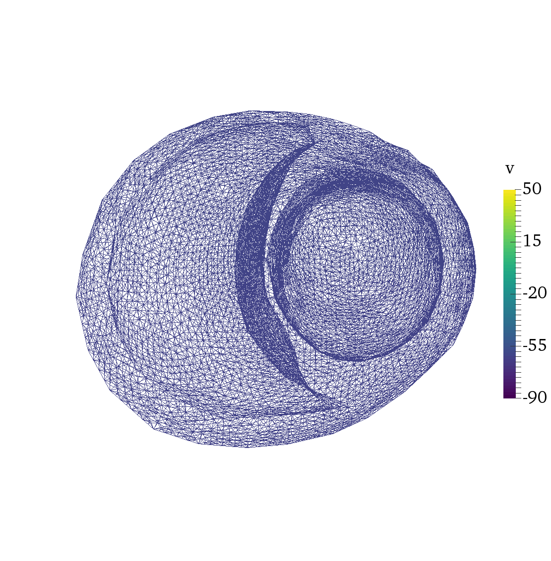
Figure 4: Transmembrane potentials: wireframe view (along positive x-axis) of the computed transmembrane potential $v(t)$ at $t=0$ (left) and $t=6.0$ ms (right).

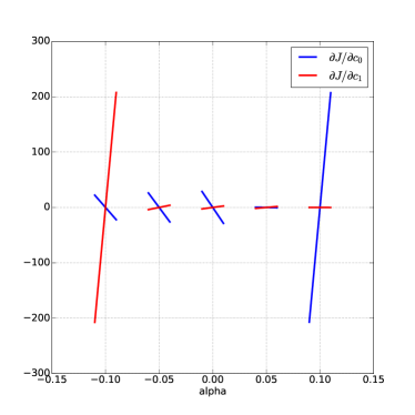
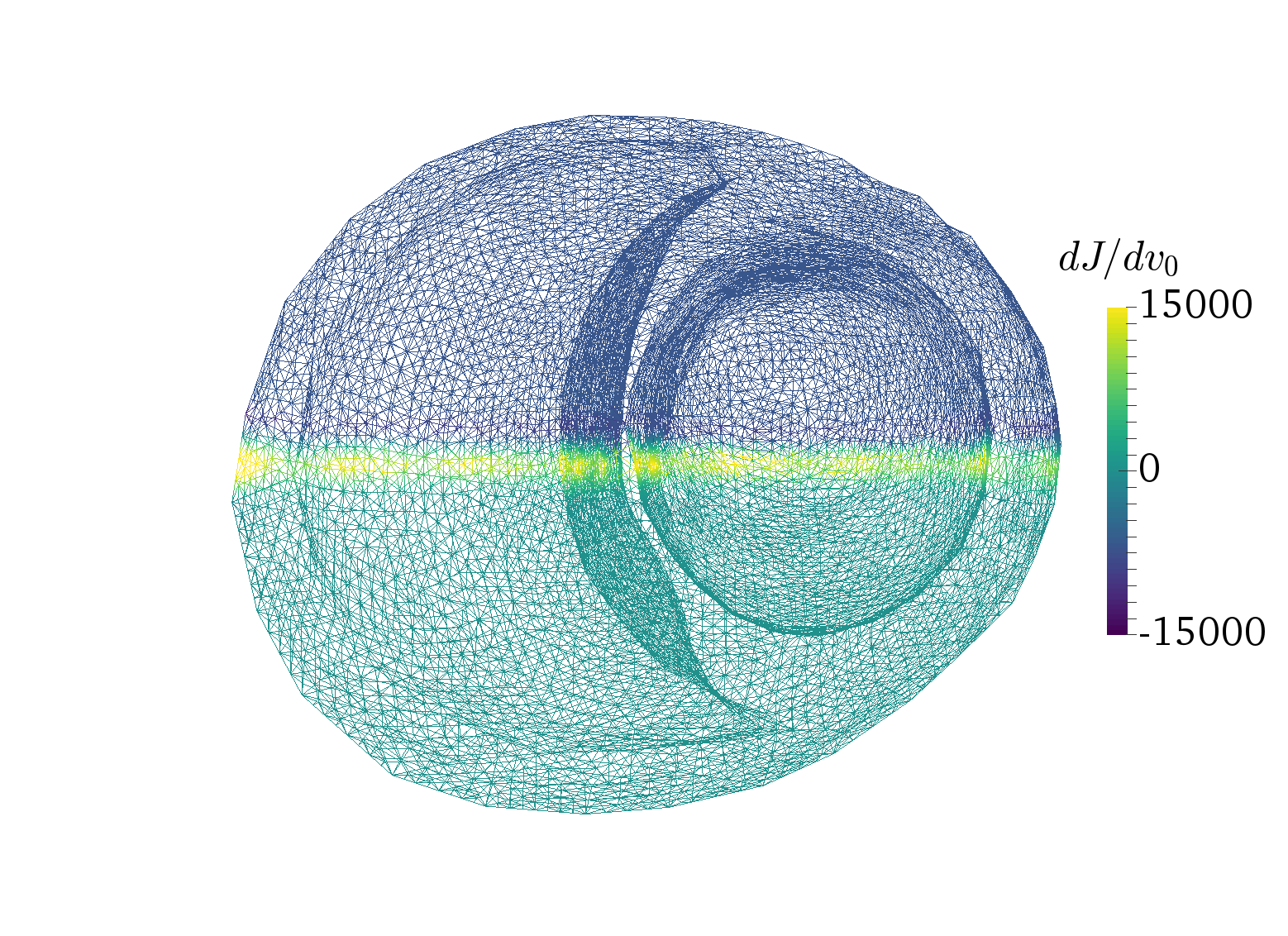
Figure 5: Sensitivities computed with respect to low and high resolution representations of an initial transmembrane potential. Left: sensitivities $\tfrac{\partial J}{\partial v_{0}}=(\tfrac{\partial J}{\partial c_{0}},\tfrac{\partial J}{\partial c_{1}})$ of the objective functional $J$ defined by (35) with respect to a low resolution initial condition $v_{0}=(c_{0},c_{1})\in\mathbb{R}^{2}$ for different initial conditions $v_{0}=v_{0}^{\alpha}=(-61.1+\alpha,-63.3+\alpha)$ for $\alpha=\{-0.1,-0.05,0.0,0.05,0.1\}$. For each point $\alpha$ and $i=0,1$, each plotted line segment (spanning from $\alpha-0.01$ to $\alpha+0.01$) has slope $\tfrac{\partial J}{\partial c_{i}}$. Right: Sensitivity $\tfrac{\partial J}{\partial v_{0}}$ of the objective functional $J$ defined by (35) with respect to high resolution initial condition $v_{0}\in V$.

7 Concluding remarks

We have presented a high-level framework that allows for the specification of coupled PDE-ODE systems and their efficient forward and adjoint solution with operator splitting schemes. We have illustrated the features of the framework with a series of examples originating from cell modelling and computational cardiac electrophysiology. Our numerical results indicate adjoint runtime performance near optimal (measured in terms of adjoint-to-forward runtimes), and parallel efficiency indices of $84-94\%$ for the more realistic cardiac cell models.

The main advantages of the framework are the speed of developing solvers for new systems, and the ability to automatically derive their adjoints from the high-level specification. This allows for flexible exploration of models when the relevant governing equations are uncertain, and for the identification of unknown parameters via the solution of inverse problems as demonstrated e.g. in [14]. Both of these capabilities are of significant importance in numerous areas of scientific computing, and in particular in computational medicine, physiology and biology. Future work will focus on further improving the parallel scalability of the solvers and its application to problems in personalized medicine.

References

- [1] M. S. Alnæs, J. Blechta, J. Hake, A. Johansson, B. Kehlet, A. Logg, C. Richardson, J. Ring, M. E. Rognes, and G. N. Wells, The fenics project version 1.5, Archive of Numerical Software, 3 (2015), https://doi.org/10.11588/ans.2015.100.20553.
- [2] M. S. Alnæs, A. Logg, K.-A. Mardal, O. Skavhaug, and H. P. Langtangen, Unified framework for finite element assembly, International Journal of Computational Science and Engineering, 4 (2009), pp. 231–244, https://doi.org/10.1504/IJCSE.2009.029160.
- [3] M. S. Alnæs, A. Logg, K. B. Ølgaard, M. E. Rognes, and G. N. Wells, Unified form language: A domain-specific language for weak formulations of partial differential equations, ACM Transactions on Mathematical Software, 40 (2014), https://doi.org/10.1145/2566630.
- [4] H. J. Arevalo, F. Vadakkumpadan, E. Guallar, A. Jebb, P. Malamas, K. C. Wu, and N. A. Trayanova, Arrhythmia risk stratification of patients after myocardial infarction using personalized heart models, Nature communications, 7 (2016).
- [5] G. W. Beeler and H. Reuter, Reconstruction of the action potential of ventricular myocardial fibres, The Journal of physiology, 268 (1977), pp. 177–210.
- [6] G. J. Bignell and P. R. Johnston, Split operator finite element method for modelling pulmonary gas exchange, in Proceedings of the 13th Biennial Computational Techniques and Applications Conference, CTAC-2006, W. Read and A. J. Roberts, eds., vol. 48 of ANZIAM J., Aug. 2007, pp. C364–C380. http://anziamj.austms.org.au/ojs/index.php/ANZIAMJ/article/view/125 [August 9, 2007].
- [7] J. C. Butcher, Numerical methods for ordinary differential equations, John Wiley & Sons, 2008.
- [8] S. Eisenhofer, A coupled system of ordinary and partial differential equations modeling the swelling of mitochondria, PhD thesis, Technical University of Munich, 2013.
- [9] P. E. Farrell, J. E. Hake, S. W. Funke, and M. E. Rognes, Supplementary code for ”Automated adjoints of coupled PDE-ODE systems”, Aug. 2017, https://doi.org/10.5281/zenodo.843495, https://doi.org/10.5281/zenodo.843495.
- [10] P. E. Farrell, D. A. Ham, S. W. Funke, and M. E. Rognes, Automated derivation of the adjoint of high-level transient finite element programs, SIAM Journal on Scientific Computing, 35 (2013), pp. C369–C393, https://doi.org/10.1137/120873558.
- [11] R. FitzHugh, Impulses and physiological states in theoretical models of nerve membrane, Biophysical journal, 1 (1961), pp. 445–466.
- [12] J. Geiser, Iterative operator splitting method for coupled problems: Transport and electric fields, Journal of Informatics and Mathematical Sciences, 3 (2011), pp. 107–125.
- [13] E. Grandi, F. S. Pasqualini, and D. M. Bers, A novel computational model of the human ventricular action potential and ca transient, Journal of molecular and cellular cardiology, 48 (2010), pp. 112–121.
- [14] S. Kallhovd, M. M. Maleckar, and M. E. Rognes, Inverse estimation of cardiac activation times via gradient-based optimisation, International Journal for Numerical Methods in Biomedical Engineering, (2017).
- [15] A. Kværnø, Singly diagonally implicit runge–kutta methods with an explicit first stage, BIT Numerical Mathematics, 44 (2004), pp. 489–502.
- [16] A. Logg, K.-A. Mardal, G. N. Wells, et al., Automated Solution of Differential Equations by the Finite Element Method, Springer, 2012, https://doi.org/10.1007/978-3-642-23099-8.
- [17] A. Logg, K. B. Ølgaard, M. E. Rognes, and G. N. Wells, FFC: the FEniCS Form Compiler, Springer, 2012, ch. 11.
- [18] A. Logg and G. N. Wells, Dolfin: Automated finite element computing, ACM Transactions on Mathematical Software, 37 (2010), https://doi.org/10.1145/1731022.1731030.
- [19] G. R. Mirams, C. J. Arthurs, M. O. Bernabeu, R. Bordas, J. Cooper, A. Corrias, Y. Davit, S.-J. Dunn, A. G. Fletcher, D. G. Harvey, et al., Chaste: an open source c++ library for computational physiology and biology, PLoS computational biology, 9 (2013), p. e1002970.
- [20] S. Niederer, L. Mitchell, N. Smith, and G. Plank, Simulating human cardiac electrophysiology on clinical time-scales, Frontiers in physiology, 2 (2011), p. 14, https://doi.org/10.3389/fphys.2011.00014.
- [21] T. O’Hara, L. Virág, A. Varró, and Y. Rudy, Simulation of the undiseased human cardiac ventricular action potential: model formulation and experimental validation, PLoS computational biology, 7 (2011), p. e1002061.
- [22] C. Prud’Homme, V. Chabannes, V. Doyeux, M. Ismail, A. Samake, and G. Pena, Feel++: A Computational Framework for Galerkin Methods and Advanced Numerical Methods, ESAIM: Proceedings, 38 (2012), pp. 429–455, https://doi.org/10.1051/proc/201238024, https://hal.archives-ouvertes.fr/hal-00662868. CEMRACS’11: Multiscale Coupling of Complex Models in Scientific Computing.
- [23] F. Rathgeber, D. A. Ham, L. Mitchell, M. Lange, F. Luporini, A. T. T. McRae, G.-T. Bercea, G. R. Markall, and P. H. J. Kelly, Firedrake: automating the finite element method by composing abstractions, Submitted to ACM TOMS, (2015), http://arxiv.org/abs/1501.01809, https://arxiv.org/abs/1501.01809.
- [24] C. N. Richardson and G. N. Wells, Parallel scaling of DOLFIN on ARCHER. https://doi.org/10.6084/m9.figshare.1304537.v1, Retrieved: 11 35, May 29, 2017 (GMT), 2015, https://doi.org/10.6084/m9.figshare.1304537.v1.
- [25] S. Rush and H. Larsen, A practical algorithm for solving dynamic membrane equations., IEEE Trans Biomed Eng, 25 (1978), pp. 389–392, https://doi.org/10.1109/TBME.1978.326270, http://dx.doi.org/10.1109/TBME.1978.326270.
- [26] J. Sundnes, R. Artebrant, O. Skavhaug, and A. Tveito, A second-order algorithm for solving dynamic cell membrane equations., IEEE Trans Biomed Eng, 56 (2009), pp. 2546–2548, https://doi.org/10.1109/TBME.2009.2014739, http://dx.doi.org/10.1109/TBME.2009.2014739.
- [27] J. Sundnes, G. T. Lines, X. Cai, B. F. Nielsen, K.-A. Mardal, and A. Tveito, Computing the electrical activity in the heart, Springer-Verlag, 2006.
- [28] K. ten Tusscher and A. Panfilov, Cell model for efficient simulation of wave propagation in human ventricular tissue under normal and pathological conditions, Physics in Medicine and Biology, 51 (2006), pp. 6141–6156.
- [29] E. Vigmond, R. W. Dos Santos, A. Prassl, M. Deo, and G. Plank, Solvers for the cardiac bidomain equations, Progress in biophysics and molecular biology, 96 (2008), pp. 3–18.
- [30] F. Wang, J. Bright, and J. Hadfield, Simulating nitrate transport in an alluvial aquifer: a three dimensional n-dynamics model, Journal of hydrology. New Zealand, 42 (2003), pp. 145–162.
- [31] P. J. Whiteley, J. D. Gavaghan, and E. C. Hahn, Mathematical modelling of pulmonary gas transport, Journal of Mathematical Biology, 47, pp. 79–99, https://doi.org/10.1007/s00285-003-0196-8, http://dx.doi.org/10.1007/s00285-003-0196-8.