Surface magnetism in a chiral $d$-wave superconductor with hexagonal symmetry

Abstract

Surface properties are examined in a chiral $d$-wave superconductor with hexagonal symmetry, whose one-body Hamiltonian possesses intrinsic spin-orbit coupling identical to the one characterizing the topological nature of the Kane-Mele honeycomb insulator. In the normal state, spin-orbit coupling gives rise to spontaneous surface spin currents, whereas in the superconducting state, besides the spin currents, there exist also charge surface currents, due to chiral pairing symmetry. Interestingly, the combination of these two currents results in a surface spin polarization, whose spatial dependence is markedly different on the zigzag and armchair surfaces. We discuss various potential candidate materials, such as SrPtAs, which may exhibit these surface properties.

Introduction. Chiral superconductivity is becoming an increasingly hot topic in condensed matter physics. Chiral superconducting states break time-reversal symmetry spontaneously and support chiral surface states, which are of a topological origin. Therefore, they can be viewed as superconducting analogs of the quantum Hall state  Volovik-text . The spin-triplet chiral $p$-wave ($p_{x}\pm ip_{y}$-wave) state is experimentally observed in the $A$ phase of superfluid ³He thin films  Yamashita-etal . It is also the most plausible candidate for pairing symmetry in Sr₂RuO₄  maeno_review_JPSJ_12 . Its realization in the $\nu=5/2$ state of the fractional quantum Hall effect is of great interest due to quasiparticle (vortex) excitations obeying non-abelian statistics.  Read-Green ; 5/2FQHE-exp1 ; 5/2FQHE-exp2 . Another chiral superconducting state is the spin-singlet chiral $d$-wave ($d_{x^{2}-y^{2}}\pm id_{xy}$-wave) state. Although this state has not yet been observed experimentally, there are many potential candidate materials, such as heavily doped graphene  Black-Schaffer-Honerkamp , water-intercalated sodium cobaltates  Kiesel-Platt-Hanke-Thomale , and SrPtAs  Nishikubo-Kudo-Nohara ; Biswas-etal ; Goryo-Fischer-Sigrist ; Fischer-etal ; Fischer-Goryo ; remark . All of these materials exhibit hexagonal symmetry, which results in the degeneracy of $d_{x^{2}-y^{2}}$- and $d_{xy}$-wave pairing components and plays an important role in the stability of the chiral $d$-wave state.

The aim of this paper is to study surface magnetism in chiral $d$-wave superconductors with hexagonal symmetry. In particular, we are interested in the interplay among surface magnetism, surface spin and charge currents, and the topology of the chiral $d$-wave pairing state. To study this, we consider a generic tight-binding model with hexagonal symmetry and spin-orbit coupling compatible with the crystal lattice symmetries. Similar to the Kane-Mele (KM) topological insulator  Kane-Mele , the spin-orbit coupling in this model leads to spontaneous surface spin currents in the normal state. Since these spin currents are carried by states well below the Fermi level, they persist in the superconducting state. To study the surface properties of the superconducting state, we employ a self-consistent Bogoliubov-de Gennes (BdG) approach for slab-shaped systems with zigzag and armchair surfaces. We compute the charge currents  chiral-current ; Kalline ; Tada-Nie-Oshikawa carried by the surface states of the chiral $d$-wave pairing state. Interestingly, we find that the coexistence of spin and charge currents causes a spin polarization spontaneously at the sample surface, similar to the chiral $p$-wave superconductor Sr₂RuO₄  Imai-Wakabayashi-Sigrist . The spatial dependence of the surface spin polarization shows a significant difference in zigzag and armchair surfaces. We note that the superconducting state of the considered hexagonal lattice model belongs to class $D$ of the topological classification  Schnyder-etal , just as the chiral $p$-wave superconductor of Ref.  Imai-Wakabayashi-Sigrist . We expect that our findings are applicable to any class $D$ superconductor with spin-orbit coupling of the KM-model type.

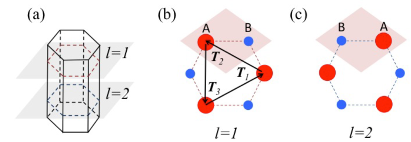
Figure 1: Bilayer honeycomb lattice. (a) Whole unit cell with two distinct honeycomb sublayers. Top view of the two honeycomb sublayers with (b) $l=1$, and (c) $l=2$.

Model definition. Motivated by the hexagonal pnictide superconductor SrPtAs  Nishikubo-Kudo-Nohara , we consider a double-layer hexagonal crystal structure with two honeycomb sublayers depicted in Fig. 1. The two sublattices A and B of each honeycomb layer are taken to be inequivalent, such that each sublayer is noncentrosymmetric (i.e., locally noncentrosymmetric). However, the entire structure has a global inversion center, since the sublattices A and B are exchanged in the two sublayers. To capture the essential physics of such a bilayer honeycomb lattice, we consider for simplicity only the electron hopping on sublattice A (for instance, Pt sites in SrPtAs), while sublattice B only plays the implicit role of breaking local inversion symmetry. The electrons in this system have therefore two internal degrees of freedom: spin and sublayer indices, $\sigma=\uparrow,\downarrow$ and $l=1,2$, respectively. With these assumptions, the tight-binding model for the normal state is described by $H_{0}=H_{t}+H_{c}+H_{c2}+H_{\lambda}$, with

$$H_{t} = t\sum_{n\delta l\sigma}\left(c_{\bm{r}_{n}l\sigma}^{\dagger}c_{\bm{r}_{n}+\bm{T}_{\delta}l\sigma}+c.c.\right)-\mu\sum_{nl\sigma}c_{\bm{r}_{n}l\sigma}^{\dagger}c_{\bm{r}_{n}l\sigma},$$

$$H_{c} = t_{c}\sum_{n\sigma}(c_{\bm{r}_{n}1\sigma}^{\dagger}+c_{\bm{r}_{n}-\bm{c}1\sigma}^{\dagger})\big{(}c_{\bm{r}_{n}2\sigma}+c_{\bm{r}_{n}-\bm{T}_{2}2\sigma}$$

$$\qquad\qquad+c_{\bm{r}_{n}+\bm{T}_{3}2\sigma}\big{)}+c.c.,$$

$$H_{c2} = t_{c2}\sum_{nl\sigma}c_{\bm{r}_{n}l\sigma}^{\dagger}c_{\bm{r}_{n}+\bm{c}l\sigma}+c.c.,$$ (1a)

where $$c_{\bm{r}_{n}l\sigma}^{\dagger} c_{\bm{r}_{n}l\sigma} \bm{r}_{n} n \bm{c} c \bm{T}_{1}=(a,0,0) \bm{T}_{2}=(-a/2,\sqrt{3}a/2,0) \bm{T}_{3}=(-a/2,-\sqrt{3}a/2,0) \mu t t_{c} t_{c2}$$ () stands for the electron creation (annihilation) operator, indicates the position of the th unit cell, is the lattice vector along the axis, and , , and are the three nearest-neighbor in-plane bond vectors. Besides the chemical potential energy , Hamiltonian (1) contains three types of spin-independent hoppings: in-plane , nearest-layer (intersublayer) , and next-nearest-layer (intrasublayer) . In addition, due to the local lack of inversion center in each honeycomb layer, we have the locally antisymmetric spin-orbit coupling

$$H_{\lambda} = i\lambda\sum_{n\delta}\sum_{l\sigma}(-1)^{l}s_{\sigma}c_{\bm{r}_{n}l\sigma}^{\dagger}c_{\bm{r}_{n}+\bm{T}_{\delta}l\sigma}+c.c.,$$ (1b)

where $s_{\uparrow,\downarrow}=\pm 1/2$. Since this term is diagonal with respect to $S_{z}$, Hamiltonian (1) conserves $U(1)_{z}$ symmetry. However, this conservation is only approximate, as it is not protected by the crystalline symmetries. Indeed, there exist spin-dependent next-nearest-layer hopping terms which break $U(1)_{z}$ symmetry  Fischer-Goryo . But these higher-order terms are expected to be small, which is confirmed by band-structure calculations for the case of SrPtAs  Youn-etal . For our numerical calculations we use parameters appropriate for the dominant band of SrPtAs, which consists of two spin-orbit-split Fermi sheets (an open cylindrical one and a closed cigar-shaped one) centered around the Brillouin zone corners  Youn-etal .

In passing we note that Hamiltonian (1) also describes the normal state of UPt₃  Shiozaki-Yanase . Furthermore, we observe that the spin-orbit coupling (1b) is equivalent to the intrinsic spin-orbit coupling of the KM honeycomb quantum spin Hall insulator  Kane-Mele . That is, by identifying the sublayer index in Eq. (1) with the sublattice degree of freedom of the KM model, the latter maps onto Hamiltonian (1) in the limit of letting $t,t_{c2},\mu,c\rightarrow 0$. For this reason, our model (1) describes also the physics of graphenelike structures with large spin-orbit coupling, such as stanene  stanene_nat_mat_15 or graphene on WS₂  WS2_nat_commun .

From the analogy with the KM model  Kane-Mele , it follows that Hamiltonian (1) exhibits a large spin Hall conductivity $\sigma_{xy}^{s}$. Indeed, using the Kubo formula and parameter values appropriate for SrPtAs  Youn-etal , we find that $\sigma_{xy}^{s}\simeq-120\hbar/(e\Omega\textrm{cm})$ [see Appendix A]. This value of $\sigma_{xy}^{s}$ is comparable to that of Pt, which is a typical spin Hall metal  Kimura-etal . We remark that a nonzero $z$ component of spin-orbit coupling is important for a large spin Hall conductivity. A locally noncentrosymmetric system with, for example, only staggered Rashba spin-orbit coupling  Maruyama-etal does not have a net spin Hall conductivity, since the contributions from the two layers cancel out.

To introduce unconventional spin-singlet superconductivity in our model system, we add to Hamiltonian (1) a density-density-type pairing interaction between two electrons on in-plane nearest-neighbor sites in each honeycomb sublayer, i.e.,

$$H_{\textrm{int}}=\frac{U}{2}\sum_{n\delta}\sum_{l\sigma\sigma^{\prime}}n_{\bm{r}_{n}l\sigma}n_{\bm{r}_{n}+\bm{T}_{\delta}l\sigma^{\prime}},$$ (2)

with $U<0$ and $n_{\bm{r}_{n}l\sigma}=c_{\bm{r}_{n}l\sigma}^{\dagger}c_{\bm{r}_{n}l\sigma}$. The attractive pairing interaction (2) is decoupled as usual by BCS-type mean fields with the gap functions $\Delta_{\bm{r}_{n}l}^{(\delta)}=U/2\left<c_{\bm{r}_{n}+\bm{T}_{\delta}l\downarrow}c_{\bm{r}_{n}l\uparrow}-c_{\bm{r}_{n}+\bm{T}_{\delta}l\uparrow}c_{\bm{r}_{n}l\downarrow}\right>,$ which correspond to in-plane spin-singlet pairing in the three different directions ${\bm{T}}_{\delta}$. To determine the order parameters $\Delta_{\bm{r}_{n}l}^{(\delta)}$ we numerically solve the self-consistent gap equation with $U=-0.5$. (We also considered smaller values of $U$, e.g., $U=-0.2$, which leads to qualitatively similar results.) We find that the stable homogeneous solutions of the gap equation satisfy $\Delta^{(1)}=\omega^{2}\Delta^{(2)}=\omega\Delta^{(3)}=\Delta$, where $\omega=e^{i2\pi/3}$. This corresponds to chiral $d$-wave pairing, since the state has eigenvalue $e^{4\pi i}$ with respect to $2\pi$ rotations about the $z$ crystal axis. This chiral $d$-wave state has a nontrivial topology, which is characterized by a quantized Chern number defined in terms of an integral along a two-dimensional submanifold of the three-dimensional Brillouin zone. Choosing, for example, $k_{z}=0$ as the integration plane, the Chern number evaluates to four  Fischer-etal . By the bulk-boundary correspondence, this indicates that four chiral surface states appear at boundaries that are parallel to the (001) direction (see Fig. 6).

Surface properties of the normal state. Before studying the surface properties of the superconducting state, let us first analyze the surface spectrum of the normal state (i.e., $U=0$) at zero temperature. For that purpose, we numerically diagonalize the normal state Hamiltonian (1) in a slab geometry of dimensions $M\times N\times N_{z}=100\times 100\times 100$ with zigzag and armchair surfaces. The zigzag (armchair) surfaces are implemented by imposing periodic boundary conditions in the $z$ direction and the $\bm{T}^{\prime}_{1}$ direction, while imposing open boundary conditions along the $\bm{T}^{\prime}_{2}$ direction [the definitions of $\bm{T}^{\prime}_{1}$ and $\bm{T}^{\prime}_{2}$, and the Fourier transform of the Hamiltonian (1) can be found in Appendix B]. We note that for this slab geometry there are $2N=200$ bands for each spin sector. In Fig. 2 we present the band structure for the up spin sector at $k_{z}=0$. We clearly see in the zigzag case that the $N$ and $(N+1)$th energy bands show a level crossing at $k_{1}=\pi$, which is the trace of the helical edge mode of the KM model. We find that the $N$th band carries a chiral flow of up spin electrons at the front surface, while the $(N+1)$th band carries the counterflow at the back surface. Although it is less clear in Fig. 2, we also have a level crossing hidden inside the bulk bands in the armchair case.

In order to quantify the surface spin current, we compute the thermal expectation value of the spin dependent velocity operator $\langle v_{jl\sigma}\rangle$ at the $j$th site ($j=1,2,...,N$) in the $l$th layer. Using Eq. (1), we find

$$\langle v_{jl\sigma}\rangle=\frac{1}{MN_{z}}\sum_{\bm{k}j^{\prime}l^{\prime}}\left\langle c_{\bm{k}jl\sigma}^{\dagger}\left(\frac{\partial\hat{h}_{0\bm{k}\sigma}}{\partial k_{1}}\right)_{jl;j^{\prime}l^{\prime}}c_{\bm{k}j^{\prime}l^{\prime}\sigma}\right\rangle,$$ (3)

where $\hat{h}_{0\bm{k}\sigma}$ with $\bm{k}=(k_{1},k_{z})$ is the $2N\times 2N$ one-body Hamiltonian matrix with spin $\sigma$. With this, the charge and spin currents are defined as $\langle J_{j}^{c}\rangle=-e\sum_{l\sigma}\langle v_{jl\sigma}\rangle$ and $\langle J_{j}^{s}\rangle=\sum_{l\sigma}s_{\sigma}\langle v_{jl\sigma}\rangle$. Figure 3 shows the spatial distribution of $\langle J_{j}^{s}\rangle$. (Due to time-reversal symmetry there is no charge current in the normal state.) We also plot in Fig. 3 the $\lambda$ and $t_{c}$ dependence of the spin current and find that a nonzero value of both is crucial for a finite spin current. In fact, $J_{\rm sum}^{s}$ is to leading order proportional to $\lambda$ and $t_{c}^{2}$ [Figs. 3(c) and 3(d)], which is in agreement with the analytical expression of $\sigma_{xy}^{s}$ [see Eq. (A5) in Appendix A].

Analogous to the model of Sr₂RuO₄  Imai-Wakabayashi-Sigrist , the origin of this surface spin current can be understood as follows. We see from Fig. 4(a) that an electron with spin $\sigma$ acquires a phase $\phi_{\sigma}=\tan^{-1}s_{\sigma}\lambda/t$ when it travels in the anticlockwise direction along a triangle enclosed by two interplane nearest-neighbor bonds (edges of the hexagon) and an in-plane nearest-neighbor one (dotted line). This results in a circular spin current along the triangle. In the whole system, the spin currents on the inter-plane bonds cancel out in the bulk, but survive at the sample surface. The currents on the in-plane bonds (black arrows in Fig. 4), on the other hand, are not canceled out even in the entire bulk. However, their circulation direction, depicted by colored triangles in Fig. 4, shows a staggered pattern in each sublayer, and hence they are smeared out in the long-wavelength limit. This is anticipated since our model corresponds to the metallic phase of the KM model, which is the spin analog of the Haldane model for the quantum Hall effect without net magnetic flux. Using the above considerations, we can define in the long-wavelength limit a spin-dependent current density  Imai-Wakabayashi-Sigrist $\bm{j}_{\sigma}(\bm{r})=\bm{\nabla}\times\hat{\bm{z}}\Phi_{\sigma}(\bm{r})$, where $\Phi_{\sigma}(\bm{r})=-\Phi_{-\sigma}(\bm{r})$ is the “spin-dependent” flux associated with $\phi_{\sigma}$. It follows that there exists a finite spin current density $\bm{j}_{\uparrow}-\bm{j}_{\downarrow}$ whenever $\Phi_{\sigma}(\bm{r})$ is not uniform, which is the case at the surface.

From Fig. 5 we can see that the surface spin current is carried by Bloch bands well below the Fermi level. The surface current therefore persists in the superconducting phase, since superconductivity does not affect states far from the Fermi level. For the zigzag surface, there is a sharp peak at the $N$th energy band corresponding to a counterpart of the helical edge states.

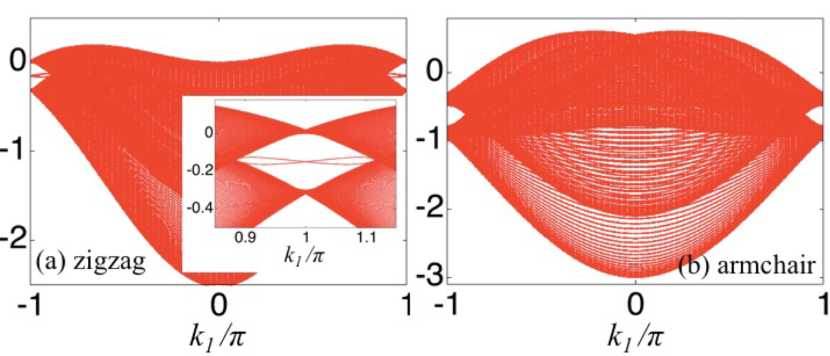
Figure 2: Normal state spectrum at $k_{z}=0$ for (a) the zigzag and (b) the armchair slab. We clearly see the helical edge spectrum in the zigzag case.

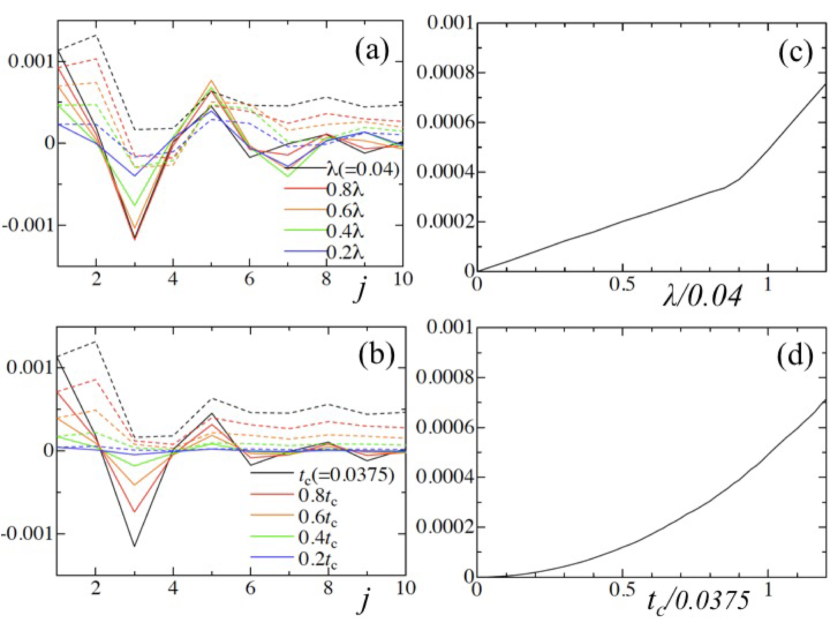
Figure 3: Spatial dependence of the spin current $\langle J^{s}_{j}\rangle$ at the zigzag surface in units of $ta/2$ for several values of (a) spin-orbit coupling $\lambda$ and (b) nearest-inter-sublayer hopping $t_{c}$ with $T=U=0$. Dotted lines are integrated values of the solid lines from $j=0$. Panels (c) and (d) show the $\lambda$- and $t_{c}$-dependence of $J^{s}_{\rm sum}\equiv\sum_{j=1}^{N/2}\langle J^{s}_{j}\rangle$. $\lambda=0.04$ and $t_{c}=0.0375$ are the suggested values for the dominant band in SrPtAs  Youn-etal . For the armchair surface the results are qualitatively similar.

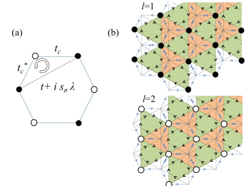
Figure 4: Panel (a) shows the elemental loop for acquiring the spin-dependent phase $\phi_{\sigma}$. The black dots (open circles) on the corners of the hexagon indicate the electron hopping sites in the $l=1$ ($l=2$) sublayer. The arrows in panel (b) show the spin current distribution for the case $\phi_{\uparrow}=-\phi_{\downarrow}>0$, and the colors of triangles show the circulation direction of the spin currents on the intrasublayer bonds (green: clockwise; orange: anti-clockwise).

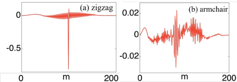
Figure 5: Contribution to the surface spin current $\langle J^{s}_{j=1}\rangle$ in units of $ta/2$ from the $m$th Bloch state at $T=U=0$ for (a) the zigzag and (b) the armchair surface.

Surface properties of the superconducting state. Next, we study the surface properties of the superconducting state. For that purpose, we numerically solve the self-consistent BdG equations for a slab geometry with zigzag and armchair surfaces. We find that the chiral $d$-wave state is a stable solution also in slab geometries. Since the BdG Hamiltonian possesses a mirror symmetry which lets $k_{z}\to-k_{z}$ and exchanges the two sublayers, each eigenstate at $k_{z}=0$ can be labeled by a mirror eigenvalue. This mirror symmetry has two eigensectors at $k_{z}=0$ with two chiral surface states in each eigensector (Fig. 6). We find that the two mirror eigensectors of the BdG Hamiltonian transform into each other under particle-hole symmetry, since the gap function is even under the mirror reflection $k_{z}\rightarrow-k_{z}$  Sato-Ando . That is, while the entire Hamiltonian is particle-hole symmetric, each mirror eigensector breaks this symmetry. Therefore, the energy spectra of the two mirror eigensectors may split. Indeed, this is observed in Fig. 6, which shows the energy spectra at $k_{z}=0$. For the armchair surface the splitting is large enough to see four chiral edge states; for the zigzag surface the splitting is also nonzero, but too small to be seen in Fig. 6(a).

Figure 6: Surface spectrum at $k_{z}=0$ of the chiral $d$-wave superconductor for (a) the zigzag and (b) the armchair slab.

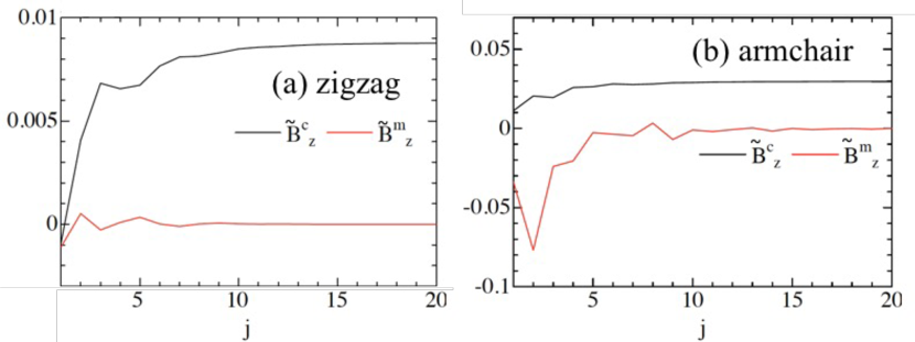
Figure 7: Dimensionless magnetic fields at (a) the zigzag and (b) the armchair surface of the chiral $d$-wave superconductor at $T=0$. The black lines represent the magnetic field $\tilde{B}_{zj}^{c}$ induced by the chiral surface current, while the red lines represent the magnetic field $\tilde{B}_{zj}^{m}$ produced by the spin polarization. Note that the Meissner effect is neglected.

The chiral surface states of Fig. 6 carry a charge current  chiral-current . In addition, the superconducting state exhibits a surface spin current due to states well below the Fermi level, which are not affected by superconductivity. The coexistence of spin and charge currents leads to a spin polarization at the sample surface. Both the charge current and the spin polarization produce net magnetic fields, which are given by  Imai-Wakabayashi-Sigrist

$$B_{zj}^{c} = \mu_{0}\sum_{j^{\prime}}^{j}\langle J^{c}_{j^{\prime}}\rangle=\frac{e\mu_{0}ta}{\hbar S_{0}}\tilde{B}_{zj}^{c},$$ (4a)

$$B_{zj}^{m} = -\frac{\mu_{0}}{\Omega_{c}}\sum_{l\sigma}g\mu_{B}s_{\sigma}n_{j\sigma}=\frac{\mu_{0}\mu_{B}}{\Omega_{c}}\tilde{B}_{zj}^{m},$$ (4b)

where $n_{j\sigma}=\sum_{\bm{k}l}\langle c_{\bm{k}jl\sigma}^{\dagger}c_{\bm{k}jl\sigma}\rangle/(MN_{z})$, $\mu_{0}$ is the magnetic permeability, and $\tilde{B}_{zj}^{c}$ and $\tilde{B}_{zj}^{m}$ are the dimensionless fields on layer $j$. The constants $S_{0}=ac$ and $\Omega_{c}=ka^{2}c$ ($k=1$ for zigzag and $k=\sqrt{3}$ for armchair cases) are the cross section and volume of the unit cell in the slabs, respectively. Note that the Meissner screening is neglected here, which would introduce counter-propagating currents on a length scale of the London penetration depth. In Fig. 7 the two magnetic fields are shown for the zigzag and armchair surfaces. To compare the two fields, the dimensional prefactors $e\mu_{0}ta/\hbar S_{0}$ and $\mu_{0}\mu_{B}/\Omega_{c}$ must be taken into account, which, however, turn out to be of the same order  Imai-Wakabayashi-Sigrist . Hence, we conclude that on the armchair surface the two fields tend to cancel each other, since they have a similar magnitude but opposite sign. This cancellation is independent of the chirality of the $d$-wave state, since the direction of the spin polarization is coupled to the chirality through spin-orbit coupling. On zigzag surfaces, on the other hand, there is no cancellation between the two fields, since $B_{zj}^{m}$ oscillates around zero.

Discussion. We have investigated spin and charge currents at the surfaces of chiral $d$-wave superconductors with hexagonal symmetry and intrinsic spin-orbit coupling. We have shown that the combination of spin and charge currents leads to a spontaneous spin polarization at the surface of the superconductor. Both the spin polarization and the chiral charge currents generate magnetic fields, whose spatial dependence we have studied in detail. These magnetic fields and spontaneous spin polarization could be observed experimentally using scanning Hall probe microscopy, electron spin resonance (ESR), or spin dependent tunneling.

Our results are not only relevant for the hexagonal pnictide superconductor SrPtAs, but also for doped graphenelike structures with strong spin-orbit coupling, such as stanene. Recent muon spin rotation ($\mu$SR) experiments on polycrystalline SrPtAs  Biswas-etal have detected spontaneous magnetic fields in the superconducting state, which is qualitatively in agreement with our findings. Unfortunately, single crystals of SrPtAs are not yet large enough to allow for $\mu$SR measurements  Nohara-private . However, with these small single crystals it might be possible to measure the predicted spin polarization using ESR or spin-dependent tunneling experiments.

The authors thank M. Nohara and M. H. Fischer for their useful discussions. This work was partially supported by JSPS KAKENHI Grant No.15H05885 (J-Physics). J.G. is grateful to the Pauli Center for Theoretical Physics of ETH Zurich for hospitality.

Appendix A The bulk spin Hall conductivity in the normal state

As the system is analogous to the metallic phase of Kane-Mele (KM) model, we would have the spin Hall conductivity. In the Fourier space,

$$H_{0} = \sum_{\bm{k},\sigma}\sum_{l,l^{\prime}}c_{\bm{k}l\sigma}^{\dagger}(\hat{h}_{0\bm{k}\sigma})_{ll^{\prime}}c_{\bm{k}l^{\prime}\sigma},$$

$$\hat{h}_{0\bm{k}\sigma} = \epsilon_{\bm{k}}\hat{\tau}_{0}+\bm{g}_{\bm{k}\sigma}\cdot\hat{\bm{\tau}},$$

$$\bm{g}_{\bm{k}\sigma} = ({\rm Re}(t_{c\bm{k}}),-{\rm Im}(t_{c\bm{k}}),-2s_{\sigma}\lambda_{\bm{k}}),$$

$$\epsilon_{\bm{k}} = -2t\sum_{\delta=1}^{3}\cos\bm{k}\cdot\bm{T}_{\delta}-2t_{c2}\cos k_{z}c-\mu,$$

$$t_{c\bm{k}} = t_{c}(1+e^{i\bm{k}\cdot\bm{T}_{2}}+e^{-i\bm{k}\cdot\bm{T}_{3}})(1+e^{ik_{z}c})=t_{c-\bm{k}}^{*},$$

$$\lambda_{\bm{k}} = \lambda\sum_{\delta=1}^{3}\sin\bm{k}\cdot\bm{T}_{\delta}=-\lambda_{-\bm{k}},$$ (5)

where $\hat{\tau}_{0}$ and $\hat{\bm{\tau}}$ are the $2\times 2$ unit and Pauli matrices with sublayer indices $l$ and $l^{\prime}$. The energy spectrum of $H_{0}$ is $\xi_{\bm{k}}^{\pm}=\epsilon_{\bm{k}}\pm\sqrt{|t_{c\bm{k}}|^{2}+\lambda_{\bm{k}}^{2}}$, and each branch $\pm$ has the Kramers degeneracy. The operators for charge and spin currents are

$$\bm{j} = -e\sum_{\sigma}\bm{v}_{\sigma},$$ (6)

$$\bm{j}_{s} = \sum_{\sigma}s_{\sigma}\bm{v}_{\sigma},$$ (7)

where

$$\bm{v}_{\sigma}=\sum_{ll^{\prime}}\left\{{\bm{\nabla}_{\bm{k}}}\hat{h}_{0\sigma}\right\}_{ll^{\prime}}c_{\bm{k}l\sigma}^{\dagger}c_{\bm{k}l^{\prime}\sigma},$$ (8)

is the spin-dependent velocity operator. We estimate the charge current-spin current correlation function and employ the Kubo formula for the spin Hall conductivity $\sigma_{xy}^{s}$. We neglect the vertex correction and obtain the following form, which reminds us the Skyrmion number

$$\sigma_{xy}^{s} = \frac{e}{2\pi}\int\frac{d^{3}k}{8\pi^{2}}\sum_{\sigma}s_{\sigma}\hat{\bm{g}}_{\bm{k}\sigma}\cdot\left(\partial_{k_{x}}\hat{\bm{g}}_{\bm{k}\sigma}\times\partial_{k_{y}}\hat{\bm{g}}_{\bm{k}\sigma}\right)\times$$ (9)

$$\left(f(\xi_{\bm{k}}^{+})-f(\xi_{\bm{k}}^{-})\right),$$

where $\hat{\bm{g}}_{\bm{k}\sigma}={\bm{g}}_{\bm{k}\sigma}/|{\bm{g}}_{\bm{k}\sigma}|$ and $f(\xi_{\bm{k}}^{\pm})$ is the Fermi distribution function for each subenergy band. Note that $\sigma_{xy}^{s}$ is not quantized even at the zero temperature, because the $k$-integration is over the partially occupied states in the Brillouin zone (not the entire Brilloun zone). Using the tight-binding parameters for all the conduction bands in SrPtAs obtained from the band structure calculation  Youn-etal , we find $\sigma_{xy}^{s}\simeq-120\hbar/(e\Omega{\rm cm})$ at $T=0$. This value is comparable to the spin Hall conductivity of Pt, which is a typical spin Hall metal  Kimura-etal .

Eq. (9) suggests that $\sigma_{xy}^{s}$ is proportional to $\lambda$ and $t_{c}^{2}$ when they are small. We should emphasize here that this behavior is consistent with the results in Fig. 3.

Appendix B Fourier transforms of the non-interacting Hamiltonian (1) in zigzag and armchair slabs

We show the Fourier transforms of the normal state Hamiltonian (1) in zigzag and armchair cases (see Figs. 8 and 9). Let $c_{\bm{k}jl\sigma}^{\dagger}$ ($c_{\bm{k}jl\sigma}$ ) stands for the creation and annihilation operator of the electron at the $j$-th site in the $l$-th layer with momentum $\bm{k}=(k_{1},k_{z})$ and spin $\sigma$, and the results are as follows:

• The zigzag case

  $$H_{t} = 2t\sum_{\bm{k}jl\sigma}\left\{\cos k_{1}c^{\dagger}_{\bm{k}jl\sigma}c_{\bm{k}jl\sigma}+\right.$$

  $$\left.\cos\frac{k_{1}}{2}\left(c^{\dagger}_{\bm{k}jl\sigma}c_{\bm{k}j+1l\sigma}+c.c.\right)\right\},$$

  $$H_{c} = t_{c}\sum_{\bm{k}j\sigma}\left(2\cos\frac{k_{1}}{2}e^{i\frac{k_{z}}{2}}c^{\dagger}_{\bm{k}j1\sigma}c_{\bm{k}j2\sigma}+\right.$$

  $$\left.e^{-i\frac{k_{z}}{2}}c^{\dagger}_{\bm{k}j2\sigma}c_{\bm{k}j1\sigma}+c.c.\right),$$

  $$H_{c2} = 2t_{c2}\sum_{\bm{k}jl\sigma}\cos k_{z}c^{\dagger}_{\bm{k}jl\sigma}c_{\bm{k}jl\sigma},$$

  $$H_{\lambda} = -2\lambda\sum_{\bm{k}jl\sigma}(-1)^{l}s_{\sigma}\left\{\sin k_{1}c^{\dagger}_{\bm{k}jl\sigma}c_{\bm{k}jl\sigma}-\right.$$ (10)

  $$\left.\sin\frac{k_{1}}{2}\left(c^{\dagger}_{\bm{k}jl\sigma}c_{\bm{k}j+1l\sigma}+c.c.\right)\right\}.$$

• The armchair case

  $$H_{t} = t\sum_{\bm{k}jl\sigma}\left(2\cos\frac{k_{1}}{2}c^{\dagger}_{\bm{k}jl\sigma}c_{\bm{k}j+1l\sigma}+\right.$$

  $$\left.c^{\dagger}_{\bm{k}jl\sigma}c_{\bm{k}j+2l\sigma}+c.c.\right),$$

  $$H_{c} = 2t_{c}\sum_{kj\sigma}\cos\frac{k_{z}}{2}\times$$

  $$\left(e^{i\frac{k_{1}}{3}}c^{\dagger}_{\bm{k}j2\sigma}c_{\bm{k}j1\sigma}+e^{i\frac{k_{1}}{6}}c^{\dagger}_{\bm{k}j1\sigma}c^{\dagger}_{\bm{k}j2\sigma}+\right.$$

  $$\left.e^{-i\frac{k_{1}}{6}}c^{\dagger}_{\bm{k}j2\sigma}c^{\dagger}_{\bm{k}j1\sigma}+c.c.\right),$$

  $$H_{c2} = 2t_{c2}\sum_{\bm{k}jl\sigma}\cos k_{z}c^{\dagger}_{\bm{k}jl\sigma}c_{\bm{k}jl\sigma},$$

  $$H_{\lambda} = -i\lambda\sum_{\bm{k}jl\sigma}(-1)^{l}s_{\sigma}\times$$ (11)

  $$\left(2\cos\frac{k_{1}}{2}c^{\dagger}_{\bm{k}jl\sigma}c_{\bm{k}j+1l\sigma}-\right.$$

  $$\left.c^{\dagger}_{\bm{k}jl\sigma}c_{\bm{k}j+2l\sigma}\right)$$

  $$+c.c.$$

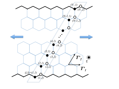
Figure 8: The zigzag slab with lattice vectors $\bm{T}^{\prime}_{1}=(1,0,0)$, $\bm{T}^{\prime}_{2}=(1/2,\sqrt{3}/2,0)$, and $\bm{z}=(0,0,1)$.

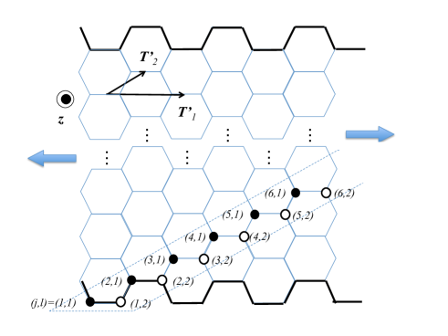
Figure 9: The armchair slab with lattice vectors $\bm{T}^{\prime}_{1}=(1,0,0)$ and $\bm{T}^{\prime}_{2}=(1/2,1/(2\sqrt{3}),0)$, and $\bm{z}=(0,0,1)$.

References

- (1) G. E. Volovik, The universe in a Helium Droplet (Oxford University Press, New York, 2003).
- (2) M. Yamashita, K. Izumina, A. Matsubara, Y. Sasaki, O. Ishikawa, T. Takagi, M. Kubota, and T. Mizusaki, Phys. Rev. Lett. 101, 025302 (2008).
- (3) Y. Maeno, S. Kittaka, T. Nomura, S. Yonezawa, and K. Ishida, J. Phys. Soc. Jpn. 81, 011009 (2012).
- (4) N. Read and D. Green, Phys. Rev. B 61, 10267 (2000).
- (5) R. Willett, Rep. Prog. Phys. 76, 076501 (2013).
- (6) X. Lin, R. Du, and X. Xie, Nat. Sci. Rev. 1, 564 (2014).
- (7) For a review, see, A. M. Black-Schaffer and C. Honerkamp, J. Phys.: Condens. Matter 26, 423201 (2014).
- (8) M. L. Kiesel, C. Platt, W. Hanke, and R. Thomale, Phys. Rev. Lett. 111 097001 (2013).
- (9) Y. Nishikubo, K. Kudo, and M. Nohara, J. Phys. Soc. Jpn. 80, 055002 (2011).
- (10) J. Goryo, M. H. Fischer, and M. Sigrist, Phys. Rev. B 86, 100507(R) (2012).
- (11) P. K. Biswas, H. Luetkens, T. Neupert, T. Stürzer, C. Bains, G. Pascua, A. P. Schnyder, M. H. Fischer. J. Goryo, M. R. Lees, H. Maeter, F. Brückner, H.-H. Klauss, M. Nicklaus, P. J. Baker, A. D. Hillier, M. Sigrist, A. Amato, and D. Johrendt, Phys. Rev. B 87, 180503(R) (2013).
- (12) M. H. Fischer, T. Neupert, C. Platt, A. P. Schnyder, W. Hanke, J. Goryo, R. Thomale, and M. Sigrist, Phys. Rev. B 89, 020509(R) (2014); ibid. 90, 099902 (2014).
- (13) M. H. Fischer, and J. Goryo, J. Phys. Soc. Jpn. 84, 054705 (2015); ibid. 86, 068001 (2017).
- (14) The discussion on the pairing symmetry of SrPtAs is still controversial. See Refs. Wang-Yang-Wang ; Matano-etal ; Landaeta-etal .
- (15) W.-S. Wang, Y. Yang, and Q.-H. Wang, Phys. Rev. B 90, 094514 (2014).
- (16) K. Matano, K. Arima, S. Maeda, Y. Nishikubo, K. Kudo, M. Nohara, and G.-q. Zheng, Phys. Rev. B 89, 140504(R) (2014).
- (17) J. F. Landaeta, S. V. Taylor, I. Bonalde, C. Rojas, Y. Nishikubo, K. Kudo, and M. Nohara, Phys. Rev. B 93, 064504 (2016).
- (18) C. L. Kane and E. J. Mele, Phys. Rev. Lett. 95, 146802 (2005); ibid. 95, 226801 (2005).
- (19) We should make a remark about the surface charge current. It has been pointed out that the surface charge current in a non--wave chiral superconductors is absent in the rotationally symmetric (continuum) system. In a lattice system, however, the surface current survives when the chiral pairing state is supported by the point group symmetry such as in our system Kalline ; Tada-Nie-Oshikawa .
- (20) W. Huang, E. Taylor, and C. Kallin, Phys. Rev. B 90, 224519 (2014).
- (21) Y. Tada, W. Nie, and M. Oshikawa, Phys. Rev. Lett. 114, 195301 (2015).
- (22) Y. Imai, K. Wakabayashi, and M. Sigrist, Phys. Rev. B 85, 174532 (2012); ibid. 88, 144503 (2013).
- (23) A. Schnyder, S. Ryu, A. Furusaki, and A. W. W. Ludwig, Phys. Rev. B 78, 195125 (2008).
- (24) S.J. Youn, M. H. Fischer, S. H. Rhim, M. Sigrist, and D. F. Agterberg, Phys. Rev. B 85 220505 (2012).
- (25) Y. Yanase, and K. Shiozaki, Phys. Rev. B 95, 224514 (2017).
- (26) F.-f. Zhu, W.-j. Cheng, Y. Xu, C.-l. Gao, D.-d. Guan, C.-h. Liu, D. Qian, S.-C. Zhang, and J.-f. Jia, Nature Materials 14, 1020 (2015).
- (27) Zhe Wang, D.-K. Ki, H. Chen, H. Berger, A. H. MacDonald, and A. F. Morpurgo, Nat. Commun. 6, 8339 (2015).
- (28) T. Kimura, Y. Otani, T. Sato, S. Takahashi, and S. Maekawa, Phys. Rev. Lett. 98, 156601 (2007); ibid. 249901 (2007).
- (29) D. Maruyama, M. Sigrist, and Y. Yanase, J. Phys. Soc. Jpn. 81 034702 (2012).
- (30) For a review, see M. Sato and Y. Ando, Rep. Prob. Phys. 80, 076501 (2017).
- (31) M. Nohara (private communication).