Exotic Bifurcations Inspired by Walking Droplet Dynamics

Abstract

We identify two rather novel types of (compound) dynamical bifurcations generated primarily by interactions of an invariant attracting submanifold with stable and unstable manifolds of hyperbolic fixed points. These bifurcation types - inspired by recent investigations of mathematical models for walking droplet (pilot-wave) phenomena - are introduced and illustrated. Some of the one-parameter bifurcation types are analyzed in detail and extended from the plane to higher-dimensional spaces. A few applications to walking droplet dynamics are analyzed.

1 Introduction

Inspired by our recent research on the dynamical properties of mathematical models of walking droplet (pilot-wave) phenomena [16], we shall describe and analyze what appear to be new types or classes of bifurcations. Owing largely to its potential for producing macroscopic analogs of certain quantum phenomena, walking droplet dynamics has become a very active area of research since the seminal work of Couder et al. [5]. In this study we focus on the dynamical systems models arising from walking droplets, interesting examples of which can be found in Gilet [7], Milewski et al. [9], Oza et al. [14], Rahman and Blackmore [16], and Shirokov [19]. Furthermore, a detailed summary of recent advancements in hydrodynamic pilot-waves can be found in [4]. Simulations of the solutions of some of the mathematical models for walkers are not only interesting for their quantum-like effects, they exhibit exotic bifurcations that are apt to attract the interest of dynamical systems researchers and enthusiasts. In particular, the two-parameter planar discrete dynamical systems model of Gilet [7] of the form $G:\mathbb{R}^{2}\rightarrow\mathbb{R}^{2}$ defined as

$$G(x,y;C;\mu):=\left(x-C\Psi^{\prime}(x)y,\mu(y+\Psi(x))\right),$$ (1)

where $0<C,\mu<1$ are parameters and $\Psi$ is an odd, $2\pi$-periodic function given by

$$\Psi(x):=\frac{1}{\sqrt{\pi}}\left(\cos\beta\sin 3x+\sin\beta\sin 5x\right),$$

where $\beta$ is usually chosen to be $\pi/3$ or $\pi/6$, exhibits not only Neimark–Sacker bifurcations, but more exotic chaotic bifurcations that have apparently not been analyzed in detail in the literature. Simulations of the dynamics of (1) have shown that these exotic bifurcations are similar in certain respects if one of the parameters $C,\mu$ is varied and the other fixed, but also quite different in other ways. For example, in the $C$ fixed case shown in Fig. 1 , we see a progression of similarly shaped attractors ending in what appears to be a chaotic state. Actually, if $\mu$ is increased further (not shown), the chaotic attractor exhibits dramatic changes, which are apparently due to a series of dynamical crises (cf. Ott [13]).

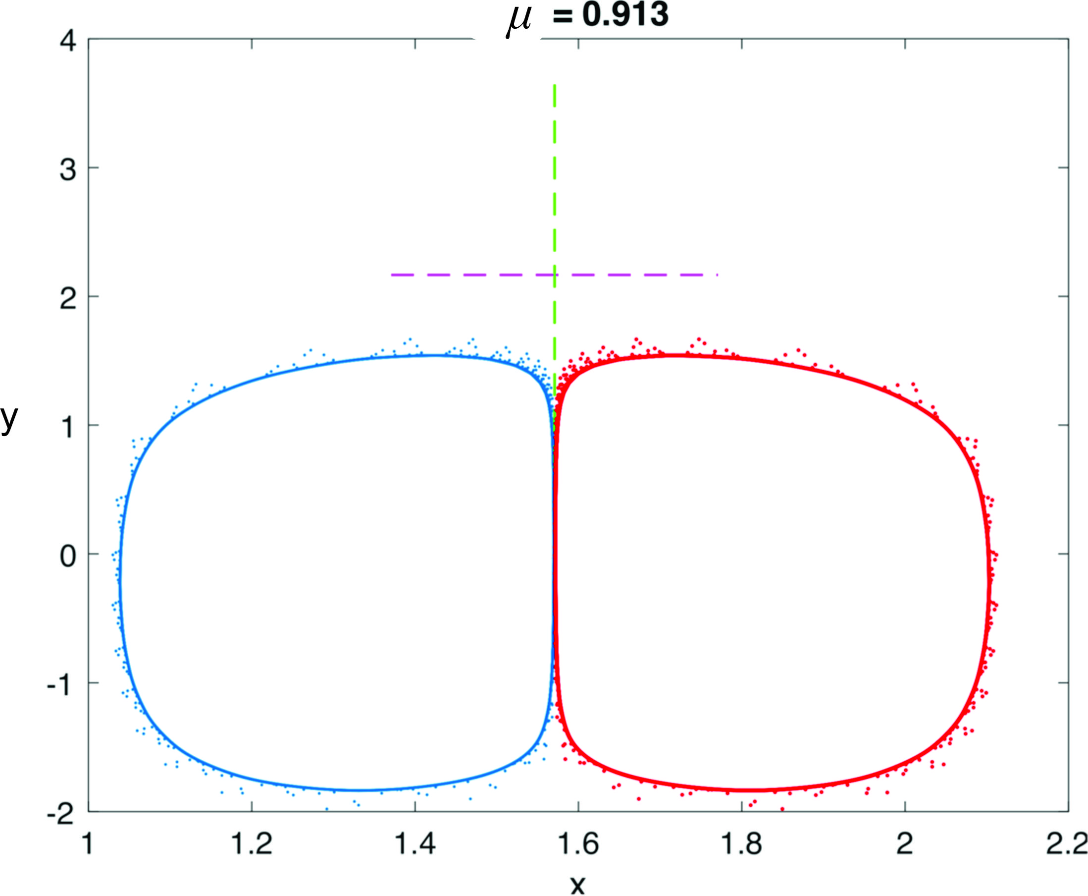
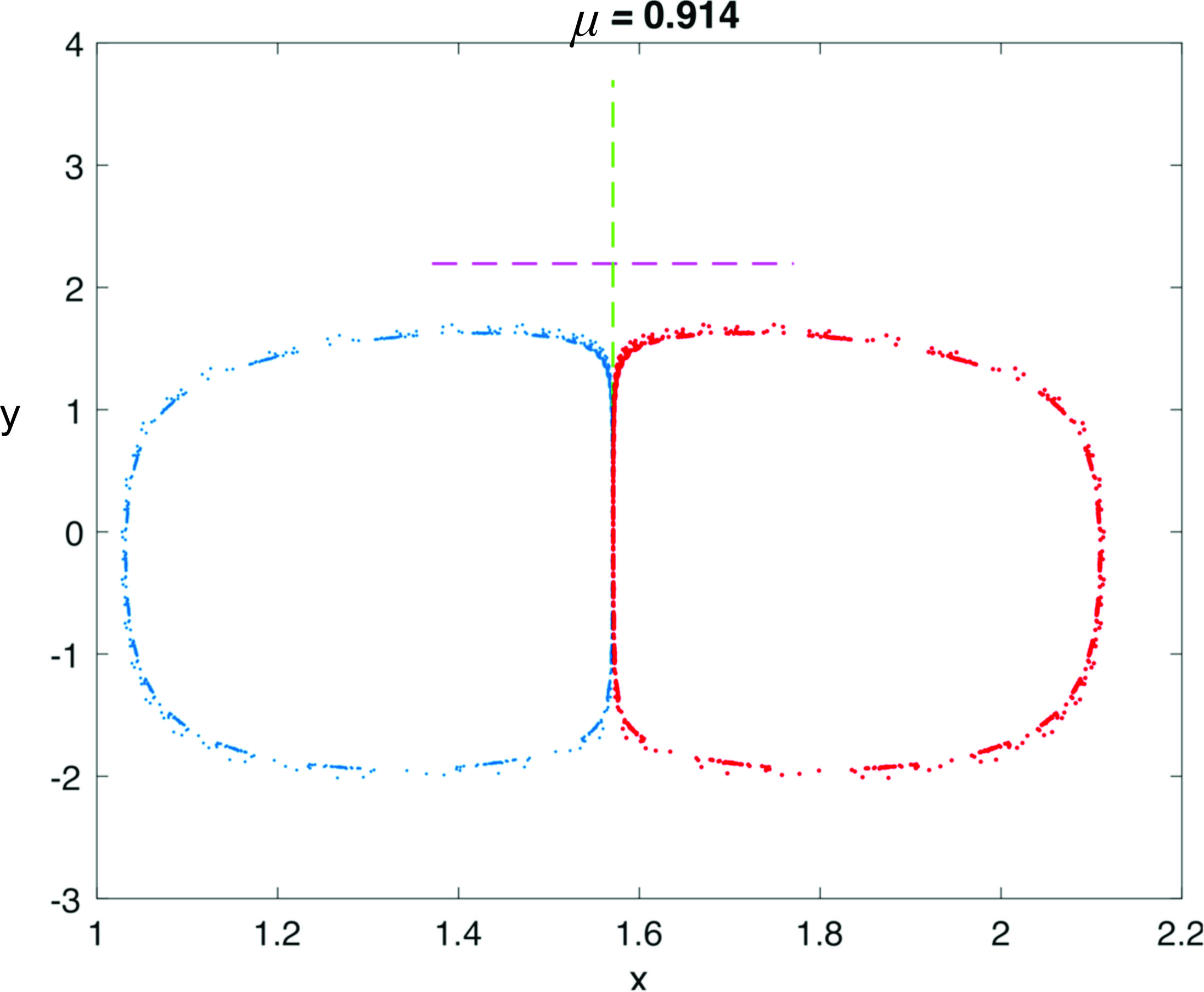
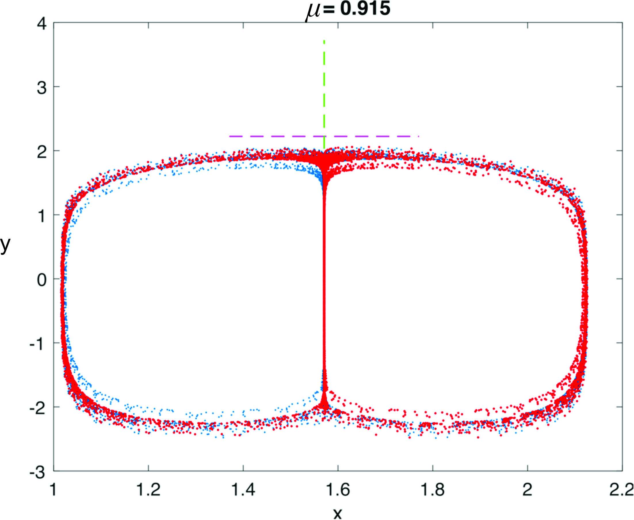
Figure 1: Bifurcation evolution for fixed $C$ (increasing $\mu$).

On the other hand, in Fig. 2 we show a sequence in which $\mu$ is fixed and $C$ varied from $0.45$ to $0.528$ at which point we see what appears to be a chaotic strange attractor. This chaotic strange attractor actually persists in shape up to around $C=0.7$ (not shown). Beyond $0.7$ (also not shown) the attractor changes in shape more or less continuously until it finally breaks up into a chaotic splatter with just a ghost-like shadow of the prior shape - a last stage that is also indicative of dynamical crises. In this investigation, we concentrate on abstracting the bifurcation properties of the Gilet map associated with fixing $\mu$ and varying $C$.

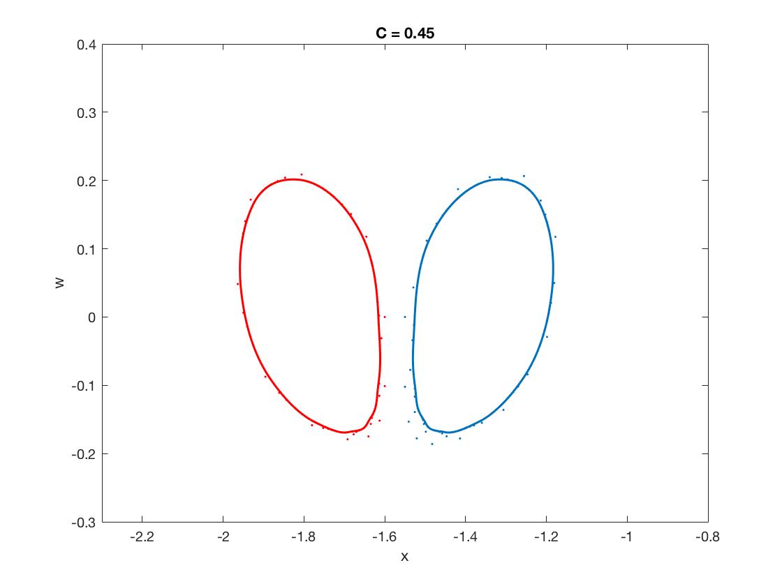
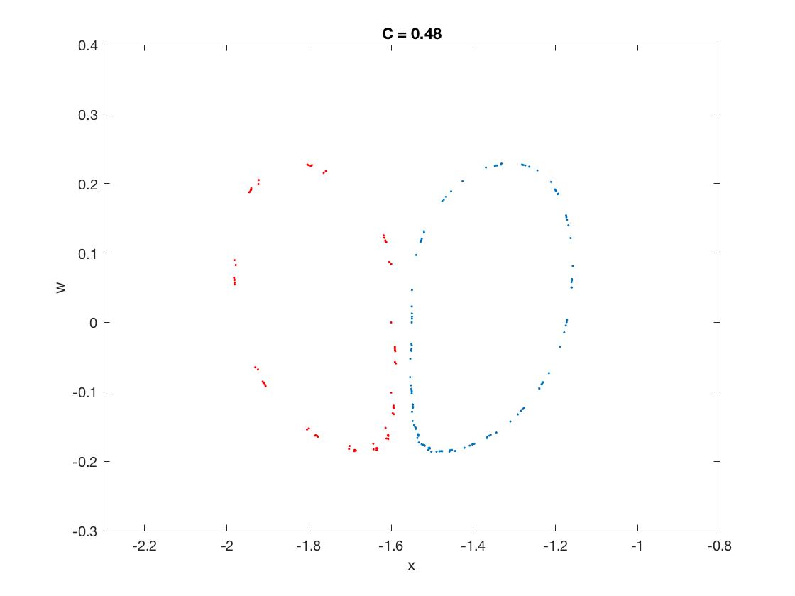
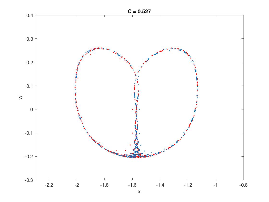
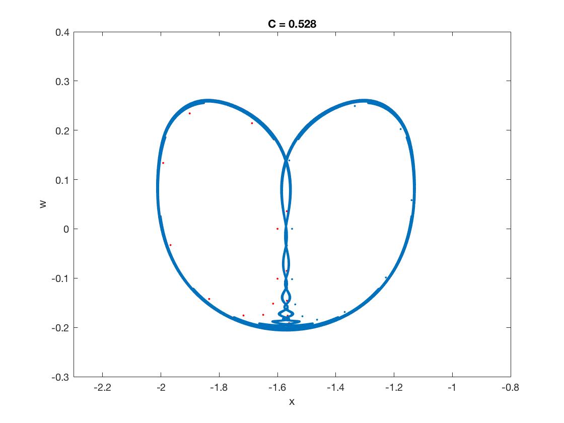
Figure 2: Bifurcation evolution for fixed $\mu$ (increasing $C$).

The bifurcations that we describe in the sequel are those for discrete dynamical systems comprising the iterates of differentiable, parameter-dependent self-maps of smooth finite-dimensional manifolds, and they are generated by interactions of closed (positively) invariant submanifolds with stable and unstable manifolds of saddle points as a single parameter is varied. In the interest of simplicity and clarity, we shall confine our attention to maps $f\in C^{1}\left(\mathbb{R}^{m}\times\mathbb{R},\mathbb{R}^{m}\right)$, where $m$ is a natural number (in $\mathbb{N}$) and, as usual,

$$C^{1}\left(\mathbb{R}^{m}\times\mathbb{R},\mathbb{R}^{m}\right):=\left\{f:\mathbb{R}^{m}\times\mathbb{R}\rightarrow\mathbb{R}^{m}:f\text{ is continuously differentiable}\right\}.$$

Here, of course, $\mathbb{R}^{m}$ and $\mathbb{R}$ are, respectively, Euclidean $m$- and $1$-space, which represent the phase and parameter spaces of the dynamical system and points in $\mathbb{R}^{m}\times\mathbb{R}$ to be denoted as $(\boldsymbol{x},\mathbb{\sigma})$. An example of the kind of map we shall be investigating is that of the form of (1) with $\mu$ a fixed constant in $(0,1)$ and the other parameter $C$, which we denote as $\sigma$, varying in $(0,1)$; namely,

$$F(x,y;\sigma):=\left(x-\sigma\Psi^{\prime}(x)y,\mu(y+\Psi(x))\right),$$ (2)

In what follows, we assume a knowledge of the fundamentals of modern dynamical systems theory such as can be found in [2, 13, 15, 17, 24]. Our main results are detailed in the remainder of this paper, which is arranged as follows. In Section 2 and Section 3 we describe the planar forms of the bifurcations involving the interaction of an attracting invariant Jordan curve and stable and unstable manifolds of saddle points. These bifurcations share some features with the dynamical phenomena described in Aronson et al. [1] and Frouzakis et al. [6], but they appear to be essentially new. More specifically, in Section 2, we introduce and analyze planar dynamical bifurcations generated by the interaction of an attracting Jordan curve and the stable manifold of a saddle point. In particular, the interaction first induces a bifurcation caused by a tangent homoclinic orbit, which is followed by a sequence of additional tangent homoclinic orbits interspersed with transverse homoclinic orbits as the parameter is increased. Ultimately, however, an increase in $\sigma$ leads to a final tangent homoclinic orbit after which there is a parameter interval on which there a robust chaotic strange attractor, which is amenable to abstraction. As mentioned above, there are additional types of bifurcations for larger parameter values, which shall not be described in detail here. It should be noted that the bifurcations considered in this paper, which shall be designated as being of type 1, are directly related to those of the Gilet map (1) where a slice-like region of non-injectivity of the map plays a key role. There is a second type - a variant of the Gilet map - where the map is a diffeomorphism that produces analogous bifurcations, which we shall analyze in a forthcoming paper.

Section 3 is where we describe a modification of the bifurcation in the preceding section generated by the interaction of an attracting Jordan curve with a pair of stable manifolds, which can induce heteroclinic cycles that generate chaotic strange attractors followed by homoclinic bifurcations. Next, in Section 4, we discuss some higher-dimensional analogs of the planar bifurcations analyzed in the preceding sections. In Section 5, we describe several applications and examples of the bifurcations, with a focus on the phenomena and mathematical models that inspired our work on the bifurcations; namely, walking droplet dynamics. Finally, in Section 6, we summarize some of the conclusions reached in this research and adumbrate possible related future work, which includes analyzing the bifurcations in the dynamics of the map (1) when $C$ is fixed and $\mu$ varied.

2 Homoclinic Bifurcations of Type 1 in the Plane

In this and the next section, we restrict our attention to a $C^{1}$ map $f:\mathbb{R}^{2}\times\mathbb{R}\rightarrow\mathbb{R}^{2}$, with the tacit understanding that we could have just as well considered a 1-parameter dependent map on a simply-connected open subset of a smooth surface. The points of $\ \mathbb{R}^{2}\times\mathbb{R}$ shall be denoted by $(\boldsymbol{x},\sigma)=\left((x,y),\sigma\right)$ and we use the standard notation $f_{\sigma}:\mathbb{R}^{2}\rightarrow\mathbb{R}^{2}$ for the planar map with the parameter $\sigma$ fixed at a particular value in $(0,1)$.

Let us set the stage for the homoclinic bifurcation of type $1$ with more specificity. For this, we assume that $\boldsymbol{p}(\sigma):=(\hat{x}(\sigma),\hat{y}(\sigma))$ is a saddle point of $f_{\sigma}$, with one eigenvalue $\lambda^{u}(\sigma)>1$ and the other $0<\lambda^{s}(\sigma)<1$ for all $\sigma\in[a,b)\subset(0,1)$ such that $\hat{x}(a),\hat{y}(a)>0$, where $a<b$ . We may also assume that the linear unstable manifold is horizontal when $\sigma=a$; i.e., $W_{lin}^{u}(\boldsymbol{p}(a))$ is the line $y=\hat{y}(a)$. In addition, we assume that the saddle point, although it may move as the parameter is varied, remains within the open rectangle $R_{\alpha,\beta}:=(0,\hat{x}(a)+\alpha)\times(0,\hat{y}(a)+\beta)$ for some $\alpha,\beta>0$ and all $a\leq\nu<b$, and its stable manifold $W^{s}(\boldsymbol{p}(\sigma))$ lies in the open vertical strip $V_{\alpha}:=(0,\hat{x}(a)+\alpha)\times\mathbb{R}$ for all $a\leq\sigma<1$.

A principal feature of the bifurcation is an attracting invariant closed tubular neighborhood $T(\sigma)$ of a $C^{1}$ closed Jordan curve $C=C(\sigma)$, which we call an invariant tube with center $C$ for the map. Then there is for some $\sigma$ an associated compact invariant attracting set

$$\mathfrak{C}\mathcal{(\sigma)}:={\displaystyle\bigcap\nolimits_{n=1}^{\infty}}f_{\sigma}^{n}\left(T(\sigma)\right),$$

which, for an appropriately chosen center, is equal to $C(\sigma)$ for some initial subinterval of $[a,b)$. It should be noted that such invariant circles and tubes rather frequently arise from Neimark–Sacker bifurcations of sinks, especially those of the spiral variety (cf. [11, 18] and also [2, 17, 24]). We also assume that for the parameter values for which the invariant tubes exist, $T(\sigma)$ is contained in the open rectangle $\mathcal{R}_{\alpha,\beta}:=\{(x,y):\left|x\right|<\hat{x}(a)+\alpha,\left|y\right|<\hat{y}(a)+\beta\}$ , and even more; it is contained in the set $Q(\sigma)$ comprising all points in $\mathcal{R}_{\alpha,\beta}$ to the left of $W^{s}(\boldsymbol{p}(\sigma))$ and beneath $W_{lin}^{u}(\boldsymbol{p}(\sigma))$, respectively. Moreover, we assume that $f_{\sigma}$ has a positive (counterclockwise) rotation number in the sense that the iterates of any normal section of $T(\sigma)$ completely traverse the tube in a counterclockwise manner.

Finally, there is another important feature for maps of the type represented by Gilet’s model. Namely, it is assumed that there is a $a<\sigma_{\#}<b$ such that for all $\sigma\in[a,\sigma_{\#})$, the basin of attraction of $\mathfrak{C}(\sigma)$ contains all points $(x,y)$ in $\mathcal{R}_{\alpha,\beta}$ to the left of $W^{s}(\boldsymbol{p}(\sigma))$, except for points in a curvilinear slice $Z(\sigma)$ below the saddle point with one edge and the image under $f_{\sigma}$ of the other edge contained in $W^{s}(\boldsymbol{p}(\sigma))$, having the the property that $f_{\sigma}$ flips its interior across the stable manifold. This slice is a key agent in producing a chaotic strange attractor as the center of the tube expands for Gilet-type maps.

Now that the contextual foundation has been established, we shall prove a result describing the homoclinic type bifurcations that we have in mind. Toward this end, it is useful to summarize the descriptions above in the form of a list of detailed but reasonably succinct properties. These attributes of the map $f:\mathbb{R}^{2}\times\mathbb{[}a,b)\rightarrow\mathbb{R}^{2}$, illustrated in Fig. 3, are as follows:

• $f\in C^{1}:=C^{1}\left(\mathbb{R}^{2}\times\mathbb{[}a,b),\mathbb{R}^{2}\right)$, where $\mathbb{[}a,b)\subset(0,1)$ and $f_{\sigma}$ has a single saddle point $\boldsymbol{p}(\sigma):=(\hat{x}(\sigma),\hat{y}(\sigma))$, which is such that: (i) $\hat{x}(a),\hat{y}(a)>0$; (ii) there are real constants $\kappa_{s}$, $\kappa_{u}$ such that the eigenvalues $\lambda^{s}(\sigma)$ and $\lambda^{u}(\sigma)$ of $f_{\sigma}^{\prime}\left(\boldsymbol{p}(\sigma)\right)$ satisfy $0<\lambda^{s}(\sigma)\leq\kappa_{s}<1<\kappa_{u}\leq\lambda^{u}(\sigma)$ for all $a\leq\sigma<b$; (iii) the eigenvector corresponding to $\lambda^{u}(a)$ is parallel to the $x$-axis; (iv) there is a vertical strip of the form

  $$V_{\alpha}:=\{\boldsymbol{x}:=(x,y)\in\ \mathbb{R}^{2}:0<x<\hat{x}(a)+\alpha\}$$

  for some $\alpha>0$ such that the stable manifold $W^{s}(\boldsymbol{p}(\sigma))\subset S_{\alpha}$ for all $a\leq\sigma<b$ and separates the plane into left and right components denoted as $K_{-}(\sigma)$ and $K_{+}(\sigma)$, respectively; and (v) there is a $\beta>0$ such that

  $$\boldsymbol{p}(\sigma)\in R_{\alpha,\beta}:=\{(x,y)\in\ \mathbb{R}^{2}:0<x<\hat{x}(a)+\alpha,0<y<\hat{y}(a)+\beta\}$$

  $$\subset\mathcal{R}_{\alpha,\beta}:=\{(x,y):\left|x\right|<\hat{x}(a)+\alpha,\left|y\right|<\hat{y}(a)+\beta\}$$

  for all $\sigma\in[a,b)$.

• There exist $a<\sigma_{1}\leq\sigma_{\#}<\sigma_{t}<\sigma_{2}<\sigma_{3}<b$ such that the following obtain: (i) there is a (positively) $f_{\sigma}$-invariant attracting tubular neighborhood $T(\sigma)$ of a $C^{1}$ closed Jordan curve $C(\sigma)$ for all $\sigma\in[a,\sigma_{2})$; (ii) $f_{\sigma}$ restricted to $T(\sigma)$ has a positive (counterclockwise) rotation number for all $\sigma\in[a,\sigma_{2})$; (iii) the closed curve can be chosen so that centerset

  $$\mathfrak{C}(\sigma):={\displaystyle\bigcap\nolimits_{n=1}^{\infty}}f_{\sigma}^{n}\left(T(\sigma)\right)=C(\sigma)$$

  for all $\sigma\in[a,\sigma_{1})$; (iv) $T(\sigma)\subset K_{-}(\sigma)\cap\mathcal{R}_{\alpha,\beta}\cap H(\sigma)$, where $H(\sigma)$ is the half-plane defined by $y<\hat{y}(\sigma)$, for all $\sigma\in[a,\sigma_{2})$; (v) $\mathfrak{C}(\sigma)$ is a nonempty attracting set for all $\sigma\in[a,\sigma_{\#})\cup[\sigma_{2},\sigma_{3})$ and has an open basin of attraction, denoted as $\mathfrak{\mathring{B}}(\sigma)$, containing $\left(K_{-}(\sigma)\cap\mathcal{R}_{\alpha,\beta}\cap\mathfrak{C}_{\mathrm{ext}}(\sigma)\right)\smallsetminus Z(\sigma)$ and $\mathfrak{C}(\sigma)\cap Z(\sigma)=\varnothing$  for all $\sigma\in[a,\sigma_{\#})$, where $\mathfrak{C}_{\mathrm{ext}}(\sigma)$ is the exterior of the centerset and $Z(\sigma)$ is a set defined as follows: There is for every $\sigma\in[a,b)$ an orientation preserving $C^{1}$-diffeomorphism $\Phi_{\sigma}$ of an open neighborhood $U_{\sigma}$ of a portion of $W^{s}(\boldsymbol{p}(\sigma))$ below $\boldsymbol{p}(\sigma)$ such that

  $$\Phi_{\sigma}\left(Z(\sigma)\right):=\left\{(\xi,\eta):-1\leq\xi\leq 0,\eta\leq\varphi(\xi)\right\},$$

  where $\varphi:[-1,1]\rightarrow(-1,0]$ is a $C^{1}$ function such that $\varphi(0)=0$ and $\varphi^{\prime}(\xi)>0$ when $\xi<0$. Moreover, the right-hand bounding curve $c_{r}(\sigma):=\Phi_{\sigma}^{-1}\left(\left\{(0,\eta):\varphi(-1)\leq\eta\leq 0\right\}\right)$ and the $f_{\sigma}$ image of left-hand bounding curve $c_{l}(\sigma):=\Phi_{\sigma}^{-1}\left(\left\{\left(\xi,\varphi(\xi)\right):-1\leq\xi\leq 0\right\}\right)$ lies in $W^{s}(\boldsymbol{p}(\sigma))$, while $f_{\sigma}$ maps the interior $\mathring{Z}(\sigma)$ into $K_{+}(\sigma)$.

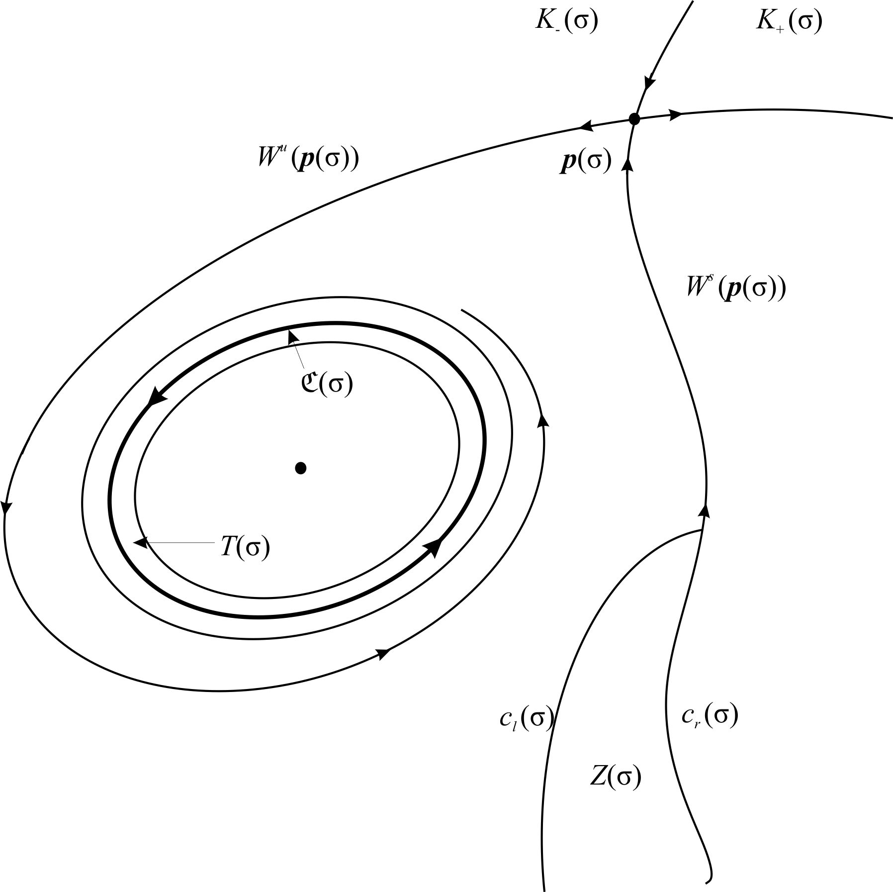
Figure 3: Topography of the homoclinic type 1 bifurcation

We have now sufficiently prepared the way for the statement and proof of our first main result based on the above assumptions, which concerns the existence of what we call a homoclinic type $1$ bifurcation. However, it is convenient to first introduce the following definition: The left unstable manifold is

$$W_{l}^{u}(\boldsymbol{p}(\sigma)):={\displaystyle\bigcup\nolimits_{n=1}^{\infty}}f_{\sigma}^{n}\left(\left\{\boldsymbol{x}\in W^{u}(\boldsymbol{p}(\sigma)):\boldsymbol{x}\in\{\boldsymbol{p}(\sigma)\}\cup K_{-}(\sigma)\text{ and }d\left(\boldsymbol{x},\boldsymbol{p}(\sigma)\right)\leq\nu\,\forall\,\nu>0\text{ }\right\}\right).$$

Theorem 1.

Let $f:\mathbb{R}^{2}\times[a,b)\rightarrow\mathbb{R}^{2}$ satisfy (A1) and (A2) and the additional property:

• The distance $\Delta(\sigma):=\mathrm{dist}\left(\mathfrak{C}(\sigma),Z(\sigma)\right):=\inf\left\{\left|\boldsymbol{x}-\boldsymbol{y}\right|:(\boldsymbol{x},\boldsymbol{y})\in\mathfrak{C}(\sigma)\times Z(\sigma)\right\}$ satisfies
  $\Delta(a)>0$ and is a nonincreasing function of $\sigma$ on $[a,\sigma_{\#})\cup[\sigma_{2},\sigma_{3})$ and $\lim_{\sigma\uparrow\sigma_{3}}\Delta(\sigma)=0$.

Then, there are $a<\sigma_{\#}\leq\sigma_{t}\leq\sigma_{2}\leq\sigma_{\ast}<\sigma_{3}<b_{1}<1$, where $\sigma_{t}$ and $\sigma_{\ast}$ are the first and last, respectively, values of $\sigma$ where there is a tangent intersection of the stable and unstable manifolds of $\boldsymbol{p}(\sigma)$ such that for all $\sigma_{\ast}<\sigma<b_{1}$, $f_{\sigma}$ has a chaotic strange attractor $\mathfrak{A}(\sigma)$, which is the closure of the left unstable manifold: namely,

$$\mathfrak{A}(\sigma):=\overline{W_{l}^{u}(\boldsymbol{p}(\sigma))}\text{.}$$ (3)

Proof.

We begin by focusing on a tubular type strip $Q=Q(\sigma;\nu)$ for $W^{s}(\boldsymbol{p}(\sigma))$ (excluding $c_{l}(\sigma)$) cut off just above $\boldsymbol{p}(\sigma)$ and below at the lower edge of $R(\alpha,\beta)$ as shown in Fig. 3, with the understanding that the dimensions can be taken to be as small as suits our purposes in what follows. In particular, we take the width of the strip to be $2\nu$ and the top edge to be parallel to and at a distance of $\nu$ above $W^{u}(\boldsymbol{p}(\sigma))$, where $\nu>0$. In this context, we shall find it convenient to define $W_{\nu}^{u}(\sigma)$ to be the closed segment, with interior in $K_{-}(\sigma)$, of the unstable manifold from $\boldsymbol{p}(\sigma)$ to the boundary of $Q$, and to use $s_{\sigma}:=s_{\sigma}(\boldsymbol{x})=s(\boldsymbol{x})$ to denote the arclength from the fixed point to any point $\boldsymbol{x}\in W_{\nu}^{u}(\sigma)$ or any of its $f_{\sigma}$-iterates. We also define for every nonnegative integer $n$ the endpoint $e_{\sigma}^{n}$, to be the boundary point of the $C^{1}$-submanifold (with boundary) $\mathcal{W}_{\sigma}^{u}(\sigma,n):=f_{\sigma}^{n}(W_{\nu}^{u}(\sigma))$ for which $s_{\sigma}$ is positive and actually increases without bound as $n\rightarrow\infty$ as long as $\sigma<\sigma_{\#}$.

The idea of the proof is illustrated rather simply in Figs. 3 and 4, but some technical details are necessary. It follows from the hypotheses (A1)-(A3) that for any $\nu>0$ there is a positive integer $N=N_{\nu}(\sigma)$ and a first $\sigma=\sigma_{t}\in[a,\sigma_{2})$ such that $\mathcal{W}_{\nu}^{u}(\sigma,N)$ is tangent to $c_{l}(\sigma)$, which implies that $\mathcal{W}_{\nu}^{u}(\sigma_{t},N+1)$ is tangent to $W^{s}(\boldsymbol{p}(\sigma_{t}))$. Then, as $\sigma$ is increased, there must be a last value, $\sigma_{\ast}$, with $\sigma_{t}\leq\sigma_{\ast}<\sigma_{2}$, such that $\mathcal{W}_{\nu}^{u}(\sigma,N)$ crosses $c_{l}(\sigma)$ into the interior of $Z(\sigma)$, implying that $Q_{l,\sigma}(\omega,N+1):=$ $f_{\sigma}^{N+1}(Q_{-}(\sigma;\nu))$, where $Q_{-}(\sigma;\nu):=Q(\sigma;\nu)\cap\overline{K_{-}(\sigma)}$, which contains a portion of $\mathcal{W}_{\nu}^{u}(\sigma,N+1)$, actually crosses over $Q(\sigma;\nu)$ into $K_{+}(\sigma)$ for all sufficiently small $\nu>0$ whenever $\sigma_{\ast}<\sigma$. As a consequence of this situation, called an $\times$-crossing, the desired result follows from the attracting horseshoe theorem in [8], which incorporates the geometric chaos and fractal set arguments of Birkhoff–Moser–Smale theory (cf. [2, 10, 15, 17, 20, 24]). In particular, there is an attracting horseshoe in $f_{\sigma}^{N+1}(Q)$, which is depicted in Fig. 4(c), which persists as long as $\sigma_{\ast}<\sigma<b_{1}$, where $\sigma=b_{1}$ is the first parameter value where the unstable manifold has a tangent intersection with the stable manifold in $Z(\sigma)$.

∎

The proof of Theorem 1 actually yields more information than provided in the statement; for example, it explains the “blinking effect” observed for the attractor as $\sigma:=C$ increases. This is caused by a sequence of tangent intersections between the stable and unstable manifolds of the saddle point $\boldsymbol{p}(\sigma)$ - each a bifurcation value in its own right - as described by Newhouse [12], which proves the following result.

Corollary 1.

Let $f$ be as in Theorem $1$. Then the bifurcation value $\sigma_{\ast}$ precipitating the creation of a robust stable chaotic strange attractor for $\sigma_{\ast}<\sigma<b_{1}$, is proceeded by a sequence of bifurcation values $\sigma_{t}<\sigma_{t(1)}<\sigma_{t(2)}<\cdots<\sigma_{\ast}$ corresponding to successive tangent intersections between the stable and unstable manifolds of the saddle point as $\sigma$ increases.

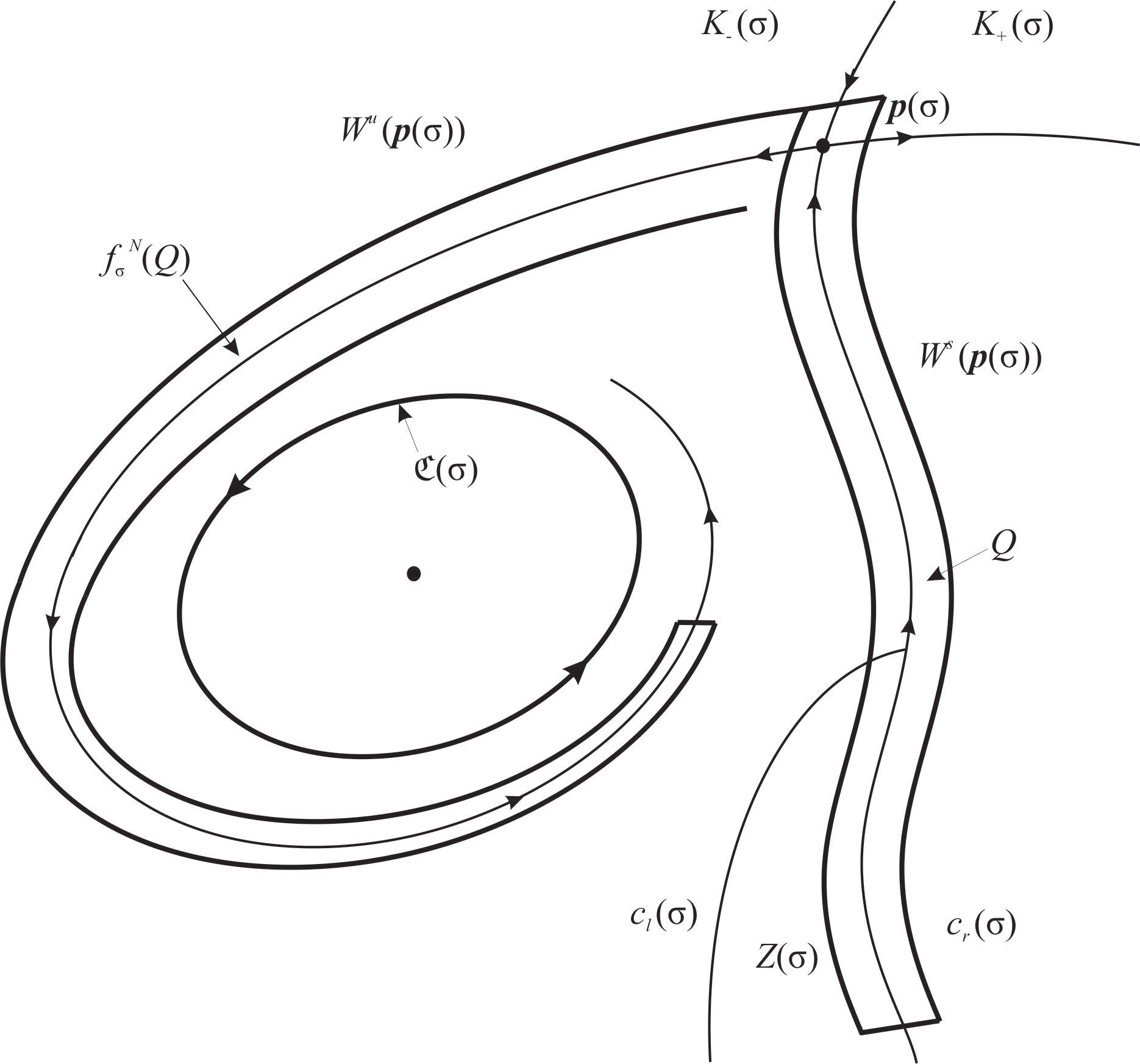
(a) $\sigma<\sigma_{t}$

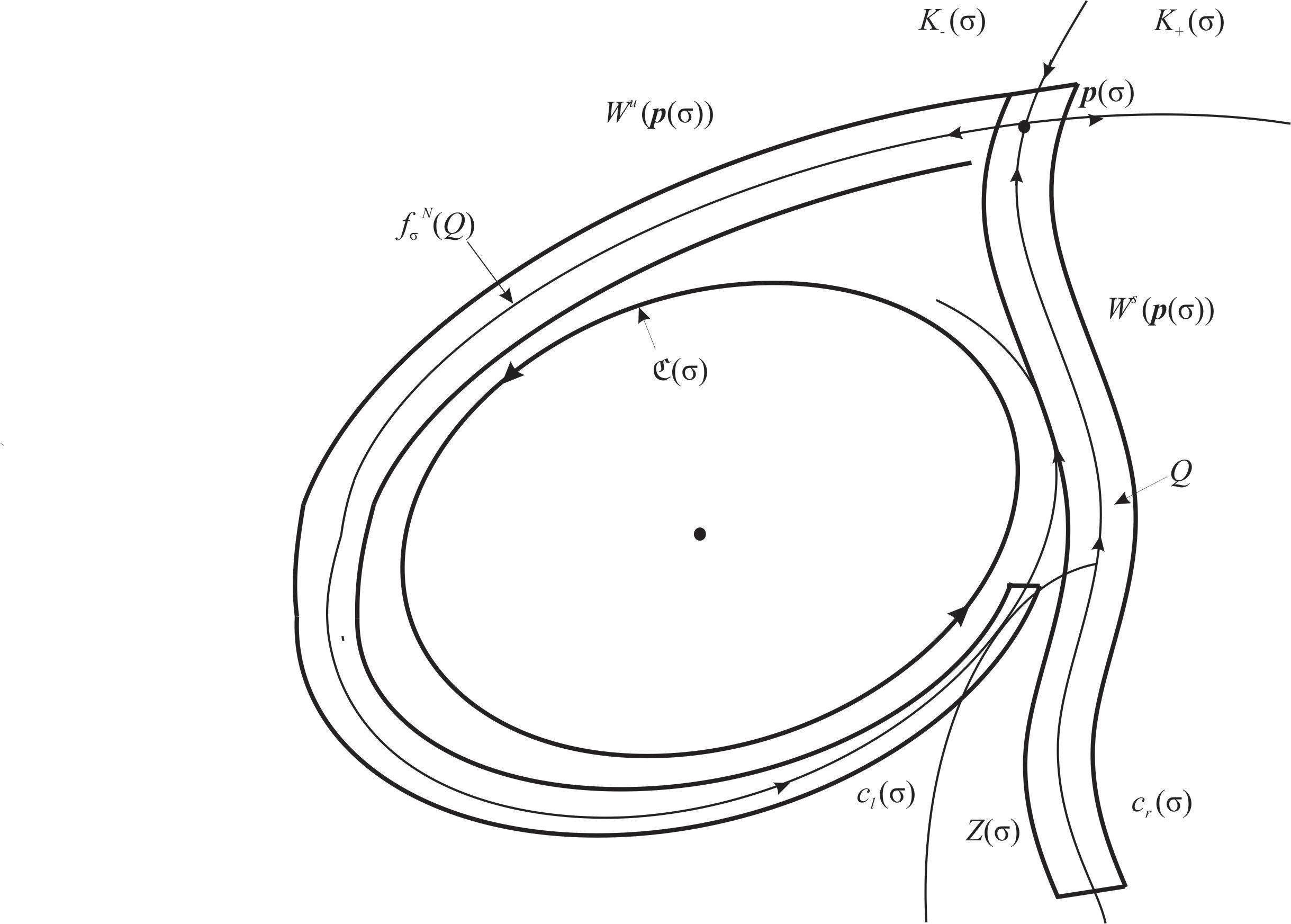
(b) $\sigma=\sigma_{t}$

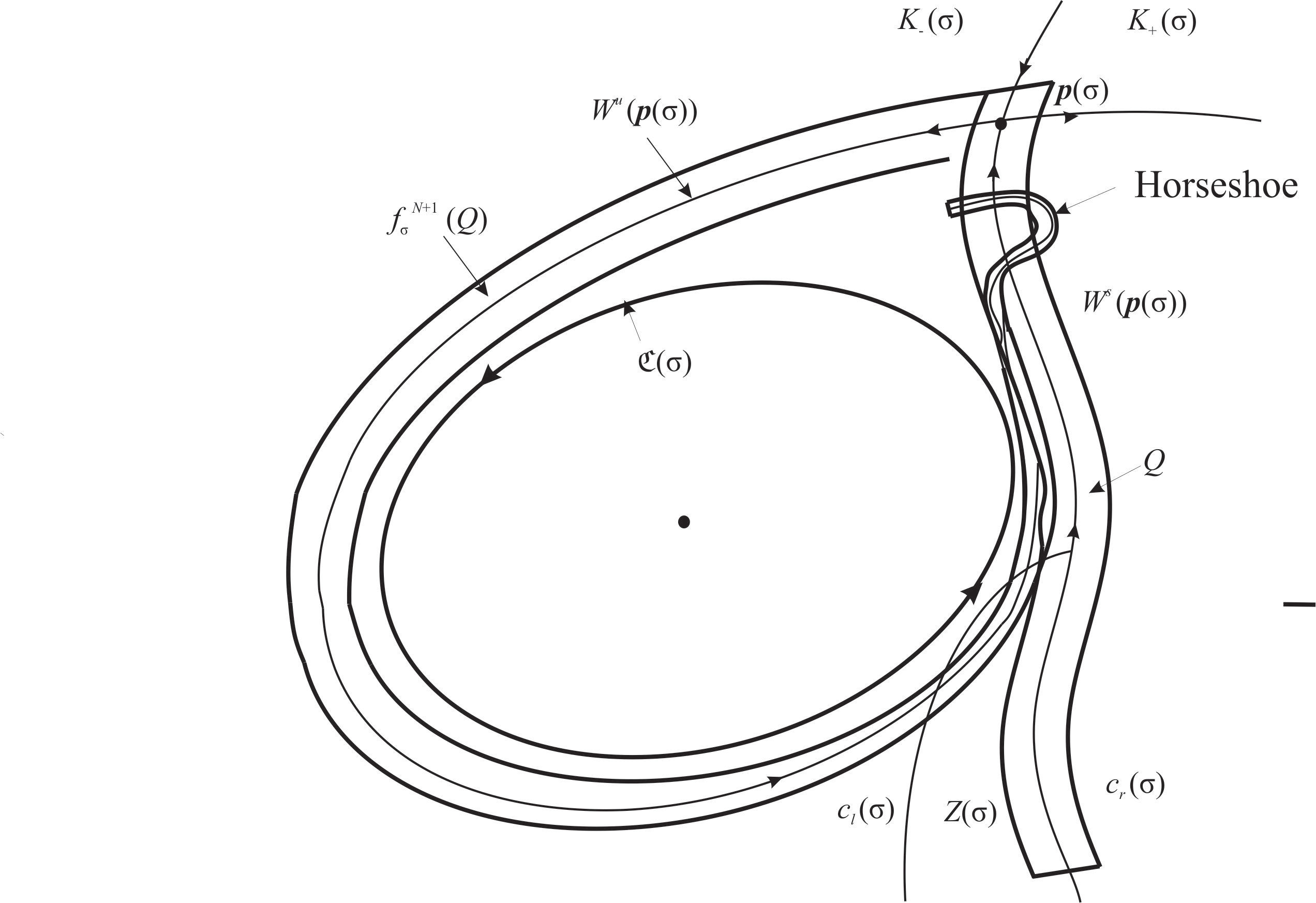
(c) $\sigma_{*}<\sigma<b_{1}$

Figure 4: Geometric evolution of the homoclinic type-1 bifurcation.

3 Heteroclinic-Homoclinic Bifurcations of Type 1 in the Plane

Next, we consider a combined heteroclinic and homoclinic variant of the bifurcation in Section 2, illustrated in Fig. 5, that involves a pair of saddle points, which we set up first with the appropriate analogs of properties (A1) and (A2).

• $f\in C^{1}:=C^{1}\left(\mathbb{R}^{2}\times\mathbb{[}a,b),\mathbb{R}^{2}\right)$ and $f_{\sigma}$ has a pair of saddle points $\boldsymbol{p}(\sigma):=(\hat{x}(\sigma),\hat{y}(\sigma))$ and $\boldsymbol{q}(\sigma):=(\breve{x}(\sigma),\breve{y}(\sigma))$, which are such that: (i) $\boldsymbol{p}(\omega)$ is in the first quadrant and $\boldsymbol{q}(\omega)$ is in the third quadrant of $\mathbb{R}^{2}$ for all $a\leq\sigma<b$ ; (ii) there real constants $\kappa_{s}$, $\kappa_{u}$ such that the eigenvalues $\hat{\lambda}^{s}(\sigma)$ and $\hat{\lambda}^{u}(\sigma)$ of $f_{\sigma}^{\prime}\left(\boldsymbol{p}(\sigma)\right)$ and $\tilde{\lambda}^{s}(\sigma)$ and $\tilde{\lambda}^{u}(\sigma)$ of $f_{\sigma}^{\prime}\left(\boldsymbol{q}(\omega)\right)$ satisfy $0<\hat{\lambda}^{s}(\sigma),\tilde{\lambda}^{s}(\sigma)\leq\kappa_{s}<1<\kappa_{u}\leq\hat{\lambda}^{u}(\sigma),\tilde{\lambda}^{u}(\sigma)$ for all $a\leq\sigma<b$; (iii) the eigenvectors corresponding to $\hat{\lambda}^{u}(a)$ and $\tilde{\lambda}^{u}(a)$ are parallel to the $x$-axis; (iv) there is a vertical strip of the form

  $$S_{\alpha}:=\{\boldsymbol{x}\in\ \mathbb{R}^{2}:\breve{x}(a)-\alpha<\left|x\right|<\hat{x}(a)+\alpha\}$$

  for some $\alpha>0$ such that the stable manifolds $W^{s}(\boldsymbol{p}(\sigma)),W^{s}(\boldsymbol{q}(\sigma))\subset S_{\alpha}$ for all $a\leq\sigma<b$ and separates the plane into left, middle and right components denoted as $K_{-}(\sigma)$, $K(\sigma)$ and $K_{+}(\sigma)$, respectively; and (v) there is a $\beta>0$ such that

  $$\boldsymbol{p},\boldsymbol{q}\in R(\alpha,\beta):=\{(x,y)\in\ \mathbb{R}^{2}:\breve{x}(a)-\alpha<\left|x\right|<\hat{x}(a)+\alpha,\,\breve{y}(a)-\beta<\left|y\right|<\hat{y}(a)+\beta\}$$

  for all $\sigma\in[a,b)$.

• There exist $a<\sigma_{1}<\sigma_{2}<b$ such that the following obtain: (i) there is a (positively) $f_{\sigma}$-invariant attracting tubular neighborhood $T(\sigma)$ of a $C^{1}$ closed Jordan curve $C(\sigma)$ for all $\sigma\in[a,\sigma_{2})$; (ii) $f_{\sigma}$ restricted to $T(\sigma)$ has a positive (counterclockwise) rotation number for all $\sigma\in[a,\sigma_{2})$; (iii) the closed curve can be chosen so that centerset

  $$\mathfrak{C}(\sigma):={\displaystyle\bigcap\nolimits_{n=1}^{\infty}}f_{\omega}^{n}\left(T(\sigma)\right)=C(\sigma)$$

  for all $\sigma\in[a,\sigma_{1})$; (iv) $T(\sigma)\subset K(\sigma)\cap R(\alpha,\beta)$ for all $\sigma\in[a,\sigma_{2})$; (v) $T(\sigma)$ has an open basin of attraction, denoted as $\mathfrak{\mathring{B}}_{T}(\sigma)$, containing $\left(K(\sigma)\cap R(\alpha,\beta)\cap\mathcal{C}_{\mathrm{ext}}(\sigma)\right)\smallsetminus\left(Z(\sigma)\cup\breve{Z}(\sigma)\right)$ for all $\sigma\in[a,\sigma_{2})$, where $\mathcal{C}_{\mathrm{ext}}(\sigma)$ is the exterior of the centerset and $Z(\sigma)$ and $\breve{Z}(\sigma)$ are sets defined as follows: For $Z(\sigma)$ there is for every $\sigma\in[a,b)$ an orientation preserving $C^{1}$-diffeomorphism $\Phi_{\sigma}$ of an open neighborhood $W_{\sigma}$ of a portion of $W^{s}(\boldsymbol{p}(\sigma))$ below $\boldsymbol{p}(\sigma)$ such that

  $$\Phi_{\sigma}\left(Z(\sigma)\right):=\left\{(\xi,\eta):-1\leq\xi\leq 0,\eta\leq\varphi(\xi)\right\},$$

  where $\varphi:[-1,1]\rightarrow(-1,0]$ is a $C^{1}$ function such that $\varphi(0)=0$ and $\varphi^{\prime}(\xi)>0$ when $\xi<0$. Moreover, the right-hand bounding curve $c_{r}(\sigma):=\Phi_{\sigma}^{-1}\left(\left\{(0,\eta):\varphi(-1)\leq\eta\leq 0\right\}\right)$ and the $f_{\sigma}$ image of left-hand bounding curve $c_{l}(\sigma):=\Phi_{\sigma}^{-1}\left(\left\{\left(\xi,\varphi(\xi)\right):-1\leq\xi\leq 0\right\}\right)$ lie in $W^{s}(\boldsymbol{p}(\sigma))$, while $f_{\sigma}$ maps the interior of $Z(\sigma)$ into $K_{+}(\sigma)$. Analogously, there is a sectorial region $\breve{Z}(\sigma)$ (shown in Fig. 5) with vertex on $W^{s}(\boldsymbol{q}(\sigma))$ above $\boldsymbol{q}(\sigma)$ and interior above the vertex, such that its (boundary) edges $\breve{c}_{r}(\sigma)$ and $\breve{c}_{l}(\sigma)$ lie in $K(\sigma)$ and on $W^{s}(\boldsymbol{q}(\sigma))$, respectively. Moreover, $f_{\sigma}\left(\breve{c}_{r}(\sigma)\right)\subset W^{s}(\boldsymbol{q}(\sigma))$ and $f_{\sigma}$ maps the interior of $\breve{Z}(\sigma)$ into $K_{-}(\sigma).$

Figure 5: Topography of the heteroclinic-homoclinic type 1 bifurcation

We now have assembled the basic elements needed to formulate our basic result for heteroclinic-homoclinic bifurcations of type 1, of which there are several variations. In the interest of keeping things as simple as possible, we impose a symmetry requirement on the interaction of the invariant closed curve with the slice sets $Z(\sigma)$ and $\breve{Z}(\sigma)$. For the result on the heteroclinic-homoclinic bifurcation, it is convenient to introduce the right unstable manifold.

$$W_{r}^{u}(\boldsymbol{q}(\sigma)):={\displaystyle\bigcup\nolimits_{n=1}^{\infty}}f_{\sigma}^{n}\left(\left\{\boldsymbol{x}\in W^{u}(\boldsymbol{p}(\sigma)):\boldsymbol{x}\in\{\boldsymbol{q}(\sigma)\}\cup K(\sigma)\text{ and }d\left(\boldsymbol{x},\boldsymbol{q}(\sigma)\right)\leq\nu\,\forall\,\nu>0\text{ }\right\}\right),$$

which is naturally the analog of the left unstable manifold of Theorem 1 and in the present context would be the generated by a portion the component of the unstable manifold of $\boldsymbol{p}(\sigma)$ in $K(\sigma)$ (rather than in what was defined as $K_{-}(\sigma)$ for Theorem 1).

Theorem 2.

Let $f:\mathbb{R}^{2}\times[a,b)\rightarrow\mathbb{R}^{2}$satisfy (B1) and (B2) and the additional property:

• Suppose the distance $\Delta(\sigma):=\mathrm{dist}\left(\mathfrak{C}(\sigma),Z(\sigma)\right):=\inf\left\{\left|\boldsymbol{x}-\boldsymbol{y}\right|:(\boldsymbol{x},\boldsymbol{y})\in\mathfrak{C}(\sigma)\times Z(\sigma)\right\}=\mathrm{dist}\left(\mathfrak{C}(\sigma),\breve{Z}(\sigma)\right):=\inf\left\{\left|\boldsymbol{x}-\boldsymbol{y}\right|:(\boldsymbol{x},\boldsymbol{y})\in\mathfrak{C}(\sigma)\times\breve{Z}(\sigma)\right\}$, satisfies $\Delta(a)>0$ and is a nonincreasing function of $\sigma$ on $[a,\sigma_{\#})\cup[\sigma_{2},\sigma_{3})$ and $\lim_{\sigma\uparrow\sigma_{3}}\Delta(\sigma)=0$.

Then, there are $a<\sigma_{\#}\leq\sigma_{t}^{(1)}\leq\sigma_{2}\leq\sigma_{\ast}^{(1)}<\sigma_{t}^{(2)}<\sigma_{\ast}^{(2)}<\sigma_{3}<b_{1}<1$, where $\sigma_{t}^{(1)}$and $\sigma_{t}^{(2)}$ are the first values of $\sigma$ for which there are tangent intersections between $W^{u}(\boldsymbol{p}(\sigma))$ and $W^{s}(\boldsymbol{q}(\sigma))$ $($ and $W^{u}(\boldsymbol{q}(\sigma))$ and $W^{s}(\boldsymbol{p}(\sigma)))$ and $W^{u}(\boldsymbol{p}(\sigma))$ and $W^{s}(\boldsymbol{p}(\sigma))$ $($ and $W^{u}(\boldsymbol{p}(\sigma))$ and $W^{s}(\boldsymbol{p}(\sigma)))$, respectively. On the other hand, $\sigma_{\ast}^{(1)}$ and $\sigma_{\ast}^{(2)}$ are the last values of $\sigma$ where there are tangent intersections between $W^{u}(\boldsymbol{p}(\sigma))$ and $W^{s}(\boldsymbol{q}(\sigma))$ $($and $W^{u}(\boldsymbol{q}(\sigma))$ and $W^{s}(\boldsymbol{p}(\sigma)))$ and $W^{u}(\boldsymbol{p}(\sigma))$ and $W^{s}(\boldsymbol{p}(\sigma))$ $($ and $W^{u}(\boldsymbol{p}(\sigma))$ and $W^{s}(\boldsymbol{p}(\sigma)))$, respectively. Then, for all $\sigma_{\ast}^{(1)}<\sigma<b_{1}$, $f_{\sigma}$ has a chaotic strange attractor $\mathfrak{A}(\sigma)$, which is the union of the closures of the left and right unstable manifolds: namely,

$$\mathfrak{A}(\sigma):=\overline{W_{l}^{u}(\boldsymbol{p}(\sigma))}\cup\overline{W_{r}^{u}(\boldsymbol{q}(\sigma))}.$$ (4)

Proof.

As in the proof of Theorem 1, we begin by focusing on a tubular type strip $Q=Q(\sigma;\nu)$ for $W^{s}(\boldsymbol{p}(\sigma))$ (excluding $c_{l}(\sigma)$) cut off just above $\boldsymbol{p}(\sigma)$ and below at the lower edge of $R(\alpha,\beta)$ (as shown in Fig. 3), but we also introduce an analogous strip $\tilde{Q}=\tilde{Q}(\sigma;\nu)$ for $W^{s}(\boldsymbol{q}(\sigma))$ with the understanding that the dimensions for both strips can be taken to be as small as suits our purposes in what follows. In particular, we take the width of the strips to be $2\nu$ and the top edges to be parallel to and at a distance of $\nu$ above $W^{u}(\boldsymbol{p}(\sigma))$ and below $W^{u}(\boldsymbol{q}(\sigma))$, respectively, where $\nu>0$. Again mimicking the proof of Theorem 1, but with twin objects for the saddle points $\boldsymbol{p}$ and $\boldsymbol{q}$, it is convenient to define $W_{\nu}^{u}(\sigma)$ and $\tilde{W}_{\nu}^{u}(\sigma)$ to be the closed segments, with interiors in $K(\sigma)$ as shown in Fig. 5, respectively, of the unstable manifold from $\boldsymbol{p}(\sigma)$ to the boundary of $Q$ and the unstable manifold from $\boldsymbol{q}(\sigma)$ to the boundary of $\tilde{Q}$. In addition, we use $s_{\sigma}:=s_{\sigma}(\boldsymbol{x})=s(\boldsymbol{x})$ and $\tilde{s}_{\sigma}:=\tilde{s}_{\sigma}(\boldsymbol{x})=\tilde{s}(\boldsymbol{x})$ to denote the arclengths from the fixed point $\boldsymbol{p}$ to any point $\boldsymbol{x}\in W_{\nu}^{u}(\sigma)$ and fixed point $\boldsymbol{q}$ to any point $\boldsymbol{x}\in\tilde{W}_{\nu}^{u}(\sigma)$ or any of its $f_{\sigma}$-iterates. We also define for every nonnegative integer $n$ the endpoints $e_{\sigma}^{n}$ and $\tilde{e}_{\sigma}^{n}$ to be the boundary points of the $C^{1}$-submanifolds (with boundary) $\mathcal{W}_{\sigma}^{u}(\sigma,n):=f_{\sigma}^{n}(W_{\nu}^{u}(\sigma))$ and $\mathcal{\tilde{W}}_{\sigma}^{u}(\sigma,n):=f_{\sigma}^{n}(\tilde{W}_{\nu}^{u}(\sigma))$ for which $s_{\sigma}$ and $\tilde{s}_{\sigma}$ are positive and actually increase without bound as $n\rightarrow\infty$ as long as $\sigma<\sigma_{\#}$.

As in the proof of Theorem 1, the details are best described and understood with the aid of figures illustrating the evolution of the dynamics and corresponding bifurcations such as in Figs. 3 and 4 for the homoclinic type bifurcations. Although we only present the basic geometry for the case at hand in Fig. 5, the analogous sequence of figures representing the evolution of the heteroclinic-homoclinic bifurcations can easily be envisaged by comparison with Figs. 3 and 4, and we shall rely on this, along with an understanding of the proof of Theorem 1, in what follows.

The hypotheses (B1)-(B3) imply that for any $\nu>0$ there are positive integers $N^{(1)}=N_{\nu}^{(1)}(\sigma)<N^{(2)}=N_{\nu}^{(2)}(\sigma)$ such that the following properties obtain:

• There is a first $\sigma=\sigma_{t}^{(1)}\in[a,\sigma_{2})$ such that $\mathcal{W}_{\nu}^{u}(\sigma,N^{(1)})$ is tangent to $\breve{c}_{r}(\sigma)$ and $\mathcal{\tilde{W}}_{\nu}^{u}(\sigma,N^{(1)})$ is tangent to $c_{l}(\sigma)$. Consequently, it follows from the definition of the slice regions that $\mathcal{W}_{\nu}^{u}(\sigma_{t}^{(1)},N^{(1)}+1)$ is tangent to $W^{s}(\boldsymbol{q}(\sigma_{t}^{(1)}))$ and $\mathcal{\tilde{W}}_{\nu}^{u}(\sigma_{t}^{(1)},N^{(1)}+1)$ is tangent to $W^{s}(\boldsymbol{p}(\sigma_{t}^{(1)}))$.

• Moreover, there is a first $\sigma=\sigma_{t}^{(2)}\in[a,\sigma_{2})$, with $\sigma_{t}^{(1)}<\sigma_{t}^{(2)}$, such that $\mathcal{W}_{\nu}^{u}(\sigma,N^{(2)})$ is tangent to $c_{l}(\sigma)$ and $\mathcal{\tilde{W}}_{\nu}^{u}(\sigma,N^{(2)})$ is tangent to $\breve{c}_{r}(\sigma).$ Accordingly, the characterization of the slice regions then implies that $\mathcal{W}_{\nu}^{u}(\sigma_{t}^{(2)},N^{(2)}+1)$ is tangent to $W^{s}(\boldsymbol{p}(\sigma_{t}^{(2)}))$ and $\mathcal{\tilde{W}}_{\nu}^{u}(\sigma_{t}^{(2)},N^{(2)}+1)$ is tangent to $W^{s}(\boldsymbol{q}(\sigma_{t}^{(2)}))$.

Therefore, we conclude from (i) that as $\sigma$ is increased, there must be a last value, $\sigma_{\ast}^{(1)}$, with $\sigma_{t}^{(1)}\leq\sigma_{\ast}^{(1)}<\sigma_{2}$, such that $\mathcal{W}_{\nu}^{u}(\sigma,N^{(1)})$ crosses $\breve{c}_{r}(\sigma)$ into the interior of $\breve{Z}(\sigma)$, implying that $Q_{l,\sigma}(\sigma,N^{(1)}+1):=$ $f_{\sigma}^{N^{(1)}+1}(Q_{c}(\sigma;\nu))$, where $Q_{c}(\sigma;\nu):=Q(\sigma;\nu)\cap\overline{K(\sigma)}$, which contains a portion of $\mathcal{W}_{\nu}^{u}(\sigma,N^{(1)}+1)$, actually crosses over $\tilde{Q}(\sigma;\nu)$ into $K_{-}(\sigma)$ for all sufficiently small $\nu>0$ whenever $\sigma_{\ast}^{(1)}<\sigma$. Furthermore, $\mathcal{\tilde{W}}_{\nu}^{u}(\sigma,N^{(1)})$ crosses $c_{l}(\sigma)$ into the interior of $Z(\sigma)$, implying that $\tilde{Q}_{l,\sigma}(\sigma,N^{(1)}+1):=$ $f_{\sigma}^{N^{(1)}+1}(\tilde{Q}_{c}(\sigma;\nu))$, where $\tilde{Q}_{c}(\sigma;\nu):=\tilde{Q}(\sigma;\nu)\cap\overline{K(\sigma)}$, which contains a portion of $\mathcal{\tilde{W}}_{\nu}^{u}(\sigma,N^{(1)}+1)$, actually crosses over $Q(\sigma;\nu)$ into $K_{+}(\sigma)$ for all sufficiently small $\nu>0$ whenever $\sigma_{\ast}^{(1)}<\sigma$. Consequently, for such values of the parameter $\sigma$ we have a transverse heteroclinic 2-cycle connecting the saddle points $p(\sigma)$ and $q(\sigma)$, so it follows from the work of Bertozzi [3] (see also [24]) that one has a chaotic strange attractor of the form (4) over the open parameter interval $(\sigma_{\ast}^{(1)},\sigma_{t}^{(2)}).$

When the parameter value increases to $\sigma_{t}^{(2)}$, it follows from (ii) that we get a small Newhouse type bifurcation [12], which amounts to a ”blinking effect” followed by possibly more tangent intersections of $W^{u}(\boldsymbol{p}(\sigma))$ and $W^{s}(\boldsymbol{p}(\sigma))$ and $W^{u}(\boldsymbol{q}(\sigma))$ and $W^{s}(\boldsymbol{q}(\sigma))$. Moreover, there is a last such tangent intersection of these unstable and stable manifolds, beyond which we have the the geometric chaos and fractal set arguments of Birkhoff–Moser–Smale theory that imply the existence of the chaotic strange attractor defined by (4), amounting to a two-fold version of the result for a single saddle point in Theorem 1. In particular, there is a two-fold manifestation of the attracting horseshoe in $f_{\sigma}^{N+1}(Q)$ depicted in Fig. 4(c), with a copy at each of the saddle points. In a manner completely analogous to the homoclinic bifurcation, this (double) horseshoe bifiurcation persists as long as $\sigma_{\ast}<\sigma<b_{1}$, where $\sigma=b_{1}$ is the first parameter value where the unstable manifolds $W^{u}(\boldsymbol{p}(\sigma))$ and $W^{u}(\boldsymbol{q}(\sigma))$ have tangent intersections with the stable manifolds $W^{s}(\boldsymbol{p}(\sigma))$ and $W^{s}(\boldsymbol{q}(\sigma))$ in $Z(\sigma)$ and $\breve{Z}(\sigma)$, respectively. Finally, by combining the heteroclinic and homoclinic parts of the evolution of bifurcations, we obtain the desired result, thereby completing the proof. ∎

As in the case of Theorem 1, the proof of Theorem 2 yields more information than provided in the statement of the result. For example there are compound “blinking effects” observed for the attractor as $\sigma:=C$ increases caused by sequences of tangent intersections: first the heteroclinic tangencies between $W^{u}(\boldsymbol{p}(\sigma))$ and $W^{s}(\boldsymbol{q}(\sigma))$ together with those between $W^{u}(\boldsymbol{q}(\sigma))$ and $W^{s}(\boldsymbol{p}(\sigma))$, followed by the homoclinic tangencies between the stable and unstable manifolds of $\boldsymbol{p}(\sigma)$ together with those of $\boldsymbol{q}(\sigma)$. Whence, the analysis in [12] together with the proof of Theorem 2 leads directly to a verification of the following analog of Corollary 1.

Corollary 2.

Let $f$ be as in Theorem $2$. Then the bifurcation values $\sigma_{\ast}^{(1)}$ and $\sigma_{\ast}^{(2)}$ precipitating the creation of a robust stable chaotic strange attractors for $\sigma_{\ast}^{(1)}<\sigma<\sigma_{t}^{(2)}$ and $\sigma_{\ast}^{(2)}<\sigma<b_{1}$ resulting from heteroclinic and homoclinic interactions, respectively, are proceeded by sequences of bifurcation values $\sigma_{t}^{(1)}<\sigma_{t(1)}^{(1)}<\sigma_{t(2)}^{(1)}<\cdots<\sigma_{\ast}^{(1)}$ and $\sigma_{t}^{(2)}<\sigma_{t(1)}^{(2)}<\sigma_{t(2)}^{(2)}<\cdots<\sigma_{\ast}^{(2)}$ corresponding to successive tangent intersections between the stable and unstable manifolds $W^{s}\left(\boldsymbol{p}(\sigma)\right)$ and $W^{u}\left(\boldsymbol{q}(\sigma)\right)$ and $W^{s}\left(\boldsymbol{q}(\sigma)\right)$ and $W^{u}\left(\boldsymbol{p}(\sigma)\right)$, and $W^{s}\left(\boldsymbol{p}(\sigma)\right)$ and $W^{u}\left(\boldsymbol{q}(\sigma)\right)$ and $W^{s}\left(\boldsymbol{q}(\sigma)\right)$ and $W^{u}\left(\boldsymbol{p}(\sigma)\right)$ as $\sigma$ increases.

It is worth mentioning that the heteroclinic-homoclinic bifurcation is apt to experience dynamical crises for smaller parameter values than the homoclinic type because there are two unstable manifolds, rather than just one, capable of interacting with each stable manifold.

4 Some Higher-Dimensional Generalizations

There is an extensive array of possible generalizations of Theorems 1 and 2, some of which might be quite difficult to realize in terms of discrete dynamical systems in three or more dimensions. For example, suppose that instead of an invariant attracting closed curve, we have an attracting invariant torus in $\mathbb{R}^{3}$ on which the restricted dynamics is ergodic. In addition, assume there is a single saddle point with a 2-dimensional stable manifold and the analog of a slice set to which the torus tends to as the parameter of choice increases. Then one would expect an extremely interesting and complex analog of the 2-dimensional bifurcation described in Theorem 1. However, finding a relatively simple smooth map of $\mathbb{R}^{3}$ satisfying these properties is rather difficult, so we shall confine ourselves to a couple of much simpler examples.

4.1 A simple 3-dimensional generalization

The first generalization is a more or less trivial extension of Gilet’s planar map; namely

$$E(x,y,z;\sigma):=\left(x-\sigma\Psi^{\prime}(x)y,\mu(y+\Psi(x)),0.8z\right).$$ (5)

To see this, we note that the fixed points of $E$ are $(x_{\ast},y_{\ast},0)$, where $(x_{\ast},y_{\ast})$ are the fixed points of Gilet’s planar map (2) and that the $x$- and $y$-coordinate maps are independent of $z$. Therefore, the fixed points comprise denumerably many hyperbolic points of the form $\left(x_{k},\mu(1-\mu)^{-1}\Psi(x_{k}),0\right)$, with $\Psi^{\prime}(x_{k})=0$, each having a 2-dimensional stable and 1- dimensional unstable manifold, together with a denumerable set of hyperbolic fixed points $\left(\tilde{x}_{m},0,0\right)$, with $\Psi(x_{m})=0$, each of which has a 3-dimensional stable manifold that bifurcates into a 1-dimensional stable manifold with a 2-dimensional unstable as the parameter $\sigma$ increases. These later fixed points, associated with the Neimark–Sacker bifurcations of Gilet’s map, are on invariant lines $x=x_{m},y=0$, which bifurcate into invariant attracting cylinders of the form $C(\sigma)\times\mathbb{R}$, where the curves $C(\sigma)$ are as defined in Theorem 1. A simulation of $E$ for increasing $\sigma$ is shown in Fig. 6.

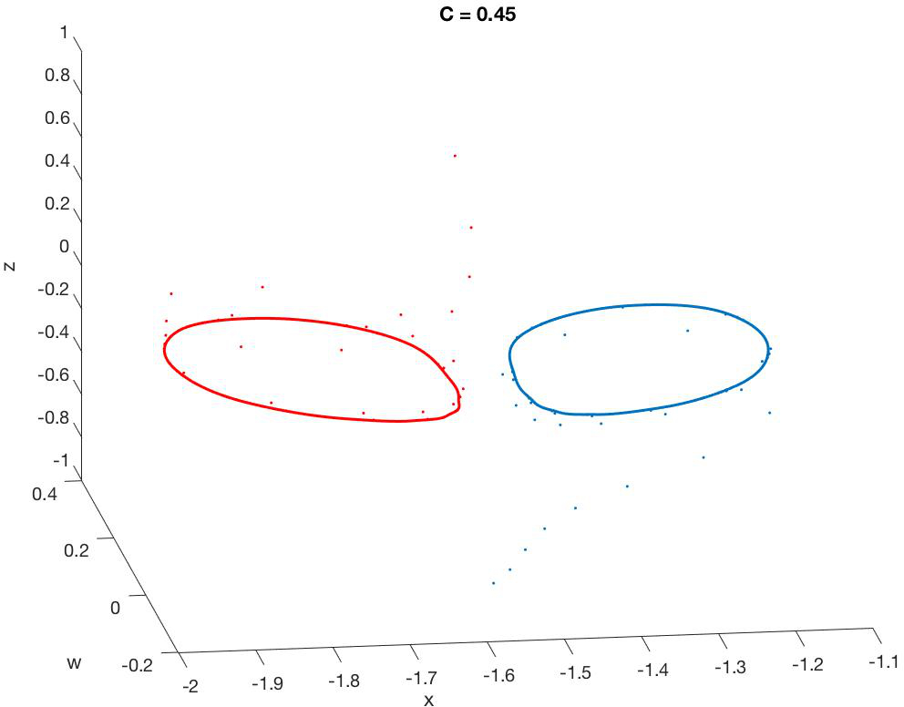
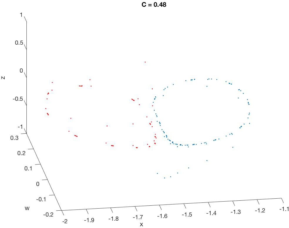
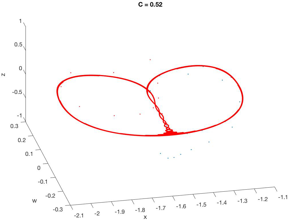
Figure 6: Bifurcation evolution for the map $E$ (5).

4.2 A more complex 3-dimensional generalization

We can create a more interesting extension of Gilet’s map by adding a dependence of the $z$-coordinate map on the other variables; for example, as in

$$\hat{E}(x,y,z;\sigma):=\left(x-\sigma\Psi^{\prime}(x)y,\mu(y+\Psi(x)),0.8z+0.1\sin^{2}(z+\Psi^{\prime}(x)\right).$$ (6)

It is easy to verify that the fixed points of (6) are as follows: There are, as for (5), denumerably many fixed points of the type $\left(x_{k},\mu(1-\mu)^{-1}\Psi(x_{k}),0\right)$, with $\Psi^{\prime}(x_{k})=0$, each having a 2-dimensional stable and 1-dimensional unstable manifold. There are also denumerably many fixed points of the form $\left(\tilde{x}_{m},0,z_{m}\right)$, with $\Psi(x_{m})=0$ and $z_{m}$ the unique solution of $2z_{m}=\sin^{2}\left(z_{m}+\Psi^{\prime}(x_{m})\right)$. These latter fixed points start as sinks and bifurcate into hyperbolic fixed points each with a 2-dimensional unstable manifold and a 1-dimensional stable manifold parallel to the $z$-axis. Moreover, the cylinders $C(\sigma)\times\mathbb{R}$ are attracting and invariant for sufficiently large values of the parameter $\sigma$. The main difference between this extension and (5) is that the unstable manifolds for the fixed points $\left(x_{k},\mu(1-\mu)^{-1}\Psi(x_{k}),0\right)$ do not remain in the $x,y$-plane as they wrap around the cylinder $C(\sigma)\times\mathbb{R}$, which leads to the more complex bifurcation behavior shown in Fig. 7.

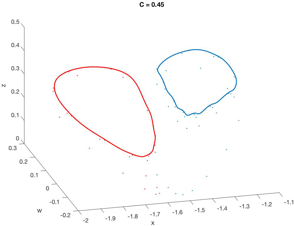
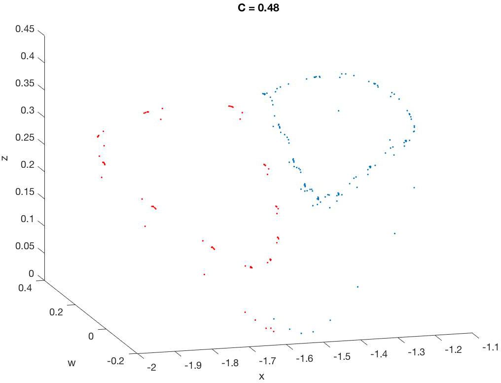
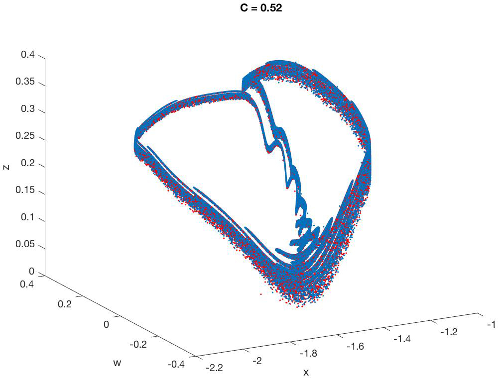
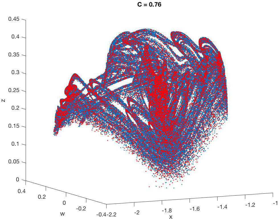
Figure 7: Bifurcation evolution for the map $\hat{E}$ (6).

5 Examples

Here we shall present examples of the bifurcation behavior described in Theorem 1 and Theorem 2, mainly through illustrations based on simulations and a bit of analysis. The examples, which comprise a homoclinic and heteroclinic-homoclinic type, are to be planar maps based upon Gilet’s model and a minor modification thereof.

5.1 Symmetric homoclinic bifurcations for Gilet’s map

It turns out that homoclinic bifurcations of the type described in Theorem 1 can be very effectively illustrated by considering a pair of contiguous symmetric cells (containing symmetric invariant closed curves with source point centers along the $x$-axis) for Gilet’s map

$$F(x,y;\sigma):=\left(x-\sigma\Psi^{\prime}(x)y,\mu(y+\Psi(x))\right),$$ (7)

where $\mu$ is fixed and $\sigma=C$ is varied. The symmetric cells are chosen to be the ones symmetric about the stable manifold corresponding to the line $x\simeq-1.57$, with symmetric center sources (approximately) at $\left(-1.79,0\right)$ and $\left(-1.35,0\right)$ as shown in Fig. 8. It should be noted that, in contrast to the description in Theorem 1, the saddle point on the stable manifold is below rather than above the symmetric invariant closed attracting curves, which means that the assumptions remain the same modulo a reflection in the $x$-axis.

Now, it is a straightforward but rather tedious matter to verify that all of the hypotheses of Theorem 1 hold (modulo the reflection mentioned above), but all of the assumptions are illustrated quite clearly in Fig. 8 save the existence of the orientation reversing slice regions. Consequently, we shall restrict our analysis to the identification of these regions for this example. A simple calculation shows that the saddle point of interest in this example is fixed at $\boldsymbol{p}=\left(\hat{x},\mu(1-\mu)^{-1}\Psi(\hat{x})\right)\simeq\left(-1.57,\mu(1-\mu)^{-1}\Psi(-1.57)\right)\simeq\left(-1.57,-0.206\mu(1-\mu)^{-1}\right).$ We also compute that

$$\det F^{\prime}=\mu\left[1-\sigma\left(y\Psi^{\prime\prime}(x)-(\Psi^{\prime}(x))^{2}\right)\right],$$

so it follows from the fact that $\Psi^{\prime\prime}(x)$ is positive $\left(\simeq\Psi^{\prime\prime}(\hat{x})\right)$ in a thin vertical strip centered at $x=\hat{x}$. Hence, it follows that $\det F^{\prime}$ changes from positive to negative along the stable manifold as $y$ changes from negative to positive, which signals a reversal of orientation.

The change in orientation also produces the slice regions $Z$ described in (A2). To see this, it follows from symmetry that it is enough to describe the slice to the right of the stable manifold $x=\hat{x}$. Of course, the left boundary curve for this slice is just a portion of the vertical line $x=\hat{x}$ for $y\geq\tilde{y}>0.$ The right-hand boundary curve for the slice is just

$$y=\frac{x-\hat{x}}{\sigma\Psi^{\prime}(x)}$$

for $x>\hat{x}$, which has a cusp at $\left(\hat{x},\tilde{y}\right)$, where

$$\tilde{y}=\lim_{x\downarrow\hat{x}}\left(\frac{x-\hat{x}}{\sigma\Psi^{\prime}(x)}\right).$$

Now it is straightforward to verify that this slice region has the properties described in (A2) and (A3) of Theorem1, as does the symmetric slice to the left of $x=\hat{x}.$

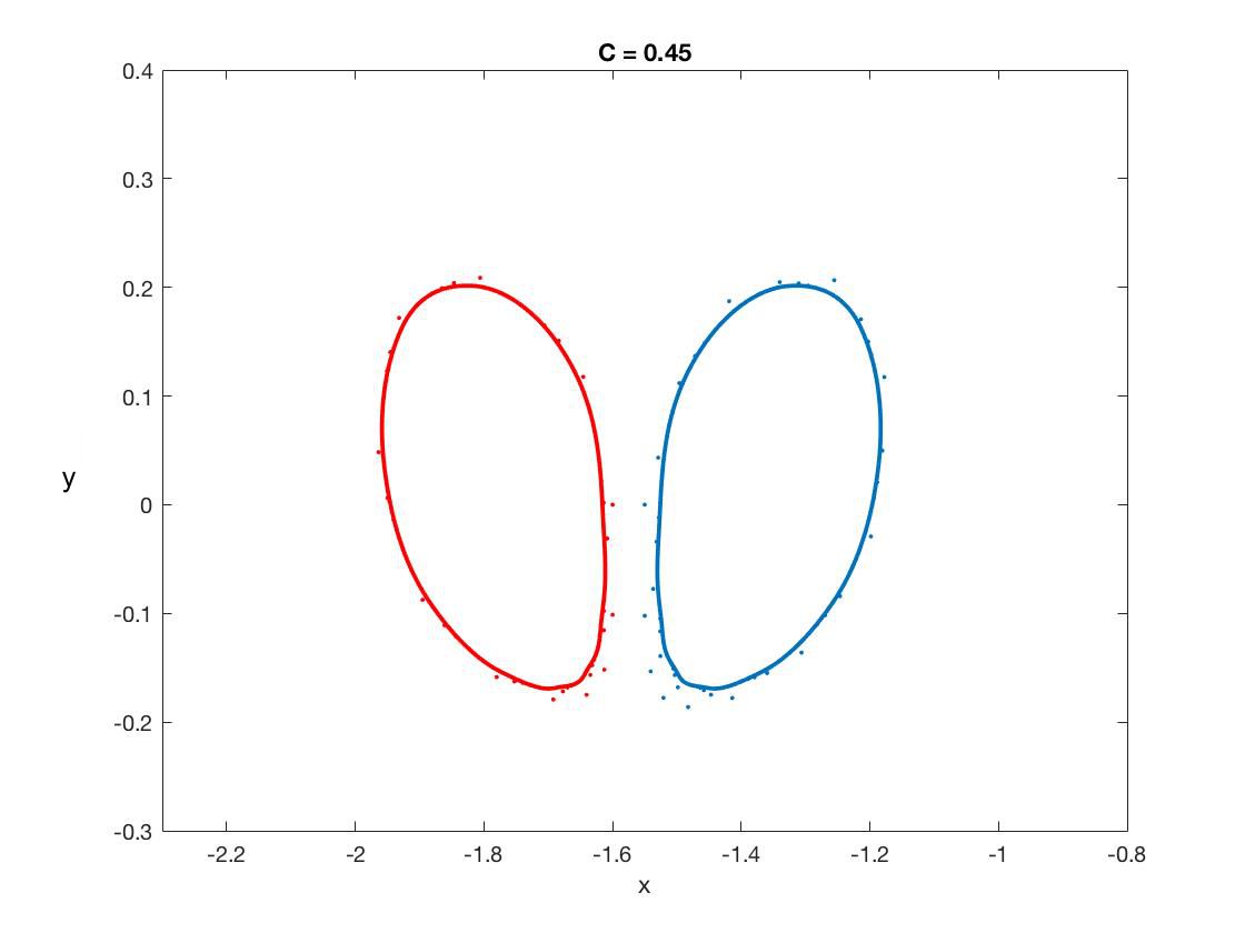
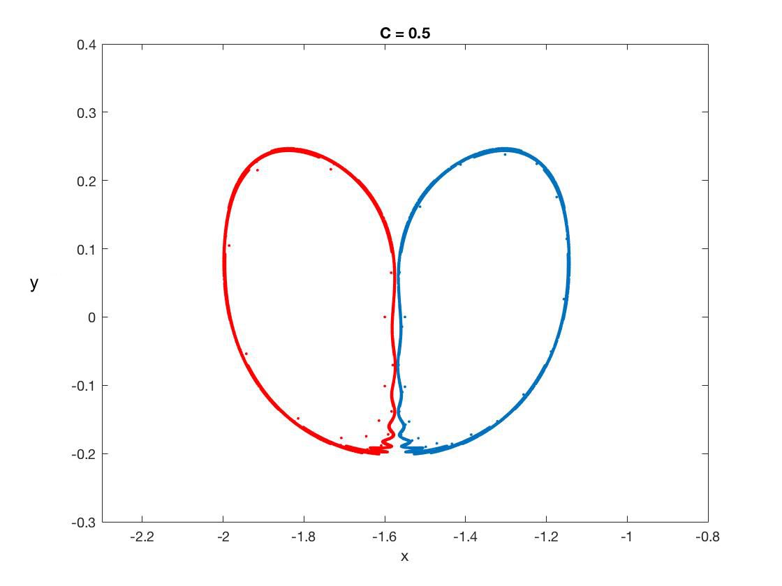
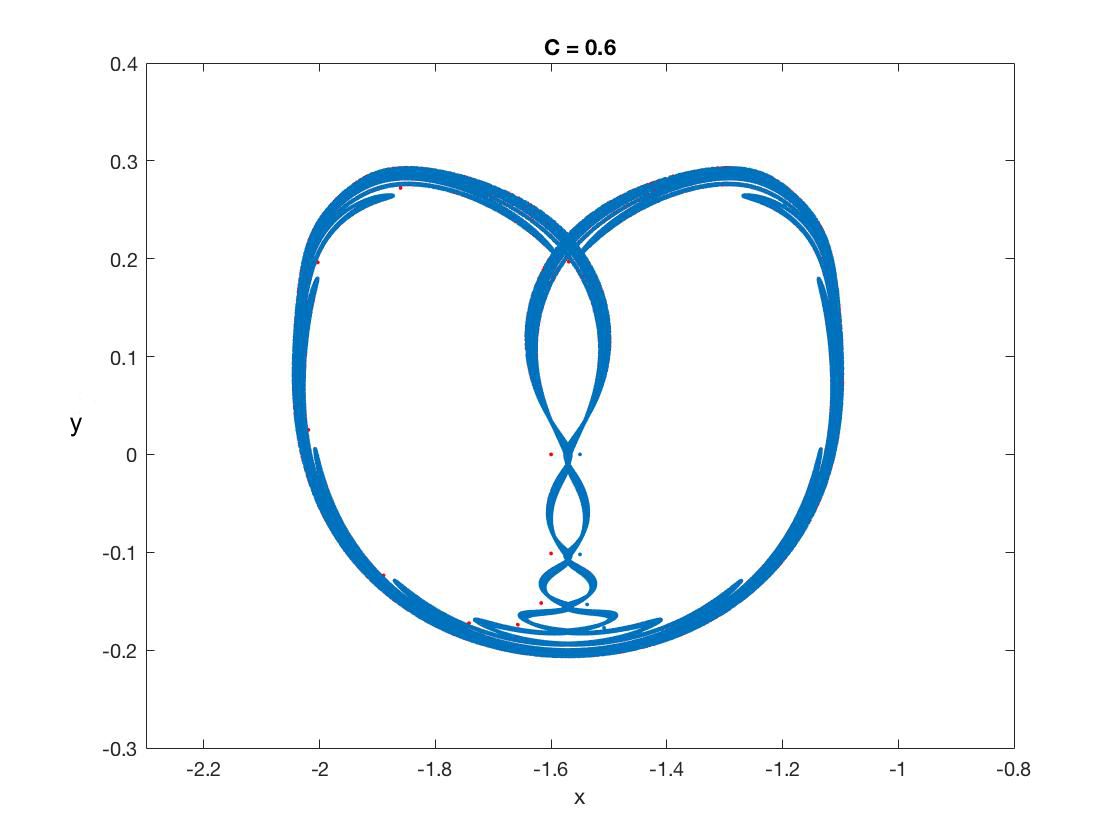
Figure 8: Bifurcation evolution for the map $F$ (7).

5.2 Heteroclinic-homoclinic bifurcations for modified Gilet’s map

To illustrate the bifurcations in Theorem 2, we consider the following modification of Gilet’s map: It is the map $\tilde{F}:\mathbb{R}^{2}\rightarrow\mathbb{R}^{2}$ defined as follows:

$$\tilde{F}(x,y;\sigma):=\left\{\begin{array}[c]{cc}F(x,y;\sigma),&\left|x\right|\leq 0.4\\ \left(x-[1+5(x+0.4)]\sigma\tilde{\Psi}^{\prime}(x)y,\mu(y+\tilde{\Psi}(x))\right),&-0.6<x<-0.4\\ \left(x-[1-5(x-0.4)]\sigma\tilde{\Psi}^{\prime}(x)y,\mu(y+\tilde{\Psi}(x))\right),&0.4<x<0.6\\ \left(x,\mu(y+\tilde{\Psi}(x))\right),&\left|x\right|\geq 0.6\end{array}\right.,$$ (8)

where

$$\tilde{\Psi}(x):=\left\{\begin{array}[c]{cc}\left(10x+3\right)\Psi(0.4),&-0.6<x<-0.4\\ (10x-3)\Psi(0.4),&0.4<x<0.6\\ -3\Psi(0.4),&x\leq-0.6\\ 3\Psi(0.4),&0.6\leq x\end{array}\right..$$

We note that the map (8) is continuous everywhere and smooth except along the lines $x=\pm 0.4,\pm 0.6$. It turns out that the vertical lines along which it fails to be $C^{\infty}$ do not alter the qualitative nature of the bifurcation evolution as described in Theorem 2, which is evident from Fig. 9. Once again, we note that the hypotheses of Theorem 2 can be readily checked, but all save the existence of the $Z$ slices are clearly shown in the simulations in Fig. 9. The existence of the orientation reversing slices $Z(\sigma)$ and $\breve{Z}(\sigma)$ can be verified in a manner completely analogous to to that used in the previous example.

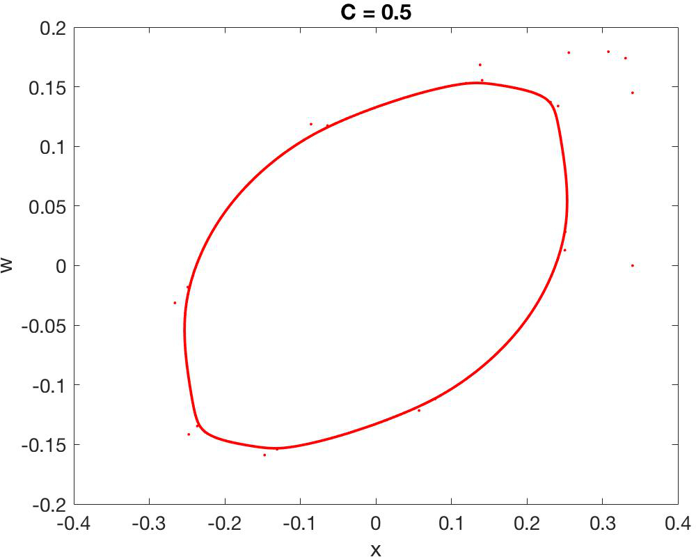
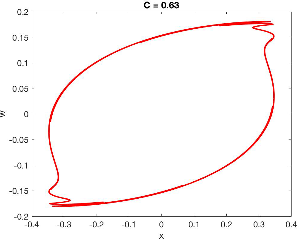
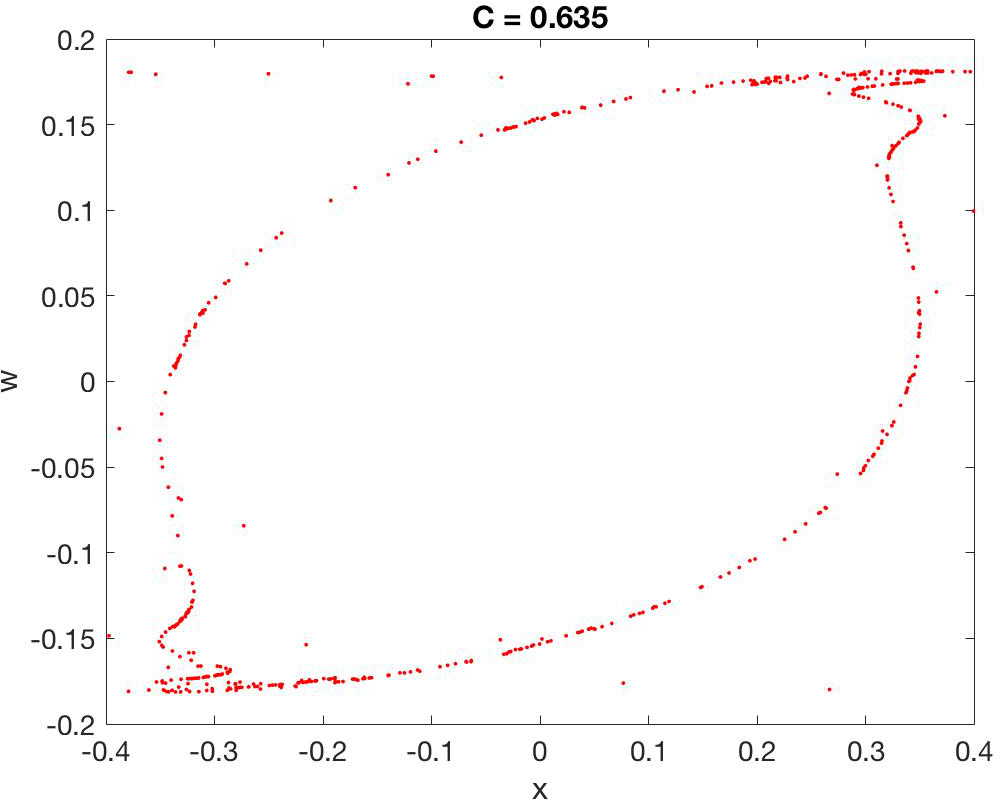
Figure 9: Bifurcation evolution for the map $\tilde{F}$ (8).

6 Concluding Remarks

In our paper [16], we proved that Gilet’s walking droplet model [7] develops Neimark–Sacker bifurcations generating invariant attracting closed Jordan curves (topological circles) as either one of the parameters is increased. We also saw that the diameter of these circles increases with either increasing parameter, which ultimately gives rise to new types of bifurcations arising from the interactions of stable manifolds with unstable manifolds of saddle points winding around the expanding circles. The investigation in this paper comprises an in-depth analysis of two variants - one purely homoclinic and the other a combination of heteroclinic and homoclinic interactions of unstable and stable manifolds of saddle points - of these new bifurcations as the original interaction parameter $C$ (identified with $\sigma$) is varied while the damping parameter $\mu$ is fixed. In addition to our analysis of these bifurcations, we showed by examples how these dynamical phenomena can be extended to higher dimensions.

There are several research directions related to this work that we intend to pursue in the near future. First among these is a related new bifurcation somewhat like those studied here, but based on diffeomorphisms that do not include the orientation reversing, noninjective slice regions in Gilet’s model. Naturally, we also intend to study the bifurcations in models of Gilet type with $C$ fixed and $\mu$ varying, which, for example, appears to exhibit more striking dynamical crises behavior than the case studied here. Another line of research, which has strong connections with the quantum aspects of pilot waves, is the construction of invariant or approximately invariant measures for the dynamical models such as Gilet’s and is something that we intend to investigate as part of our continuing investigation of the mathematical aspects of walking droplet phenomena.

References

- [1] D.G. Aronson, M.A. Chory, G.R Hall and R.P. McGehee, Bifurcations from an invariant circle for two-parameter families of maps of the plane: a computer-assisted study, Commun. Math. Phys. 83 (1982), 303-354.
- [2] D. K. Arrowsmith and C. M. Place, Dynamical Systems: Differential Equations, Maps and Chaotic Behaviour, Chapman and Hall, London, 1992.
- [3] A. Bertozzi, Heteroclinic orbits and chaotic dynamics in planar fluid flow, SIAM J. Math. Anal. 19 (1998), 1271-1294.
- [4] J. Bush, Pilot-wave hydrodynamics, Ann. Rev. Fluid Mech. 49 (2015), 269-292.
- [5] Y. Couder, S. Protiere, E. Fort, A. Boudaoud, Dynamical phenomena: Walking and orbiting droplets, Nature 437 (2005), 208.
- [6] C.E. Frouzakis, I.G. Kevrekidis and B.P. Peckham, A route to computational chaos revisited: noninvertibility and the breakup of an invariant circle, Physica D 177 (2003), 101-121.
- [7] T. Gilet, Dynamics and statistics of wave-particle interactions in a confined geometry, Phys. Rev. E 90 (2013), 05297.
- [8] Y. Joshi and D. Blackmore, Strange attractors for asymptotically zero maps, Chaos, Solitons & Fractals 68 (2014), 123-138.
- [9] P. Milewski, C. Galeano-Rios, A. Nachbin and J. Bush, Faraday pilot-wave dynamics: modeling and computation, J. Fluid Mech. 778 (2015), 361-388.
- [10] J. Moser, Stable and Random Motion in Dynamical Systems, Princeton University Press, Princeton, 1973.
- [11] J. Neimark, On some cases of periodic motions depending on parameters, Dokl. Akad. Nauk SSSR 129 (1959), 736-739.
- [12] S. Newhouse, Diffeomorphisms with infinitely many sinks, Topology 13 (1974), 9-18.
- [13] E. Ott, Chaos in Dynamical Systems, Cambridge University Press, Cambridge, 1993.
- [14] A. Oza, D. Harris, R. Rosales and J. Bush, Pilot-wave dynamics in a rotating frame: the emergence of orbital quantification, J. Fluid Mech. 744 (2014), 404-429.
- [15] J. Palis and W. de Melo, Geometric Theory of Dynamical Systems: An Introduction, Springer-Verlag, New York, 1982.
- [16] A. Rahman and D. Blackmore, Neimark–Sacker bifurcations and evidence of chaos in a discrete dynamical model of walkers, Chaos, Solitons & Fractals 91 (2016), 339-349.
- [17] C. Robinson, Dynamical Systems: Stability, Symbolic Dynamics, and Chaos, CRC Press Inc., Boca Raton, 1995.
- [18] R. Sacker, On invariant surfaces and bifurcation of periodic solutions of ordinary differential equations, Rep. IMM-NYU 333 (1964), 1-62.
- [19] D. Shirokov, Bouncing droplets on a billiard table, Chaos 23 (2013), 013115.
- [20] S. Smale, The Mathematics of Time: Essays on Dynamical Systems, Economic Processes, and Related Topics, Springer-Verlag, New York, 1980.
- [21] Q. Wang and L-S. Young, Strange attractors with one dimension of instability, Commun. Math. Phys. 218 (2001), 1-97.
- [22] Q. Wang and L-S. Young, From invariant curves to strange attractors, Commun. Math. Phys. 225 (2002), 275-304.
- [23] Q. Wang and L-S. Young, Toward a theory of rank one attractors, Ann. of Math. (2) 167 (2008), 349-480.
- [24] S. Wiggins, Introduction to Applied Nonlinear Dynamical Systems and Chaos, Springer, New York, 2003.