Bayesian Compressive Sensing Using Normal Product Priors

Zhou Zhou, Kaihui Liu, and Jun Fang Zhou Zhou, Kaihui Liu, and Jun Fang are with the National Key Laboratory on Communications, University of Electronic Science and Technology of China, Chengdu 611731, China, Email: ZhouZhou@std.uestc.edu.cn; kaihuil@std.uestc.edu.cn; JunFang@uestc.edu.cnThis work was supported in part by the National Science Foundation of China under Grant 61172114.
Abstract

In this paper, we introduce a new sparsity-promoting prior, namely, the “normal product” prior, and develop an efficient algorithm for sparse signal recovery under the Bayesian framework. The normal product distribution is the distribution of a product of two normally distributed variables with zero means and possibly different variances. Like other sparsity-encouraging distributions such as the Student’s t𝑡t-distribution, the normal product distribution has a sharp peak at origin, which makes it a suitable prior to encourage sparse solutions. A two-stage normal product-based hierarchical model is proposed. We resort to the variational Bayesian (VB) method to perform the inference. Simulations are conducted to illustrate the effectiveness of our proposed algorithm as compared with other state-of-the-art compressed sensing algorithms.

Index Terms:
Compressed Sensing, sparse Bayesian learning, normal product prior.

I Introduction

Compressed sensing [1, 2] is a new data acquisition technique that has attracted much attention over the past decade. Existing methods for compressed sensing can generally be classified into the following categories, i.e. the greedy pursuit approach [3], the convex relaxation-type approach [4] and the nonconvex optimization method [5]. Another class of compressed sensing techniques that have received increasing attention are Bayesian methods. In the Bayesian framework, the signal is usually assigned a sparsity-encouraging prior, such as the Laplace prior and the Gaussian-inverse Gamma prior [6], to encourage sparse solutions. It has been shown in a series of experiments that Bayesian compressed sensing techniques [7] demonstrate superiority for sparse signal recovery as compared with the greedy methods and the basis pursuit method. One of the most popular prior model for Bayesian compressed sensing is the Gaussian-inverse Gamma prior proposed in [6]. The Gaussian-inverse Gamma prior is a two-layer hierarchical model in which the first layer specifies a Gaussian prior to the sparse signal and an inverse Gamma priori is assigned to the parameters characterizing the Gaussian prior. As discussed in [8], this two-stage hierarchical model is equivalent to imposing a Student’s t𝑡t-distribution on the sparse signal. Besides the Gaussian-inverse Gamma prior, authors in [9] employ Laplace priors for the sparse signal to promote sparse solutions.

In this paper, we introduce a new sparsity-encouraging prior, namely, the normal product (NP) prior, for sparse signal recovery. A two-stage normal product-based hierarchical model is established, and we resort to the variational Bayesian (VB) method to perform the inference for the hierarchical model. Our experiments show that the proposed algorithm achieves similar performance as the sparse Bayesian learning method, while with less computational complexity.

II The Bayesian Network
Refer to caption
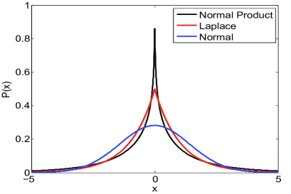
Figure 1: Three kinds of PDF with the same standard deviation

In the context of compressed sensing, we are given a noise corrupted linear measurements of a vector 𝐱0subscript𝐱0{\bf{x}}_{0}

𝐲=𝐀𝐱0+𝐧𝐲subscript𝐀𝐱0𝐧{\bf{y}}={\bf{A}}{{\bf{x}}_{{0}}}+{\bf{n}} (1)

Here 𝐀𝐑M×N𝐀superscript𝐑𝑀𝑁{\bf{A}}\in{{\bf{R}}^{M\times N}} is an underdetermined measurement matrix with low coherence of columns, 𝐧𝐑M𝐧superscript𝐑𝑀{\bf{n}}\in{{\bf{R}}^{M}} represents the acquisition noise vector and 𝐱0subscript𝐱0{\bf x}_{0} a sparse signal. For the inverse problem, both 𝐱0subscript𝐱0{\bf x}_{0} and 𝐧𝐧\bf n are unknown, and our goal is to recover 𝐱0subscript𝐱0{\bf x}_{0} from 𝐲𝐲\bf y. We formulate the observation noise as zero mean independent Gaussian variable with variance ξ2superscript𝜉2{\xi^{2}} i.e. 𝐲N(𝐀𝐱0,ξ2𝐈)similar-to𝐲𝑁subscript𝐀𝐱0superscript𝜉2𝐈{\bf{y}}\sim N({{\bf{A}}{{{\bf x}_{0}}}},{\xi^{2}}\bf{I}) and seek a sparse signal 𝐱=Δ(x1,x2,xN)superscriptΔ𝐱subscript𝑥1subscript𝑥2subscript𝑥𝑁{\bf x}\buildrel\Delta\over{=}({x_{1}},{x_{2}},\ldots{x_{N}}) for 𝐱0subscript𝐱0{\bf x}_{0}.

In this section, we utilize a two-stage hierarchical bayesian prior for the signal model. In the first layer of signal model, we use the Normal Product (NP) distribution as sparseness prior:

𝐱NP(𝟎,𝚺)similar-to𝐱𝑁𝑃0𝚺{\bf{x}}\sim NP({\bf{0}},{\bf{\Sigma}})

where 𝟎𝐑N0superscript𝐑𝑁{\bf{0}}\in{{\bf{R}}^{N}} stands for its mean and 𝚺𝚺{\bf{\Sigma}} given as a diagonal matrix diag(σ12,σ22,,σN2)𝐑N×Ndiagsuperscriptsubscript𝜎12superscriptsubscript𝜎22superscriptsubscript𝜎𝑁2superscript𝐑𝑁𝑁{\text{diag}}({\sigma_{1}}^{2},{\sigma_{2}}^{2},\ldots,{\sigma_{N}}^{2})\in{{\bf{R}}^{N\times N}} represents its variance. For each element xisubscript𝑥𝑖{x_{i}} of 𝐱𝐱{\bf{x}} , its probability density distribution is K0(|xi|σi)/πσisubscript𝐾0subscript𝑥𝑖subscript𝜎𝑖/𝜋subscript𝜎𝑖{{{K_{0}}\left({\frac{{|{x_{i}}|}}{{{\sigma_{i}}}}}\right)}\mathord{\left/{\vphantom{{{K_{0}}\left({\frac{{|{x_{i}}|}}{{{\sigma_{i}}}}}\right)}{\pi{\sigma_{i}}}}}\right.\kern-1.2pt}{\pi{\sigma_{i}}}}, which exhibits a sharp peak at the origin and heavy tails, where K0()subscript𝐾0{K_{0}}(\cdot) is the zero order modified Bessel function of the second kind[10] thus the probability density function (PDF) of 𝐱𝐱\bf x is

1πNi=1N1σiK0(|xi|σi).1superscript𝜋𝑁superscriptsubscriptproduct𝑖1𝑁1subscript𝜎𝑖subscript𝐾0subscript𝑥𝑖subscript𝜎𝑖\frac{1}{{{\pi^{N}}}}\prod\nolimits_{i=1}^{N}{\frac{1}{{{\sigma_{i}}}}{K_{0}}(\frac{{\left|{{x_{i}}}\right|}}{{{\sigma_{i}}}})}. (2)

A NP distributed scaler variate xi𝐑subscript𝑥𝑖𝐑x_{i}\in{\bf{R}} can be decomposed as the product of two independent normally distributed variables i.e. if xiNP(0,σi2)similar-tosubscript𝑥𝑖𝑁𝑃0superscriptsubscript𝜎𝑖2x_{i}\sim NP(0,\sigma_{i}^{2}), then there are aiN(0,κi2)similar-tosubscript𝑎𝑖𝑁0superscriptsubscript𝜅𝑖2a_{i}\sim N(0,\kappa_{i}^{2}) and biN(0,γi2)similar-tosubscript𝑏𝑖𝑁0superscriptsubscript𝛾𝑖2b_{i}\sim N(0,\gamma_{i}^{2}) satisfying xi=aibisubscript𝑥𝑖subscript𝑎𝑖subscript𝑏𝑖x_{i}=a_{i}b_{i} with moment relationship σi=γiκisubscript𝜎𝑖subscript𝛾𝑖subscript𝜅𝑖\sigma_{i}=\gamma_{i}\kappa_{i}[11]. We call this property as the generating rule of Normal Product distribution. Similarly for the vector 𝐱𝐱{\bf{x}}, we can decompose it into the Hadamard product of two independent virtual normally distributed vector variables 𝐚𝐚{\bf{a}} and 𝐛𝐛{\bf{b}} whose variance are diagonal matrix 𝜿2=Δdiag(κ12,κ22,,κN2)superscriptΔsuperscript𝜿2diagsuperscriptsubscript𝜅12superscriptsubscript𝜅22superscriptsubscript𝜅𝑁2{{\boldsymbol{\kappa}}^{2}}\buildrel\Delta\over{=}{\text{diag}}(\kappa_{1}^{2},\kappa_{2}^{2},\ldots,\kappa_{N}^{2}) and 𝜸2=Δdiag(γ12,γ22,,γN2)superscriptΔsuperscript𝜸2diagsuperscriptsubscript𝛾12superscriptsubscript𝛾22superscriptsubscript𝛾𝑁2{{\boldsymbol{\gamma}}^{2}}\buildrel\Delta\over{=}{\text{diag}}(\gamma_{1}^{2},\gamma_{2}^{2},\ldots,\gamma_{N}^{2}) respectively i.e. 𝒙=𝒂𝒃𝒙𝒂𝒃{\boldsymbol{x}}={{\boldsymbol{a}}}\circ{{\boldsymbol{b}}} and 𝚺=𝜿2𝜸2𝚺superscript𝜿2superscript𝜸2{\boldsymbol{\Sigma}}={{\boldsymbol{\kappa}}^{2}}\circ{{\boldsymbol{\gamma}}^{2}}, where \circ denote the Hadamard product. Finally, we set σi2superscriptsubscript𝜎𝑖2\sigma_{i}^{-2} as a realization of Gamma hyperprior Γ(α,β)Γ𝛼𝛽\Gamma(\alpha,\beta) and choose α0𝛼0\alpha\to 0,β0𝛽0\beta\to 0 to construct a sharper distribution of 𝐱𝐱{\bf{x}} during the variational procedure [12] for the second layer of signal.

According to the generating rule of Normal Product mentioned above, we can add two parallel nodes 𝐚𝐚{\bf{a}} and 𝐛𝐛{\bf{b}} to construct one latent layer. Then the posterior distribution can be expressed as:

P𝐱(𝐱,𝚺|𝐲;α,β)=P(𝐱,𝐚,𝐛,𝚺|𝐲;α,β)𝑑𝐚𝑑𝐛subscript𝑃𝐱𝐱conditional𝚺𝐲𝛼𝛽𝑃𝐱𝐚𝐛conditional𝚺𝐲𝛼𝛽differential-d𝐚differential-d𝐛{P_{\bf{x}}}({\bf{x}},{\bf{\Sigma}}|{\bf{y}};\alpha,\beta)=\int{P({\bf{x}},{\bf{a}},{\bf{b}},{\bf{\Sigma}}|{\bf{y}};\alpha,\beta)d{\bf{a}}d{\bf{b}}}

where

P(𝐱,𝐚,𝐛,𝚺|𝐲;α,β)P(𝐲|𝐱)P(𝐱|𝐚,𝐛)P(𝐚|κ2)P(𝐛|γ2)P(𝚺|α,β)=P(𝐲𝐀𝐱)δ(𝐱𝐚𝐛)P(𝐚|κ2)P(𝐛|γ2)P(𝚺|α,β)𝑃𝐱𝐚𝐛conditional𝚺𝐲𝛼𝛽proportional-toabsent𝑃conditional𝐲𝐱𝑃conditional𝐱𝐚𝐛𝑃conditional𝐚superscript𝜅2𝑃conditional𝐛superscript𝛾2𝑃conditional𝚺𝛼𝛽absent𝑃𝐲𝐀𝐱𝛿𝐱𝐚𝐛𝑃conditional𝐚superscript𝜅2𝑃conditional𝐛superscript𝛾2𝑃conditional𝚺𝛼𝛽\begin{array}[]{l}P({\bf{x}},{\bf{a}},{\bf{b}},{\bf{\Sigma}}|{\bf{y}};\alpha,\beta)\\ \propto P({\bf{y}}|{\bf{x}})P({\bf{x}}|{\bf{a}},{\bf{b}})P({\bf{a}}|{{\bf{\kappa}}^{2}})P({\bf{b}}|{{\bf{\gamma}}^{2}})P({\bf{\Sigma}}|\alpha,\beta)\\ =P({\bf{y}}-{\bf{Ax}})\delta({\bf{x}}-{\bf{a}}\circ{\bf{b}})P({\bf{a}}|{{\bf{\kappa}}^{2}})P({\bf{b}}|{{\bf{\gamma}}^{2}})P({\bf{\Sigma}}|\alpha,\beta)\end{array}

and δ()𝛿\delta(\cdot) denotes the Dirac Delta function. In this expression we know that the value of 𝐱𝐱{\bf{x}} must be equal to 𝐚𝐛𝐚𝐛{\bf{a}}\circ{\bf{b}} while keeping the value of P(𝐱,𝐚,𝐛,𝚺|𝐲;α,β)𝑃𝐱𝐚𝐛conditional𝚺𝐲𝛼𝛽P({\bf{x}},{\bf{a}},{\bf{b}},{\bf{\Sigma}}|{\bf{y}};\alpha,\beta) nonzero. Consider the Bayesian Risk function:

E(L(𝐱^,𝐱))=L(𝐱^,𝐱)P𝐱(𝐱,𝚺|𝐲;α,β)𝑑𝐱𝑑𝚺L(𝐱^,𝐚𝐛)P𝐚,𝐛(𝐚,𝐛,𝚺|𝐲;α,β)𝑑𝐚𝑑𝐛𝑑𝚺𝐸𝐿^𝐱𝐱𝐿^𝐱𝐱subscript𝑃𝐱𝐱conditional𝚺𝐲𝛼𝛽differential-d𝐱differential-d𝚺proportional-toabsent𝐿^𝐱𝐚𝐛subscript𝑃𝐚𝐛𝐚𝐛conditional𝚺𝐲𝛼𝛽differential-d𝐚differential-d𝐛differential-d𝚺\begin{array}[]{l}E(L({\bf{\hat{x}}},{\bf{x}}))=\int{L({\bf{\hat{x}}},{\bf{x}})}{P_{\bf{x}}}({\bf{x}},{\bf{\Sigma}}|{\bf{y}};\alpha,\beta)d{\bf{x}}d{\bf{\Sigma}}\\ \propto\int{L({\bf{\hat{x}}},{\bf{a}}\circ{\bf{b}})}{P_{{\bf{a}},{\bf{b}}}}({\bf{a}},{\bf{b}},{\bf{\Sigma}}|{\bf{y}};\alpha,\beta)d{\bf{a}}d{\bf{b}}d{\bf{\Sigma}}\end{array}

where

P𝐚,𝐛(𝐚,𝐛,𝚺|𝐲;α,β)=P(𝐲𝐀(𝐚𝐛))P(𝐚|𝜿2)P(𝐛|𝜸2)P(𝚺|α,β)subscript𝑃𝐚𝐛𝐚𝐛conditional𝚺𝐲𝛼𝛽absent𝑃𝐲𝐀𝐚𝐛𝑃conditional𝐚superscript𝜿2𝑃conditional𝐛superscript𝜸2𝑃conditional𝚺𝛼𝛽\begin{array}[]{l}{P_{{\bf{a}},{\bf{b}}}}({\bf{a}},{\bf{b}},{\bf{\Sigma}}|{\bf{y}};\alpha,\beta)\\ =P({\bf{y}}-{\bf{A}}({\bf{a}}\circ{\bf{b}}))P({\bf{a}}|{{\boldsymbol{\kappa}}^{2}})P({\bf{b}}|{{\boldsymbol{\gamma}}^{2}})P({\bf{\Sigma}}|\alpha,\beta)\end{array}

and L(𝐱^,𝐱)𝐿^𝐱𝐱L({\bf{\hat{x}}},{\bf{x}}) represents the loss function. Thus, we can replace P𝐱(𝐱,𝚺|𝐲;α,β)subscript𝑃𝐱𝐱conditional𝚺𝐲𝛼𝛽{P_{\bf{x}}}({\bf{x}},{\bf{\Sigma}}|{\bf{y}};\alpha,\beta) with P𝐚,𝐛(𝐚,𝐛,𝚺|𝐲;α,β)subscript𝑃𝐚𝐛𝐚𝐛conditional𝚺𝐲𝛼𝛽{P_{{\bf{a}},{\bf{b}}}}({\bf{a}},{\bf{b}},{\bf{\Sigma}}|{\bf{y}};\alpha,\beta) in the inference procedure while maintaining the value of the Bayesian risk function at a consistent level. So the modified Bayesian Network is:
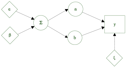
𝐲N(𝐀(𝐚𝐛),ξ2𝐈)similar-to𝐲𝑁𝐀𝐚𝐛superscript𝜉2𝐈{\bf{y}}\sim N({\bf{A}}({\bf{a}}\circ{\bf{b}}),{\xi^{2}}{\bf{I}}) (3)
𝐚N(𝟎,𝜿2)similar-to𝐚𝑁0superscript𝜿2{\bf{a}}\sim N({\bf{0}},{{\boldsymbol{\kappa}}^{2}}) (4)
𝐛N(𝟎,𝜸2)similar-to𝐛𝑁0superscript𝜸2{\bf{b}}\sim N({\bf{0}},{{\boldsymbol{\gamma}}^{2}}) (5)
σi2=γi2κi2Γ(α,β)superscriptsubscript𝜎𝑖2superscriptsubscript𝛾𝑖2superscriptsubscript𝜅𝑖2similar-toΓ𝛼𝛽\sigma_{i}^{-2}=\gamma_{i}^{-2}\kappa_{i}^{-2}\sim\Gamma(\alpha,\beta) (6)

as depicted in Fig. 2.

Refer to caption
Figure 2: The Bayesian Network

III The Varational Bayesian inference

In order to infer the bayesian network, we use the mean-field variational Bayesian method to analytically approximate the entire posterior distribution of latent variable. In this theorem, it was assumed that the approximate variational distribution q(𝐳|𝐲)𝑞conditional𝐳𝐲q({\bf{z}}|{\bf{y}}) where 𝐳𝐳\bf z stands for the latent variable in the model could be factorized into the product i=1lqi(𝐳i|𝐲)superscriptsubscriptproduct𝑖1𝑙subscript𝑞𝑖conditionalsubscript𝐳𝑖𝐲\prod\nolimits_{i=1}^{l}{{q_{i}}({{\bf{z}}_{i}}|{\bf{y}})} for the partition 𝐳1,,𝐳lsubscript𝐳1subscript𝐳𝑙{{\bf{z}}_{1}},\ldots,{{\bf{z}}_{l}} of 𝐳𝐳{\bf{z}}. It could be shown that the solution of the variational method for each factor qi(𝐳i|𝐲)subscript𝑞𝑖conditionalsubscript𝐳𝑖𝐲{q_{i}}({{\bf{z}}_{i}}|{\bf{y}}) could be written as:

qi(𝐳i|𝐲)=e<lnp(𝐳|𝐲))>𝐳ie<lnp(𝐳|𝐲))>𝐳i𝑑𝐳i{q_{i}}^{*}({{\bf{z}}_{i}}|{\bf{y}})=\frac{{{e^{<\ln p({\bf{z}}|{\bf{y}})){>_{\neq{{\bf{z}}_{i}}}}}}}}{{\int{{e^{<\ln p({\bf{z}}|{\bf{y}})){>_{\neq{{\bf{z}}_{i}}}}}}d{{\bf{z}}_{i}}}}}

where <lnp(𝐳|𝐲))>𝐳i<\ln p({\bf{z}}|{\bf{y}})){>_{\neq{{\bf{z}}_{i}}}} means taking the expectation over the set of 𝐳𝐳{\bf{z}} using the variational distribution except 𝐳isubscript𝐳𝑖{{\bf{z}}_{i}}[13] . Applying the variational Bayesian method upon the bayesian model mentioned in secetion II, the posterior approximation of 𝚺,𝐚,𝐛𝚺𝐚𝐛{\bf{\Sigma}},{\bf{a}},{\bf{b}} are respectively:

ln(q(𝐚))<lnP(𝐚,𝐛,𝚺|𝐲;α,β)>q(𝐛),q(𝚺)\ln({q^{*}}({\bf{a}}))\propto<\ln P({\bf{a}},{\bf{b}},{\bf{\Sigma}}|{\bf{y}};{\bf{\alpha}},{\bf{\beta}}){>_{{q^{*}}({\bf{b}}),{q^{*}}({\bf{\Sigma}})}} (7)
ln(q(𝐛))<lnP(𝐚,𝐛,𝚺|𝐲;α,β)>q(𝐚),q(𝚺)\ln({q^{*}}({\bf{b}}))\propto<\ln P({\bf{a}},{\bf{b}},{\bf{\Sigma}}|{\bf{y}};{\bf{\alpha}},{\bf{\beta}}){>_{{q^{*}}({\bf{a}}),{q^{*}}({\bf{\Sigma}})}} (8)
ln(q(𝚺))<lnP(𝐚,𝐛,𝚺|𝐲;α,β)>q(𝐛),q(𝐚)\ln({q^{*}}({\bf{\Sigma}}))\propto<\ln P({\bf{a}},{\bf{b}},{\bf{\Sigma}}|{\bf{y}};{\bf{\alpha}},{\bf{\beta}}){>_{{q^{*}}({\bf{b}}),{q^{*}}({\bf{a}})}} (9)

III-A posterior approximation of 𝐚𝐚{\bf{a}} and 𝐛𝐛{\bf{b}}

Substituting (3), (4), (5) and (6) into (8), we can arrive at:

q(𝐛)N(𝚪1𝐜,𝚪1)similar-tosuperscript𝑞𝐛𝑁superscriptsuperscript𝚪1superscript𝐜superscriptsuperscript𝚪1{q^{*}}({\bf{b}}){\sim}\;N({{\bf{\Gamma}}^{\prime}}^{-1}{{\bf{c}}^{\prime}},{{\bf{\Gamma}}^{\prime}}^{-1})

where

𝚪=1ξ2(𝐀T𝐀)<𝐚𝐚T>q(𝐚)+<𝜸2>q(𝜸)superscript𝚪1superscript𝜉2superscript𝐀𝑇𝐀subscriptexpectationsuperscript𝐚𝐚𝑇superscript𝑞𝐚subscriptexpectationsuperscript𝜸2superscript𝑞𝜸{{\bf{\Gamma}}^{\prime}}=\frac{1}{{{\xi^{2}}}}({{\bf{A}}^{T}}{\bf{A}})\circ<{\bf{a}}{{\bf{a}}^{T}}{>_{{q^{*}}({\bf{a}})}}+<{{\boldsymbol{\gamma}}^{-2}}{>_{{q^{*}}({\boldsymbol{\gamma}})}}

and

𝐜=1ξ2diag(<𝐚>q(𝐚))𝐀T𝒚superscript𝐜1superscript𝜉2diagsubscriptexpectation𝐚superscript𝑞𝐚superscript𝐀𝑇𝒚{{\bf{c}}^{\prime}}=\frac{1}{{{\xi^{2}}}}{\text{diag}}\left({<{\bf{a}}{>_{{q^{*}}({\bf{a}})}}}\right){{\bf{A}}^{T}}\boldsymbol{y}

. From the principle of variational inference, we know that q(𝒃)𝑞𝒃q\left({\boldsymbol{b}}\right) is an approximation of P(𝒃|𝒚)𝑃conditional𝒃𝒚P(\boldsymbol{b}|\boldsymbol{y}) i.e. P(𝒃|𝒚)q(𝐛)𝑃conditional𝒃𝒚𝑞𝐛P(\boldsymbol{b}|\boldsymbol{y})\approx q\left({\bf{b}}\right) and in order to get a more concise iteration formula, we choose the relaxation of the secondary moment as:

<𝐚𝐚T>q(a)<𝐚>q(a)<𝐚T>q(a)subscriptexpectationsuperscript𝐚𝐚𝑇superscript𝑞𝑎subscriptexpectation𝐚superscript𝑞absent𝑎subscriptexpectationsuperscript𝐚𝑇superscript𝑞absent𝑎<{\bf{a}}{{\bf{a}}^{T}}{>_{{q^{*}}(a)}}\approx<{\bf{a}}{>_{{q^{**}}(a)}}<{{\bf{a}}^{T}}{>_{{q^{**}}(a)}}
<𝜸2>q(𝜸)<𝜸>q(𝜸)2subscriptexpectationsuperscript𝜸2superscript𝑞𝜸superscriptsubscriptexpectation𝜸superscript𝑞absent𝜸2<{{\boldsymbol{\gamma}}^{-2}}{>_{{q^{*}}({\boldsymbol{\gamma}})}}\approx<{\boldsymbol{\gamma}}>_{{q^{**}}({\boldsymbol{\gamma}})}^{-2}

This relaxation can be interpreted as ignoring the posteriori variance during the updating, which is inspired by the fact that after the learning procedure the posteriori variance always approaches zero to ensure the posteriori mean’s concentration on the estimated value.

Then the corrected posterior approximation is q(𝐛)N(𝚪1𝐜,𝚪1)similar-tosuperscript𝑞absent𝐛𝑁superscript𝚪1𝐜superscript𝚪1{q^{**}}({\bf{b}})\sim N({{\boldsymbol{\Gamma}}^{-1}}{\bf{c}},{{\boldsymbol{\Gamma}}^{-1}}) where

𝚪1={1ξ2(𝐀diag(<𝐚>q(𝐚)))T𝐀diag(<𝐚>q(𝐚))+<𝜸>q(𝜸)2}1\begin{array}[]{*{20}{l}}{{{\boldsymbol{\Gamma}}^{-1}}=\{\frac{1}{{{\xi^{2}}}}{{\left({{\bf{A}}{\rm{diag}}\left({<{\bf{a}}{>_{{q^{**}}({\bf{a}})}}}\right)}\right)}^{T}}{\bf{A}}{\rm{diag}}\left({<{\bf{a}}{>_{{q^{**}}({\bf{a}})}}}\right)}\\ {{\rm{+}}<{\boldsymbol{\gamma}}{>_{{q^{**}}({\boldsymbol{\gamma}})}}^{-2}{\}^{-1}}}\end{array}

and

𝐜=1ξ2diag(<𝐚>q(𝐚))𝐀T𝐲𝐜1superscript𝜉2diagsubscriptexpectation𝐚superscript𝑞absent𝐚superscript𝐀𝑇𝐲{{\bf{c}}=\frac{1}{{{\xi^{2}}}}{\rm{diag}}\left({<{\bf{a}}{>_{{q^{**}}({\bf{a}})}}}\right){{\bf{A}}^{T}}{\bf{y}}}

In the noise free case, using Woodbury identity we have:

limξ0𝚪1𝐜=<𝜸>q(𝜸)(𝐀diag(<𝐚>q(𝐚))<𝜸>q(𝜸))+𝐲subscript𝜉0superscript𝚪1𝐜missing-subexpressionmissing-subexpressionmissing-subexpressionmissing-subexpressionmissing-subexpressionmissing-subexpressionmissing-subexpressionmissing-subexpressionmissing-subexpressionmissing-subexpressionmissing-subexpressionmissing-subexpressionmissing-subexpressionmissing-subexpressionmissing-subexpressionmissing-subexpressionmissing-subexpressionmissing-subexpressionmissing-subexpressionabsentsubscriptexpectation𝜸superscript𝑞absent𝜸superscript𝐀diagsubscriptexpectation𝐚superscript𝑞absent𝐚subscriptexpectation𝜸superscript𝑞absent𝜸𝐲missing-subexpressionmissing-subexpressionmissing-subexpressionmissing-subexpressionmissing-subexpressionmissing-subexpressionmissing-subexpressionmissing-subexpressionmissing-subexpressionmissing-subexpressionmissing-subexpressionmissing-subexpressionmissing-subexpressionmissing-subexpressionmissing-subexpressionmissing-subexpressionmissing-subexpressionmissing-subexpressionmissing-subexpression\begin{array}[]{*{20}{l}}{\mathop{\lim}\limits_{\xi\to 0}{{\boldsymbol{\Gamma}}^{-1}}{\bf{c}}}\\ {=<{\boldsymbol{\gamma}}{>_{{q^{**}}({\boldsymbol{\gamma}})}}{{({\bf{A}}{\rm{diag}}(<{\bf{a}}{>_{{q^{**}}({\bf{a}})}})<{\boldsymbol{\gamma}}{>_{{q^{**}}({\boldsymbol{\gamma}})}})}^{+}}{\bf{y}}}\end{array} (10)

and

limξ0𝚪1=(𝐈<𝜸>𝐪(𝜸)(𝐀diag(<𝐛>𝐪(𝐛))<𝜸>𝐪(𝜸))+)×𝐀diag(<𝐚>q(𝐚))<𝜸>q(𝜸)2subscript𝜉0superscript𝚪1absent𝐈subscriptexpectation𝜸superscript𝐪absent𝜸superscript𝐀diagsubscriptexpectation𝐛superscript𝐪absent𝐛subscriptexpectation𝜸superscript𝐪absent𝜸absent𝐀diagsubscriptexpectation𝐚superscript𝑞absent𝐚superscriptsubscriptexpectation𝜸superscript𝑞absent𝜸2\begin{array}[]{l}{\lim_{\xi\to 0}}{{\bf{\Gamma}}^{-1}}\\ =(\bf{I}-<{\boldsymbol{\gamma}}{>_{{q^{**}}({\boldsymbol{\gamma}})}}{\left({{\bf{A}}{\text{diag}}\left({<{\bf{b}}{>_{{q^{**}}({\bf{b}})}}}\right)<{\boldsymbol{\gamma}}{>_{{q^{**}}({\boldsymbol{\gamma}})}}}\right)^{+}})\\ \times{\bf{A}}{\text{diag}}\left({<{\bf{a}}{>_{{q^{**}}({\bf{a}})}}}\right)<{\boldsymbol{\gamma}}>_{{q^{**}}({\boldsymbol{\gamma}})}^{2}\end{array} (11)

Similarly, for 𝐚𝐚{\bf{a}}, substituting (3), (4), (5) and (6) into (7), we have:

q(𝐚)N(𝐇1𝐟,𝐇1)similar-tosuperscript𝑞𝐚𝑁superscriptsuperscript𝐇1superscript𝐟superscriptsuperscript𝐇1{q^{*}}({\bf{a}}){\sim}\;N({{\bf{{H}}}^{\prime}}^{-1}{{\bf{f}}^{\prime}},{{\bf{{H}}}^{\prime}}^{-1})

where

𝐇=1ξ2(𝐀T𝐀)<𝐛𝐛T>q(𝐛)+<𝜿2>q(𝜿)superscript𝐇1superscript𝜉2superscript𝐀𝑇𝐀subscriptexpectationsuperscript𝐛𝐛𝑇superscript𝑞𝐛subscriptexpectationsuperscript𝜿2superscript𝑞𝜿{{\bf{{H}}}^{\prime}}=\frac{1}{{{\xi^{2}}}}({{\bf{A}}^{T}}{\bf{A}})\circ<{\bf{b}}{{\bf{b}}^{T}}{>_{{q^{*}}({\bf{b}})}}+<{{\boldsymbol{\kappa}}^{-2}}{>_{{q^{*}}({\boldsymbol{\kappa}})}}

and

𝐟=1ξ2diag(<𝐛>q(𝐛))𝐀T𝐲superscript𝐟1superscript𝜉2diagsubscriptexpectation𝐛superscript𝑞𝐛superscript𝐀𝑇𝐲{{\bf{f}}^{\prime}}=\frac{1}{{{\xi^{2}}}}{\text{diag}}\left({<{\bf{b}}{>_{{q^{*}}({\bf{b}})}}}\right){{\bf{A}}^{T}}\bf{y}

So the corrected approximation is:

q(𝐚)N(𝐇1𝐟,𝐇1)similar-tosuperscript𝑞absent𝐚𝑁superscript𝐇1𝐟superscript𝐇1{q^{**}}({\bf{a}})\sim N({{\bf{{H}}}^{-1}}{\bf{f}},{{\bf{H}}^{-1}})

Then again, in the noiseless case, we have

limξ0𝐇1𝐟=<𝜿>q(𝜿)(𝐀diag(<𝐛>q(𝐛))<𝜿>q(𝜿))+𝐲subscript𝜉0superscript𝐇1𝐟absentsubscriptexpectation𝜿superscript𝑞absent𝜿superscript𝐀diagsubscriptexpectation𝐛superscript𝑞absent𝐛subscriptexpectation𝜿superscript𝑞absent𝜿𝐲\begin{array}[]{l}{\lim_{\xi\to 0}}{{\bf{{H}}}^{-1}}{\bf{f}}\\ =<{\boldsymbol{\kappa}}{>_{{q^{**}}({\boldsymbol{\kappa}})}}{({\bf{A}}{\text{diag}}(<{\bf{b}}{>_{{q^{**}}({\bf{b}})}})<{\boldsymbol{\kappa}}{>_{{q^{**}}({\boldsymbol{\kappa}})}})^{+}}\bf{y}\end{array} (12)

and

limξ0𝐇1=(𝐈<𝜿>𝐪(𝜿)(𝐀diag(<𝐛>𝐪(𝐛))<𝜿>𝐪(𝜿))+)×𝐀diag(<𝐛>q(𝐛))<𝜿>q(𝜿)2subscript𝜉0superscript𝐇1absent𝐈subscriptexpectation𝜿superscript𝐪absent𝜿superscript𝐀diagsubscriptexpectation𝐛superscript𝐪absent𝐛subscriptexpectation𝜿superscript𝐪absent𝜿absent𝐀diagsubscriptexpectation𝐛superscript𝑞absent𝐛superscriptsubscriptexpectation𝜿superscript𝑞absent𝜿2\begin{array}[]{l}{\lim_{\xi\to 0}}{{\bf{H}}^{-1}}\\ =(\bf{I}-<{\boldsymbol{\kappa}}{>_{{q^{**}}({\boldsymbol{\kappa}})}}{\left({{\bf{A}}{\text{diag}}\left({<{\bf{b}}{>_{{q^{**}}({\bf{b}})}}}\right)<{\boldsymbol{\kappa}}{>_{{q^{**}}({\boldsymbol{\kappa}})}}}\right)^{+}})\\ \times{\bf{A}}{\text{diag}}\left({<{\bf{b}}{>_{{q^{**}}({\bf{b}})}}}\right)<{\boldsymbol{\kappa}}>_{{q^{**}}({\boldsymbol{\kappa}})}^{2}\end{array} (13)

III-B posterior approximation of 𝚺𝚺{\bf{\Sigma}}

As discussed in section II, we have:

ln(q(𝚺))=ln(q(𝜿2𝜸2))=ln(q(𝜿2))+ln(q(𝜸2))<lnP(𝐚,𝐛,𝜿2𝜸2|𝐲;𝜶,𝜷)>q(𝐛),q(𝐚)\begin{array}[]{c}\ln({q^{*}}({\bf{\Sigma}}))=\ln({q^{*}}({{\boldsymbol{\kappa}}^{2}}\circ{{\boldsymbol{\gamma}}^{2}}))=\ln({q^{*}}({{\boldsymbol{\kappa}}^{2}}))+\ln({q^{*}}({{\boldsymbol{\gamma}}^{2}}))\\ \propto<\ln P({\bf{a}},{\bf{b}},{{\boldsymbol{\kappa}}^{2}}\circ{{\boldsymbol{\gamma}}^{2}}|{\bf{y}};{\boldsymbol{\alpha}},{\boldsymbol{\beta}}){>_{{q^{**}}({\bf{b}}),{q^{**}}({\bf{a}})}}\end{array}

Substituting (4), (5), (6) into (9) and using the separability of ln(q(𝜿2))superscript𝑞superscript𝜿2\ln({q^{*}}({{\boldsymbol{\kappa}}^{2}})), it can be shown that:

lnq(κi2)12(<ai2>q(𝐚)+2β<γi2>q(γi2))κi2+(α+121)ln(κi2)proportional-to𝑙𝑛𝑞superscriptsubscript𝜅𝑖212subscriptexpectationsuperscriptsubscript𝑎𝑖2superscript𝑞absent𝐚2𝛽subscriptexpectationsuperscriptsubscript𝛾𝑖2superscript𝑞superscriptsubscript𝛾𝑖2superscriptsubscript𝜅𝑖2𝛼121superscriptsubscript𝜅𝑖2\begin{array}[]{c}lnq\left({\kappa_{i}^{2}}\right)\propto-\frac{1}{2}\left({<a_{i}^{2}{>_{{q^{**}}({\bf{a}})}}+2\beta<{\gamma_{i}}^{-2}{>_{{q^{*}}(\gamma_{i}^{2})}}}\right){\kappa_{i}}^{-2}\\ +(\alpha+\frac{1}{2}-1)\ln\left({{\kappa_{i}}^{-2}}\right)\end{array}

which means

κi2Γ(12+α,12(<ai2>q(𝐚)+2β<γi2>q(𝜸2)))similar-tosuperscriptsubscript𝜅𝑖2Γ12𝛼12subscriptexpectationsuperscriptsubscript𝑎𝑖2superscript𝑞absent𝐚2𝛽subscriptexpectationsuperscriptsubscript𝛾𝑖2superscript𝑞superscript𝜸2{\kappa_{i}}^{-2}\sim\Gamma(\frac{1}{2}+\alpha,\frac{1}{2}(<a_{i}^{2}{>_{{q^{**}}({\bf{a}})}}+2\beta<{\gamma_{i}}^{-2}{>_{{q^{*}}({\boldsymbol{\gamma}}^{2})}}))

and

<κi2>q(𝜿2)=12+α12(<ai2>q(𝐚)+2β<γi2>q(𝜸2))subscriptexpectationsuperscriptsubscript𝜅𝑖2superscript𝑞superscript𝜿212𝛼12subscriptexpectationsuperscriptsubscript𝑎𝑖2superscript𝑞absent𝐚2𝛽subscriptexpectationsuperscriptsubscript𝛾𝑖2superscript𝑞superscript𝜸2<{\kappa_{i}}^{-2}{>_{{q^{*}}({\boldsymbol{\kappa}^{2}})}}=\frac{{\frac{1}{2}+\alpha}}{{\frac{1}{2}(<a_{i}^{2}{>_{{q^{**}}({\bf{a}})}}+2\beta<{\gamma_{i}}^{-2}{>_{{q^{*}}({\boldsymbol{\gamma}}^{2})}})}} (14)

Similarly, we have:

γi2Γ(12+α,12(<bi2>q(𝐛)+2β<κi2>q(𝜿2)))similar-tosuperscriptsubscript𝛾𝑖2Γ12𝛼12subscriptexpectationsuperscriptsubscript𝑏𝑖2superscript𝑞absent𝐛2𝛽subscriptexpectationsuperscriptsubscript𝜅𝑖2superscript𝑞superscript𝜿2{\gamma_{i}}^{-2}\sim\Gamma(\frac{1}{2}+\alpha,\frac{1}{2}(<b_{i}^{2}{>_{{q^{**}}({\bf{b}})}}+2\beta<{\kappa_{i}}^{-2}{>_{{q^{*}}({\boldsymbol{\kappa}}^{2})}}))

and

<γi2>q(𝜸2)=12+α12(<bi2>q(𝐛)+2β<κi2>q(𝜿2))subscriptexpectationsuperscriptsubscript𝛾𝑖2superscript𝑞superscript𝜸212𝛼12subscriptexpectationsuperscriptsubscript𝑏𝑖2superscript𝑞absent𝐛2𝛽subscriptexpectationsuperscriptsubscript𝜅𝑖2superscript𝑞superscript𝜿2<{\gamma_{i}}^{-2}{>_{{q^{*}}({\boldsymbol{\gamma}}^{2})}}=\frac{{\frac{1}{2}+\alpha}}{{\frac{1}{2}(<b_{i}^{2}{>_{{q^{**}}({\bf{b}})}}+2\beta<{\kappa_{i}}^{-2}{>_{{q^{*}}({\boldsymbol{\kappa}}^{2})}})}} (15)

III-C The Proposed Algorithm

As a result, we summarize the procedure above as two algorithms named “NP-0” and “NP-1” which represent the inference results for the one layer signal model and two layer signal model respectively. The difference between Np-0 and NP-1 is whether the learning process updates the precision of Normal Product.

Algorithm 1: NP-0 (One Layer Normal Product) 0:  𝐀𝐀\bf{A},𝐲𝐲\bf{y} 0:  𝐱(t)superscript𝐱𝑡{\bf{x}}^{(t)} 1:  <𝐚>(0)𝟏superscriptexpectation𝐚01<{\bf{a}}{>^{(0)}}\leftarrow\mathbf{1}, <𝐛>(0)𝟏superscriptexpectation𝐛01<{\bf{b}}{>^{(0)}}\leftarrow\mathbf{1},<𝜸>𝟏expectation𝜸1{<{\boldsymbol{\gamma}}>}\leftarrow\mathbf{1},<𝜿>𝟏expectation𝜿1{<{\boldsymbol{\kappa}}>}\leftarrow\mathbf{1}, ε𝜀\varepsilon, tmaxsubscript𝑡𝑚𝑎𝑥t_{max}, 2:  while x(t)x(t1)/x(t1)>εnormsuperscript𝑥𝑡superscript𝑥𝑡1normsuperscript𝑥𝑡1𝜀\left\|{{x^{(t)}}-{x^{(t-1)}}}\right\|/\left\|{{x^{(t-1)}}}\right\|>\varepsilon and t<tmax𝑡subscript𝑡𝑚𝑎𝑥t<t_{max} do 3:     Update <𝐚>(t)superscriptexpectation𝐚𝑡<{\bf{a}}{>^{(t)}} using (12) 4:     Update <𝐛>(t)superscriptexpectation𝐛𝑡<{\bf{b}}{>^{(t)}} using (10) 5:     𝐱(t)=<𝐚>(t)<𝐛>(t)superscript𝐱𝑡superscriptexpectation𝐚𝑡superscriptexpectation𝐛𝑡{{\bf{x}}^{(t)}}=<{\bf{a}}{>^{(t)}}\circ<{\bf{b}}{>^{(t)}} 6:     t=t+1𝑡𝑡1t=t+1 7:  end while

The algorithm NP-0 is similar to the FOCUSS algorithm[14]. The difference between them is that NP-0 uses <𝐚>(t)superscriptexpectation𝐚𝑡<{\bf a}>^{(t)} and <𝐛>(t)superscriptexpectation𝐛𝑡<{\bf b}>^{(t)}, the decomposed component of 𝐱(t)superscript𝐱𝑡{\bf x}^{(t)} in an interleaved way to update 𝐱(t+1)superscript𝐱𝑡1{\bf x}^{(t+1)} while FOCUSS uses the whole 𝐱(t)superscript𝐱𝑡{\bf x}^{(t)} to directly update 𝐱(t+1)superscript𝐱𝑡1{\bf x}^{(t+1)}. Furthermore, we set the initial value of the algorithm as a constant to avoid the local minimum results being returned.

Algorithm 2: NP-1 (Two Layers Normal Product) 0:  𝐀𝐀\bf{A},𝐲𝐲\bf{y} 0:  𝐱(t)superscript𝐱𝑡{\bf{x}}^{(t)} 1:  <𝐚>(0)𝟏superscriptexpectation𝐚01<{\bf{a}}{>^{(0)}}\leftarrow\mathbf{1}, <𝐛>(0)𝟏superscriptexpectation𝐛01<{\bf{b}}{>^{(0)}}\leftarrow\mathbf{1},α0𝛼0\alpha\leftarrow 0, β0𝛽0\beta\leftarrow 0, ε𝜀\varepsilon, tmaxsubscript𝑡𝑚𝑎𝑥t_{max} 2:  while 𝐱(t)𝐱(t1)/𝐱(t1)>εnormsuperscript𝐱𝑡superscript𝐱𝑡1normsuperscript𝐱𝑡1𝜀\left\|{{{\bf x}^{(t)}}-{{\bf x}^{(t-1)}}}\right\|/\left\|{{{\bf x}^{(t-1)}}}\right\|>\varepsilon and t<tmax𝑡subscript𝑡𝑚𝑎𝑥t<t_{max} do 3:     Update <𝐚>(t)superscriptexpectation𝐚𝑡<{\bf{a}}{>^{(t)}} using (12) 4:     Update Var(𝐚)(t)𝑉𝑎𝑟superscript𝐚𝑡Var({\bf{a}})^{(t)} using (13) 5:     Update <𝐛>(t)superscriptexpectation𝐛𝑡<{\bf{b}}{>^{(t)}} using (10) 6:     Update Var(𝐛)(t)𝑉𝑎𝑟superscript𝐛𝑡Var({\bf{b}})^{(t)} using (11) 7:     𝐱(t)=<𝐚>(t)<𝐛>(t)superscript𝐱𝑡superscriptexpectation𝐚𝑡superscriptexpectation𝐛𝑡{{\bf{x}}^{(t)}}=<{\bf{a}}{>^{(t)}}\circ<{\bf{b}}{>^{(t)}} 8:     Update <κi2>q(κ2)(t)superscriptsubscriptexpectationsuperscriptsubscript𝜅𝑖2superscript𝑞superscript𝜅2𝑡<{\kappa_{i}}^{-2}>_{{}_{{q^{*}}({{\bf{\kappa}}^{2}})}}^{(t)} using (14) 9:     Update <γi2>q(γ2)(t)superscriptsubscriptexpectationsuperscriptsubscript𝛾𝑖2superscript𝑞superscript𝛾2𝑡<{\gamma_{i}}^{-2}>_{{q^{*}}({{\bf{\gamma}}^{2}})}^{(t)} using (15) 10:     t=t+1𝑡𝑡1t=t+1 11:  end while

The algorithm NP-1 looks like coupling two sparse Bayesian learning (SBL) [6, 8] procedures together and we will experientially prove that the MSE via NP-1 descends faster than SBL in section IV.

IV Numerical Results

In this section, we compare our proposed algorithms among SBL, iterative reweighted least squares (IRLS)[15] and basis pursuit (BP)[4]. In the following results, we set the dimension of original signal to be 100 and in each experiment every entries of the sensing matrix 𝐀𝐀\bf A is uniformly distributed as standard normal random variable. The stop criterion parameters ε𝜀\varepsilon and tmaxsubscript𝑡𝑚𝑎𝑥t_{max} in both algorithm NP-0 and NP-1 are set as 103superscript10310^{-3} and 300300300 respectively.

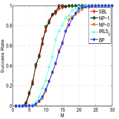
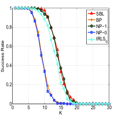
The success rate in the Fig. 3 is defined by the average probability of successful restoration, which is counted as the ratio between the number of successful trials and the total number of the independent experiments. It collects the result of 300 Monte Carlo trials and we assume successful trial if 𝐱^𝐱2/𝐱2<103subscriptnorm^𝐱𝐱2/subscriptnorm𝐱2superscript103{{{{\left\|{{\bf{\hat{x}}}-{\bf{x}}}\right\|}_{2}}}\mathord{\left/{\vphantom{{{{\left\|{{\bf{\hat{x}}}-{\bf{x}}}\right\|}_{2}}}{{{\left\|{\bf{x}}\right\|}_{2}}}}}\right.\kern-1.2pt}{{{\left\|{\bf{x}}\right\|}_{2}}}}<{10^{-3}}, where 𝐱^^𝐱{{\bf{\hat{x}}}} is the estimate of the original signal 𝐱𝐱\bf{x}. The mean squared error (MSE) in Fig. 4 which measures the average of the squares of the difference between the estimator and estimated signal is calculated as follow:

MSE(dB)=20log(𝐱^𝐱2/𝐱2)𝑀𝑆𝐸𝑑𝐵20subscriptnorm^𝐱𝐱2/subscriptnorm𝐱2MSE(dB)=20\log({{{{\left\|{{\bf{\hat{x}}}-{\bf{x}}}\right\|}_{2}}}\mathord{\left/{\vphantom{{{{\left\|{{\bf{\hat{x}}}-{\bf{x}}}\right\|}_{2}}}{{{\left\|{\bf{x}}\right\|}_{2}}}}}\right.\kern-1.2pt}{{{\left\|{\bf{x}}\right\|}_{2}}}})

Fig. 3 demonstrats the superior performance of the NP-1 algorithm in a few measurements. It shows the success rate of respective algorithms versus the number of measurement M and sparse level K of the signal. We can see that the reconstruction performance of the one layer normal product algorithm(NP-0) is almost the same as BP, which is the MAP estimation of unknowns in the one layer Laplace prior framework. The comparisons also show that the two layers normal product algorithm(NP-1) requires as few number of CS measurements as SBL while inheriting the similar reconstruction precision.

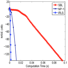
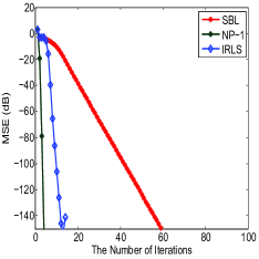
In Fig. 4, the comparison among the computational cost of the three algorithms on the reconstruction performance are performed on a personal PC with dual-core 3.1 GHz CPU and 4GB RAM. It is interesting to note that the MSE of NP-1 descends faster than SBL in Fig. 4(a) while it has the same sparsity-undersampling tradeoff performance as SBL. It should also be noticed that we haven’t use any basis pruning technology as in [16] to reduce the computational complexity. To understand the reason of low computational time from Fig. 4(b), we observe that the NP-1 requires only a few numbers of iterations to arrive at stop condition. In summary, these experimental results confirm that the NP-1 is a fast Sparse Bayesian algorithm.
Refer to caption
(a) K=3
Refer to caption
(b) M=30
Figure 3: Simulation results of Success Rate
Refer to caption
(a) K=3,M=30
Refer to caption
(b) K=3,M=30
Figure 4: Simulation results of Computational Cost

V Conculsion

In this letter, we formulated a Normal Product prior based Bayesian framework to solve the compressed sensing problem in noise free case. Using this framework, we derived two algorithms named NP-0 and NP-1 and compared them with different algorithms. We have shown that our algorithm NP-1 has the similar reconstruction performance with SBL while the interleaved updating procedure provides improved performance in computational times.

References

  • [1] D. L. Donoho, “Compressed sensing,” IEEE Trans. Inf. Theory, vol. 52, no. 4, pp. 1289–1306, 2006.
  • [2] E. J. Candès, J. Romberg, and T. Tao, “Robust uncertainty principles: Exact signal reconstruction from highly incomplete frequency information,” IEEE Tran. Inf. Theory, vol. 52, no. 2, pp. 489–509, 2006.
  • [3] J. A. Tropp and A. C. Gilbert, “Signal recovery from random measurements via orthogonal matching pursuit,” IEEE Trans. Inf. Theory, vol. 53, no. 12, pp. 4655–4666, 2007.
  • [4] S. S. Chen, D. L. Donoho, and M. A. Saunders, “Atomic decomposition by basis pursuit,” SIAM J. Sci. Comput., vol. 20, no. 1, pp. 33–61, 1998.
  • [5] R. Chartrand, “Exact reconstruction of sparse signals via nonconvex minimization,” IEEE Signal Process. Lett., vol. 14, no. 10, pp. 707–710, 2007.
  • [6] M. E. Tipping, “Sparse bayesian learning and the relevance vector machine,” J. Mach. Learn. Res., vol. 1, pp. 211–244, 2001.
  • [7] S. Ji, Y. Xue, and L. Carin, “Bayesian compressive sensing,” IEEE Trans. Signal Process., vol. 56, no. 6, pp. 2346–2356, 2008.
  • [8] D. P. Wipf and B. D. Rao, “Sparse bayesian learning for basis selection,” IEEE Trans. Signal Process., vol. 52, no. 8, pp. 2153–2164, 2004.
  • [9] S. D. Babacan, R. Molina, and A. K. Katsaggelos, “Bayesian compressive sensing using laplace priors,” IEEE Trans. Image Process., vol. 19, no. 1, pp. 53–63, 2010.
  • [10] E. W. Weisstein. Normal product distribution. MathWorld–A Wolfram Web Resource. [Online]. Available: http://mathworld.wolfram.com/NormalProductDistribution.html
  • [11] A. SEIJAS-MACÍAS and A. OLIVEIRA, “An approach to distribution of the product of two normal variables.” Discussiones Mathematicae: Probability & Statistics, vol. 32, 2012.
  • [12] D. Wipf, J. Palmer, and B. Rao, “Perspectives on sparse bayesian learning,” Computer Engineering, vol. 16, no. 1, p. 249, 2004.
  • [13] D. G. Tzikas, C. Likas, and N. P. Galatsanos, “The variational approximation for bayesian inference,” IEEE Signal Process. Mag., vol. 25, no. 6, pp. 131–146, 2008.
  • [14] I. F. Gorodnitsky and B. D. Rao, “Sparse signal reconstruction from limited data using focuss: A re-weighted minimum norm algorithm,” IEEE Trans. Signal Process., vol. 45, no. 3, pp. 600–616, 1997.
  • [15] R. Chartrand and W. Yin, “Iteratively reweighted algorithms for compressive sensing,” in Proc. ICASSP, 2008, pp. 3869–3872.
  • [16] M. E. Tipping, A. C. Faul et al., “Fast marginal likelihood maximisation for sparse bayesian models,” in Proc. 9th Int. Workshop on AIStats, vol. 1, no. 3, 2003.