Quantum fields as deep learning

Abstract

In this essay we conjecture that quantum fields such as the Higgs field is related to a restricted Boltzmann machine for deep neural networks. An accelerating Rindler observer in a flat spacetime sees the quantum fields having a thermal distribution from the quantum entanglement, and a renormalization group process for the thermal fields on a lattice is similar to a deep learning algorithm. This correspondence can be generalized for the KMS states of quantum fields in a curved spacetime like a black hole.

I Introduction

Recently, there is a growing interest in deep learning technology in high energy physics, in the hope that deep learning tools can provide significant boost in finding new particles at accelerators Baldi et al. (2014). Deep neural networks (DNN) and the restricted Boltzmann machine (RBM)  Hinton and Salakhutdinov (2006) show unprecedent power in pattern recognitions and unsupervised learning with complex big data. However, the reason why deep learning can outperform other machine learning techniques in extracting features is still unclear. One physical explanation is based on the analogy between the renormalization group (RG) and RBM Mehta and Schwab (2014). According to the explanation RBM can mimic the coarse-graining process of RG for a thermal system and this gives the efficient main feature extraction.

Linking information science to physics is a big trend in physics nowadays. For example, quantum entanglement is suggested to be a source of dark energy Lee et al. (2007), gravity Lee et al. (2013); Van Raamsdonk (2017) and the spacetime itself Van Raamsdonk (2010). Interestingly the holographic principle ’t Hooft (1993) as the AdS/CFT correspondence  Aharony et al. (2000) can be also related to entanglement Ryu and Takayanagi (2006) and RBM Gan and Shu (2017). Motivated by these works, in this paper we suggest that quantum field theory (QFT) can be interpreted to be a RBM and DNN. In Sec. II we review the relation between RG and RBM. In Sec. III an analogy between QFT and RBM is proposed. Section IV contains discussions.

II Renormalization group and Restricted Boltzmann machine

Let us briefly review the equivalence between RG and RBM Mehta and Schwab (2014) of deep learning using $N$ binary spins $\mathbf{v}=\{v_{i}\}$ ($i=1,2\cdots N$) in the Boltzmann distribution

$$P(\mathbf{v})=\frac{e^{-\mathbf{H}(\mathbf{v})}}{\mathcal{Z}},$$ (1)

with the Hamiltonian

$$\mathbf{H}(\mathbf{v})=\sum_{i}K_{i}v_{i}+\sum_{ij}K_{ij}v_{i}v_{j}+\sum_{ijk}K_{ijk}v_{i}v_{j}v_{k}+\cdots,$$ (2)

where $K_{ijk\cdots}$ are coupling constants. Then, the partition function $\mathcal{Z}$ is

$$\mathcal{Z}=\mathrm{T}r_{v_{i}}e^{-\mathbf{H}(\mathbf{v})},$$ (3)

which leads to the free energy $F=-ln\mathcal{Z}$. After one step of renormalization one can get the effective Hamiltonian for coarse-grained block spins $\mathbf{h}=\{h_{j}\}$

$$\mathbf{H}^{RG}(\mathbf{h})=\sum_{i}\bar{K}_{i}h_{i}+\sum_{ij}\bar{K}_{ij}h_{i}h_{j}+\sum_{ijk}\bar{K}_{ijk}h_{i}h_{j}h_{k}+\cdots,$$ (4)

where $\bar{K}_{ijk\cdots}$ are renormalized coupling constants. Repeating the above process yields renormalization of the theory.

In the variational RG scheme one step of RG process is implemented by introducing a function $\mathbf{T}_{\lambda}$ with some parameter $\lambda$ which satisfies

$$e^{-\mathbf{H}_{\lambda}^{RG}(\mathbf{h})}\equiv\mathrm{T}r_{v_{i}}e^{\mathbf{T}_{\lambda}(\mathbf{v},\mathbf{h})-\mathbf{H}(\mathbf{v})},$$ (5)

and then integrating out $\mathbf{v}$. Here, the free energy for the coarse grained system

$$F_{\lambda}\equiv-ln(Tr_{h_{j}}e^{-\mathbf{H}_{\lambda}^{RG}(\mathbf{h})})$$ (6)

remains equal to $F$ for an exact RG process. To do this $\mathbf{T}_{\lambda}$ should have an appropriate form.

On the other hand, Boltzmann machines are stochastic neural networks which can generate specific distribution of data. The restricted Boltzmann machine (RBM) is a version composed of visible units $\mathbf{v}$ and hidden units $\mathbf{h}$ having the following energy function describing the interaction between the visible and the hidden units,

$$\mathbf{E}(\mathbf{v},\mathbf{h})=\sum_{i}b_{i}v_{i}+\sum_{j}c_{j}h_{j}+\sum_{ij}w_{ij}v_{i}h_{j},$$ (7)

where the units in the same layer has no interaction between them, and $\lambda\equiv\{b_{i},c_{j},w_{ij}\}$ are variational parameters. The probability of a configuration of both units is given by

$$p_{\lambda}(\mathbf{v},\mathbf{h})=\frac{e^{-\mathbf{E}(\mathbf{v},\mathbf{h})}}{\mathcal{Z}},$$ (8)

and that of hidden units by

$$p_{\lambda}(\mathbf{h})=\sum_{\mathbf{v}}\frac{e^{-\mathbf{E}(\mathbf{v},\mathbf{h})}}{\mathcal{Z}}\equiv\frac{e^{-\mathbf{H}^{RBM}_{\lambda}(\mathbf{h})}}{\mathcal{Z}},$$ (9)

which leads to the definition of the Hamiltonian for the hidden units $\mathbf{H}^{RBM}$.

An exact mapping between the variational RG and RBM can be achieved by choosing the following function  Mehta and Schwab (2014)

$$\mathbf{T}_{\lambda}(\mathbf{v},\mathbf{h})=-\mathbf{E}(\mathbf{v},\mathbf{h})+\mathbf{H}(\mathbf{v}).$$ (10)

Then, inserting this into Eq. (5) one can find from Eq. (9)

$$\mathbf{H}^{RG}_{\lambda}(\mathbf{h})=\mathbf{H}^{RBM}_{\lambda}(\mathbf{h}),$$ (11)

and similarly $\mathbf{H}^{RG}_{\lambda}(\mathbf{v})=\mathbf{H}^{RBM}_{\lambda}(\mathbf{v})$. This implies that one step of the variational RG with the spins $\mathbf{v}$ and $\mathbf{h}$ can be mapped to two layers made of units $\mathbf{v}$ and $\mathbf{h}$ of the RBM.

III Quantum field as neural networks

How can we relate RBM with quantum fields? Quantum fields have complex wavefunctional, hence usually do not have the Boltzmann distribution. But, if there is a causal horizon the fields can be thermal. For example, it is possible for an accelerating observer to see the flat spacetime vacuum state as a Boltzmann distribution, which is the Unruh effect.

Consider an observer with acceleration $a$ in $x_{1}$ direction with coordinates $(t,x_{1},x_{2},x_{3})$ in a flat spacetime, who observes a scalar field with Hamiltonian

$$H(\phi)=\int d^{3}x\left[\frac{1}{2}\left(\frac{\partial\phi}{\partial t}\right)^{2}+\frac{1}{2}\left({\nabla\phi}\right)^{2}+V(\phi)\right]$$ (12)

with potential $V$. The field could be the standard model Higgs, inflaton or ultra-light scalar dark matter Lee (2017). The Rindler coordinates $(\eta,r,x_{2},x_{3})$ can be defined with

$$t=r~{}sinh(a\eta),~{}x_{1}=r~{}cosh(a\eta)$$ (13)

on the Rindler wedges.

In the Rindler coordinates the proper time interval is $ard\eta$ and hence the corresponding Hamiltonian becomes

$$H_{R}=\int drdx_{\bot}~{}ar\left[\frac{1}{2}\left(\frac{\partial\phi}{ar\partial\eta}\right)^{2}+\frac{1}{2}\left(\frac{\partial\phi}{\partial r}\right)^{2}+\frac{1}{2}\left({\nabla_{\bot}\phi}\right)^{2}+V(\phi)\right],$$ (14)

where $\bot$ denotes the spatial direction orthogonal to $(\eta,r)$. Then, the Rinder observer sees a horizon at $r=0$.

It is well-known that we can decompose the fields in the left and right Rindler wedges as $\phi_{L}$ and $\phi_{R}$, respectively, and the ground state of $H_{R}$ is then described by a wavefunctional

$$\Psi_{0}(\phi_{L},\phi_{R})=\frac{1}{\sqrt{\mathcal{Z}}}\langle\phi_{L}|e^{-\pi H_{R}}|\phi_{R}\rangle.$$ (15)

The two fields are entangled, and the reduced density matrix for $\phi_{R}$ is given by partial tracing $\phi_{L}$, i.e., $\rho_{R}=Tr_{\phi_{L}}\Psi_{0}\Psi_{0}^{\dagger}=\frac{1}{Z}exp(-2\pi H_{R})$. With the proper redshifted Unruh temperature $T=a/2\pi$ this density matrix becomes

$$\rho_{R}=\frac{1}{\mathcal{Z}}exp(-H_{R}/T),$$ (16)

which means $\phi_{R}$ has a Boltzmann distribution, and the Minkowski vacuum restricted to the one Rindler wedge is a KMS state  Ross (2005).

Now, we suggest that the quantum fields $\phi_{R}$ can be treated as a continuous version of $\mathbf{v}$, and $H_{R}$ can be $\mathbf{H}(\mathbf{v})$ in Eq. (2) for RBM. Recall that the RG process is a natural process in QFT. We propose that the coarse graining process for the quantum field corresponds to the information propagation in the deep neural networks. To be specific, let us consider a discretized spacetime with the minimum length scale $l$ of order of the Planck scale as in the lattice field theory. We also assume a quadratic potential with mass $m$. Then, in $d+1$ spacetime with a field $\phi_{R}$ at the site $x$, $\phi_{x}$,

$$H_{R}\simeq N_{1}l^{d+1}\sum_{r}ar\sum_{x}\left[\frac{(\phi_{x+\eta}-\phi_{x})^{2}}{2(arl)^{2}}+\sum_{\mu=1}^{d}\frac{(\phi_{x+\hat{\mu}}-\phi_{x})^{2}}{2l^{2}}+\frac{m^{2}\phi_{x}^{2}}{2}\right],$$ (17)

where $N_{1}$ is a normalization, $\hat{\mu}$ represents the unit vectors to the nearest points in the spatial direction $\mu$, and $\{x,r,\eta\}$ should be understood to be integer indexes ($r\geq 1$). With an appropriate $N_{1}$ we can rescale the field as $0\leq\phi_{x}\leq 1$. This can be justified because physical $\phi_{x}$ can not have an arbitrary large value, and hence there should be a maximum field value, say, of order of the Planck mass.

Now, with $H_{R}$ and $E(\mathbf{v},\mathbf{h})$ in Eq. (7) we can perform the one step of variational RG using Eq. (5). Here, the lattice field $\phi_{x}$ plays a role of the visible unit $v_{i}$ and renormalized field $\tilde{\phi}_{x}$ plays a role of the hidden unit $h_{j}$. At the next level $\tilde{\phi}_{x}$ acts as a new visible unit, and one can repeat the RG steps toward the IR limit. Therefore, the RG process for the scalar field corresponds to DNN and it is a kind of natural learning process. (See Fig. 1)

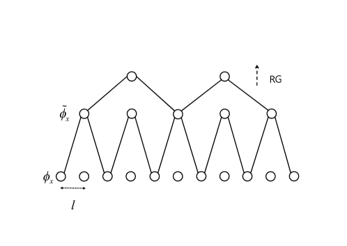
Figure 1: Quantum fields $\phi_{x}$ on a lattice with a UV-cutoff $l$ act as visible units. The solid lines represent $w_{ij}$. After one step of the variational RG with the decimation, the renormalized field $\tilde{\phi}_{x}$ plays a role of the hidden units. At the next level $\tilde{\phi}_{x}$ acts as a new visible units. The whole RG process then corresponds to DNN.

At each RG step, there is a coarsegraining of the field leading to effective field theory of the system. Like the output units in RBM, this effective field contain the concise information of the lower units, that is, UV-physics. This might explain why effective field theory is so successful to describe a low energy physics despite of partial information loss about the UV-phyics. Repeating the real space RG steps leads to the RG process toward an IR region, which corresponds to DNN. One can check the validity of this concept by reverting the process and approximately reproducing the input information (field values of the lowest units in the Fig. 1) from the output units (the most upper units) and the trained parameters $\{b_{i},c_{j},w_{ij}\}$. This corresponds to the inversion of the ordinary RG process in the field theory from IR to UV.

Further simplification can be done for a numerical study by considering an Rindler observer with a hugh acceleration $a\gg 1$. Then, we can ignore the time derivative term and get

$$H_{R}\simeq N_{1}\sum_{r}\frac{ar}{2}\sum_{x}\left[\sum_{\mu=1}^{d}{(\phi_{x+\hat{\mu}}-\phi_{x})^{2}}+{m^{2}\phi_{x}^{2}}\right],$$ (18)

where we set $l=1$. From the above equation we expect the thermal fluctuation of the field mainly exists near the horizon, i.e., $r\simeq 1$.

We have considered the vacuum state so far. For a slightly excited state $\Psi_{0}+\delta\Psi$, the initial density matrix and the probability distribution should be slightly changed. This effect can be reflected by including an interaction term $H_{int}$ into the Hamiltonian $H_{R}$ . Otherwise, if we keep $H_{R}$ fixed, $E(\mathbf{v},\mathbf{h})$ and the couplings $\{b_{i},c_{j},w_{ij}\}$ should be changed instead to represents the excited state. This might be another kind of natural learning process. Thus, we guess there is a mapping between quantum states not far from the vacuum state and information (i.e., parameters) in the corresponding RBM model.

It is straightforward to extend the previous arguments to a black hole case. For the Schwarzchild black holes with mass $M$ the metric is given by

$$ds^{2}=-Fdt^{2}+F^{-1}dr^{2}+r^{2}d\Omega^{2},$$ (19)

where $F=1-2GM/r$. Near the event horizon this reduces to the Rindler metric

$$ds^{2}\simeq-R^{2}d\eta^{2}+dR^{2}+r^{2}d\Omega^{2},$$ (20)

with $R=\sqrt{r(r-2MG)}$ and $\eta=t/4GM$ as is well-known. Therefore, we expect quantum fields near the black hole horizon is also a KMS state and can be viewed as a DNN for a observer seeing the Hawking radiation.

IV Discussions

Yet another possible approach is to use the well-known correspondence of the Euclidean quantum field theory in $d+1$ dimensional flat spacetime and the statistical mechanics in $d+1$ dimensional flat space using an imaginary time. In this case we do not need an accelerating observer. The Euclidean functional integral

$$\mathcal{Z}=\int d\phi e^{-\int d^{d+1}x~{}H(\phi)/\hbar}$$ (21)

has the form of the partition function for the classical thermal system with $T=\hbar$ and one can now easily see the analogy to DNN.

It would be easy to extend our arguments to the KMS states of other spin fields such as fermions, gauge vectors, and gravitons with causal horizons. The unexpected relation between the quantum field and DNN might explain why DNN is so successful in particle identification at accelerator experiments  Baldi et al. (2014). Conversely, QFT can give some insights to understand why RBM is so powerful.

Our conjecture also implies a surprising possibility that the quantum fields, and hence matter in the universe, can memorize information and even can perform self-learning to some extend like DNN in a way consistent with the Strong Church-Turing thesis.