Two efficient computational algorithms to solve the singularly perturbed Lane-Emden problem

Abstract

In this paper, we decide to compare two new approaches based on Rational and Exponential Bessel functions (RBs and EBs) to solve several well-known class of Lane-Emden type models. The problems, which define in some models of non-Newtonian fluid mechanics and mathematical physics, are nonlinear ordinary differential equations of second-order over the semi-infinite interval and have singularity at $x=0$. We have converted the non-linear Lane-Emden equation to a sequence of linear equations by utilizing the quasilinearization method (QLM) and then, these linear equations have been solved by RBs and EBs collocation-spectral methods. Afterward, the obtained results are compared with the solution of other methods for demonstrating the efficiency and applicability of the proposed methods.

1 Introduction

The investigation of a singular initial/boundary value non-linear differential equations of second-order have been attracted by some astrophysicist, mathematicians and physicists. Lane-Emden type equations describe the temperature variation of a spherical gas cloud under the mutual attraction of its molecules and subject to the laws of classical thermodynamics. Let $P(r)$ denote the total pressure at a distance $r$ from the center of spherical gas cloud. The total pressure is due to the usual gas pressure and a contribution from radiation:

$$P=(\frac{1}{3}\xi T^{4}+\frac{RT}{v}),$$

where $\xi,T,R$ and υ are respectively the radiation constant, the absolute temperature, the gas constant, and the specific volume, respectivelyrefff03 ; refff04 . Let $M(r)$ be the mass within a sphere of radius $r$ and $G$ the constant of gravitation. The equilibrium equation for the configuration are

$$\frac{dP}{dr}=-\rho\frac{GM(r)}{r^{2}},$$ (1)

$$\frac{dM(r)}{dr}=4\pi\rho r^{2},$$

where $\rho$, is the density, at a distance $r$, from the center of a spherical star. Eliminating $M$ yields of these equations results in the following equation, which as should be noted, is an equivalent form of the Poisson equation refff04 ; refff05 :

$$\frac{1}{r^{2}}\frac{d}{dr}(\frac{r^{2}}{\rho}\frac{dP}{dr})=-4\pi G\rho.$$

We already know that in the case of a degenerate electron gas, the pressure and density are$\rho=P^{\frac{3}{5}}$, assuming that such a relation exists in other states of the star, we are led to consider a relation of the form $P=K\rho^{1+\frac{1}{m}}$, where $K$ and $m$ are constants.

We can insert this relation into Eq.(1) for the hydrostatic equilibrium condition and, from this, we can rewrite the equation as follows:

$$\Bigg{[}\frac{K(m+1)}{4\pi G}\lambda^{\frac{1}{m}-1}\Bigg{]}\frac{1}{r^{2}}\frac{d}{dr}(r^{2}\frac{dy}{dr})=-y^{m},$$

where $\lambda$ represents the central density of the star and y denotes the dimensionless quantity, which are both related to $\rho$ through the following relation refff01 ; refff05 :

$$\rho=\lambda y^{m}(x),$$

and let

$$r=ax,$$

$$a=\Bigg{[}\frac{K(m+1)}{4\pi G}\lambda^{\frac{1}{m}-1}\Bigg{]}^{\frac{1}{2}}.$$

Inserting these relations into our previous relation we obtain the Lane-Emden equation refff04 ; refff05 :

$$\frac{1}{x^{2}}\frac{d}{dx}(x^{2}\frac{dy}{dx})=-y^{m},$$

now, we will have the standard Lane-Emden equation with $f(x,y)=y^{m}$

$$y^{\prime\prime}(x)+\frac{2}{x}y^{\prime}(x)+y^{m}(x)=0,~{}~{}x>0,$$ (2)

the initial conditions are as follows

$$y(0)=1~{},~{}y^{\prime}(0)=0.$$ (3)

The values of $m$, which are physically interesting, lie in the interval [0, 5]. The main difficulty in analyzing this type of equation is the singularity behaviour occurring at $x=0$.

As it has been mentioned in the literature review, the solutions of the Lane-Emden equation could be exact only for $m=0,1$ and $5$. For the other values of $m$, the Lane- Emden equation is to be integrated numerically refff05 . Thus, we decided to present a new and efficient technique to solve it numerically for $m=0.5,1.5,2,2.5,3,3.5$ and $4$.

1.1 Previous works

Recently, many analytical, semi- analyticaland and numerical techniques have been applied to solve Lane-Emden equations. The main difficulty arises in the singularity of the equations at $x=0$. We have introduced several techniques as follow:

Bender et al. refff06 proposed a new perturbation technique based on an artificial parameter $\delta$, the method is often called $\delta$-method. Wazwaz refff08 employed the Adomian decomposition technique with an alternate framework designed, J.H. He refff11 employed Ritz’s method to obtain an analytical solution, Parand et. al. refff15 ; refff16 ; refff17 ; refff18 ; refff19 applied pseudo-spectral method based on rational Legendre functions, Sinc collocation method, the Lagrangian method based on modified generalized Laguerre function, Hermite function collocation method and meshless collocation method based on Radial basis function (RBs) as numerical solution, Ramos refff20 ; refff21 ; refff22 ; refff23 presented linearzation methods to utilize an analytical solutions and globally smooth solutions, developed piecewise-adaptive decomposition methods, obtained series solutions of the Lane-Emden type equation, Yousefi refff24 applied Legendre Wavelet approximations and used integral operator and converted Lane-Emden equations to integral equations, Chowdhury and Hashim refff25 used analytical solutions of the generalized Emden- Fowler type equations by homotopy perturbation method (HPM), Aslanov refff27 introduced a further development in the Adomian decomposition technique, Dehghan and Shakeri refff28 investigated Lane-Emden equations by applying the variational iteration method, Marzban et al. refff30 used a method based upon hybrid of block-pulse functions and Lagrange interpolating polynomials together with the operational integration matrix to approximate solution of the problem, Adibi and Rismani in refff31 proposed the approximate solutions of singular the Lane-Emden via modified Legenre-spectral method, Karimi vanani and Aminataei refff32 provided a numerical method which produces an approximate polynomial solution, thesy used an integral operator and convert Lane-Emden equations into integral equations then, convert the acquired integral equations into a power series and finally, transforming the power series into padé series form, Kaur et al. refff33 obtained the Haar wavelet approximate solution.

So, the other researchers trying to solving the Lane-Emden type equations with several methods, For example, A Yildirım and Öziş refff34 ; refff35 by using HPM and VIM methods, Benko et al. refff36 by using Nyström method, Iqbal and javad refff37 by using Optimal HAM, Boubaker and Van Gorder refff38 by using boubaker polynomials expansion scheme, Daşcıoǧlu and Yaslan refff39 by using Chebyshev collocation method, Yüzbaşı refff40 ; refff41 by using Bessel matrix and improved Bessel collocation method, Boyd refff42 by using Chebyshev spectral method, Bharwy and Alofi refff43 by using Jacobi-Gauss collocation method, Pandey et al. refff44 ; refff45 by using Legendre and Brenstein operation matrix, Rismani and monfared refff46 by using Modified Legendre spectral method, Nazari-Golshan et al. refff47 by using Homotopy perturbation with Fourier transform, Doha et al. refff48 by using second kind Chebyshev operation matrix algorithm, Carunto and bota refff49 by using Squared reminder minimization method, Mall and Chakaraverty refff50 by using Chebyshev Neural Network based model, Gürbüz and sezer refff51 by using Laguerre polynomial and Kazemi-Nasab et al. refff52 by using Chebyshev wavelet finite difference method. In this paper, we attempt to introduce a new method, based on RBF-DQ for solving non-linear ODEs.

The rest of this paper is arranged as follows:

Section 2 introduces new rational and exponential Bessel functions (RBs and EBs) and their properties. Section 3 describes a brief formulation of quasilinearization method (QLM) introduced by QLM03 . In section 4 at first, by utilizing QLM over Lane-Emden equation a sequence of linear differential equations is obtained, then at each iteration solve the linear differential equation by RBs and EBs collocation methods that we name RBs-QLM and EBs-QLM methods. Comparison between these two methods with some well-known results in section 5, show that using rational functions is highly accurate, and we also describe our results via tables and figures. Finally, we give a brief conclusion in section 6.

2 Properties of Rational and Exponential Bessel Functions

The Bessel functions arise in many problems in physics possessing cylindrical symmetry, such as the vibrations of circular drumheads and the radial modes in optical fibers. Bessel functions are usually defined as a particular solution of a linear differential equation of the second order which known as Bessel’s equation. Bessel functions first defined by the Daniel Bernoulli on heavy chains (1738) and then generalized by Friedrich Bessel. More general Bessel functions were studied by Leonhard Euler in (1781) and in his study of the vibrating membrane in (1764) reffff01 ; reffff02 .

Bessel differential equation of order $n\in\mathbb{R}$ is:

$$x^{2}\frac{d^{2}y(x)}{dx^{2}}+x\frac{dy(x)}{dx}+(x^{2}-n^{2})y(x)=0,~{}~{}x\in(-\infty,\infty).$$ (4)

One of the solutions of equation (4) by applying the method of Frobenius as follows reffff03 :

$$J_{n}(x)=\sum_{r=0}^{\infty}\frac{(-1)^{r}}{r!(n+r)!}(\frac{x}{2})^{2r+n},$$ (5)

where series (5) is convergent for all $x\in(-\infty,\infty)$.

polynomials has been introduced as follows reffff11 ; reffff12 :

$$B_{n}(x)=\sum_{r=0}^{[\frac{N-n}{2}]}\frac{(-1)^{r}}{r!(n+r)!}(\frac{x}{2})^{2r+n},~{}~{}x\in[0,1].$$ (6)

where $n\in\mathbb{N}$, and $N$ is the number of basis of Bessel polynomials.

2.1 Rational Bessel Functions

The new basis functions, ”Rational Bessel functions (RBs)” denote by $RB_{n}(x,L)$ which are generated from well known Bessel polynomials by using the algebraic mapping $\phi(x)=\frac{x}{x+L}$, as follow:

$$RB_{n}(x,L)=B_{n}(\phi(x))~{},~{}~{}n=0,1,\cdots,N$$

or

$$RB_{n}(x,L)=\sum_{r=0}^{[\frac{N-n}{2}]}\frac{(-1)^{r}}{r!(n+r)!}(\frac{x}{2(x+L)})^{2r+n},~{}~{}n=0,1,\cdots,N$$ (7)

where $x\in[0,\infty)$, $B_{n}(x)$ is Bessel polynomials of order $n$, and the constant parameter $L>0$ is a scaling/stretching factor which can be used to fine tune the spacing of collocation points. For a problem whose solution decays at infinity, there is an effective interval outside of which the solution is negligible, and collocation points which fall outside of this interval are essentially wasted. On the other hand, if the solution is still far from negligible at the collocation points with largest magnitude, one cannot expect a very good approximation. Hence, the performance of spectral methods in unbounded domains can be significantly enhanced by choosing a proper scaling parameter such that the extreme collocation points are at or close to the endpoints of the effective interval reffff17 . Boyd refdd26 offered guidelines for optimizing the map parameter $L$ for rational Chebyshev functions, which is also useful for RBs.

Let us define $\Gamma=\{x|~{}0\leq x<\infty\}$ and
$L^{2}_{w_{r}}(\Gamma)=\{~{}v:\Gamma\rightarrow\mathbb{R}|v$ is measurable and $\parallel v\parallel_{w_{r}}<\infty\}$, where

$$\parallel v\parallel_{w_{r}}=\left(\int^{\infty}_{0}|v(x)|^{2}w_{r}(x,L)dx\right)^{1/2},$$

with $w_{r}(x,L)=\frac{L}{(x+L)^{2}}$, is the norm induced by inner product of the space $L^{2}_{w_{r}}(\Gamma)$ as follows:

$$\langle v,u\rangle_{w_{r}}=\int^{\infty}_{0}{v(x)u(x)w_{r}(x,L)}dx.$$

Now, suppose that

$$\mathfrak{S}=~{}span\{RB_{0}(x),RB_{1}(x),\dots,RB_{N}(x)\},$$

where $\mathfrak{S}$ is a finite-dimensional subspace of $L^{2}_{w}(\Gamma)$, $dim(\mathfrak{S})=N+1$, so $\mathfrak{S}$ is a closed subspace of $L^{2}(\Gamma)$. Therefore, $\mathfrak{S}$ is a complete subspace of $L^{2}(\Gamma)$. Assume that $f(x)$ be an arbitrary element in $L^{2}(\Gamma)$. Thus $f(x)$ has a unique best approximation in $\mathfrak{S}$ subspace, say $\hat{b}(x)\in\mathfrak{S}$, that is

$$\exists~{}\hat{b}(x)\in\mathfrak{S},~{}~{}~{}\forall~{}b(x)\in\mathfrak{S}(x),~{}~{}\parallel f(x)-\hat{b}(x)\parallel_{w_{r}}\leq\parallel f(x)-b(x)\parallel_{w_{r}}.$$

Notice that we can write $b(x)$ vector as a combination of the basis vectors of $\mathfrak{S}$ subspace.

We know function of $f(x)$ can be expanded by $N+1$ terms of RB as:

$$f(x)=f_{N}(x)+R(x),$$

that is

$$f_{N}(x)=\sum^{N}_{n=0}{a_{n}RB_{n}(x)}=A^{T}RB(x),$$ (8)

where $RB(x)$ is vector $[RB_{0}(x),RB_{1}(x),\cdots,RB_{N}(x)]^{T}$ and $R\in\mathfrak{S}^{\perp}$ that ${\mathfrak{S}}^{\perp}$ is the orthogonal complement. So $f(x)-f_{N}(x)\in\mathfrak{S}^{\perp}$ and $b(x)\in\mathfrak{S}$ are orthogonal which we denote it by:

$$f(x)-f_{N}(x)\perp b,$$

thus $f(x)-f_{N}(x)$ vector is orthogonal over all of basis vectors of $\mathfrak{S}$ subspace as:

$$\langle f(x)-f_{N}(x),RB_{i}(x)\rangle_{w_{r}}=\langle f(x)-A^{T}RB(x),RB_{i}(x)\rangle_{w_{r}}=0,~{}i=0,1,\cdots,N,$$

hence

$$\langle f(x)-A^{T}RB(x),RB^{T}(x)\rangle_{w_{r}}=0,$$

therefore A can be obtained by

$$\langle f(x),RB^{T}(x)\rangle_{w_{r}}=\langle A^{T}RB(x),RB^{T}(x)\rangle_{w_{r}},$$

$$A^{T}=\langle f(x),RB^{T}(x)\rangle_{w_{r}}~{}\langle RB(x),RB^{T}(x)\rangle_{w_{r}}^{-1},~{}n=0,1,\cdots,N.$$

2.2 Exponentioal Bessel Functions

Exclusive of rational functions we can use exponential transformation to have new functions which are also defined on the semi-infinite interval. The exponential Bessel functions ($EBs$) can be defined by

$$EB_{n}(x)=B_{n}(1-e^{-x/L})~{},~{}~{}n=0,1,\cdots,N.$$

or

$$EB_{n}(x,L)=\sum_{r=0}^{[\frac{N-n}{2}]}\frac{(-1)^{r}}{r!(n+r)!}(1-e^{-x/L})^{2r+n},~{}~{}n=0,1,\cdots,N.$$ (9)

where parameter L is a constant parameter and, like rational functions, it sets the length scale of the mapping.

All of the above relations can also be used to EBs with respect to the weight function $w_{e}(x,L)=\frac{e^{-x/L}}{L}$ in the interval $[0,\infty)$.

3 The quasilinearization method (QLM)

The QLM is a generalization of the Newton-Raphson method QLM02 to solve the nonlinear differential equation as a limit of approximating the nonlinear terms by an iterative sequence of linear expressions. The QLM techniques are based on the linearization of the higher order ordinary/partial differential equation and require the solution of a linear ordinary differential equation at each iteration. Mandelzweig and Tabakin QLM05 have determined general conditions for the quadratic, monotonic and uniform convergence of the QLM method to solve both initial and boundary value problems in nonlinear ordinary $n$th order differential equations in $N$-dimensional space.

Let us assume that a second-order nonlinear ordinary differential equation in one variable on the interval $[0,\infty)$ as follows:

$$\frac{d^{2}u}{dx^{2}}=F(u^{\prime}(x),u(x),x),$$ (10)

with the boundary conditions: $u(0)=A,~{}u(\infty)=B$, where $A$ and $B$ are real constants and $F$ is nonlinear function.

By utilizing the QLM to solve Eq. (10) determines the $(I+1)$th iterative approximation $u_{I+1}(t)$ as a solution of the linear differential equation:

$$\frac{d^{2}u_{I+1}}{dx^{2}}=F(u^{\prime}_{r},u_{r},x)+(u_{I+1}-u_{r})F_{u}(u^{\prime}_{r},u_{r},x)+(u^{\prime}_{I+1}-u^{\prime}_{r})F_{u^{\prime}}(u^{\prime}_{r},u_{r},x),$$ (11)

with the boundary conditions:

$$u_{I+1}(0)=A,~{}~{}~{}~{}~{}u_{I+1}(\infty)=B,$$ (12)

where $~{}r=0,1,2,\cdots$ and the functions $F_{u}=\partial F/\partial u$ and $F_{u^{\prime}}=\partial F/\partial u^{\prime}$ are functional derivatives of functional $F(u^{\prime}_{r},u_{r},x)$.

4 Application of the Methods

In this paper, two methods based on RBs collocation method and EBs collocation method for solving Eq. (2), with initial conditions of Eq. (3), have been considered.

First, by utilizing QLM technique on Eq. (2), we have

$$xy^{\prime\prime}_{I+1}(x)+2y^{\prime}_{I+1}(x)-(m-1)xy^{m}_{I}(x)+mxy_{I+1}(x)y^{m-1}_{I}(x)=0$$ (13)

with the initial conditions:

$$y_{I+1}(0)=1,~{}~{}~{}~{}~{}~{}y^{\prime}_{I+1}(0)=0,$$ (14)

where $I=0,1,2,\cdots.$

For rapid convergence is actually enough that the initial guess is sufficiently good to ensure the smallness of just one of the quantity $q_{r}=k||y_{I+1}-y_{I}||$, where $k$ is a constant independent of $I$. Usually, it is advantageous that $y_{0}(t)$ would satisfy at least one of the initial conditions Eq. (3) QLM10 , thus set $y_{0}(x)=1$ for the initial guess of Lane-Emden equation.

Then, we can approximate $y_{I+1}(x)$ by $N+1$ basis of RBs and EBs as follows:

1. approximating $y_{I+1}(x)$ by $N+1$ basis of RBs:

   1. $$y_{I+1}(x)\thickapprox u_{N,I+1}(x)=1+x^{2}\sum^{N}_{n=0}{\hat{b_{n}}RB_{n}(x,L)}.$$ (15)

      where $r=0,1,2,\cdots.$ and two terms $1$ and $x^{2}$ are to satisfy initial conditions Eq. (14).

      To apply the collocation method, we have constructed the residual function for $(I+1)$th iteration in QLM by substituting $y_{I+1}(x)$ by $u_{N,I+1}(x)$ into Eq. (13) as following:

      $$RESr_{I+1}(x)=xu^{\prime\prime}_{N+1,I+1}(x)+2u^{\prime}_{N+1,I+1}(x)$$

      $$-(m-1)xu^{m}_{N+1,I}(x)+mxu_{N+1,I+1}(x)u^{m-1}_{N+1,I}(x)=0$$ (16)

2. approximating $y_{I+1}(x)$ by $N+1$ basis of EBs:

3. $$y_{I+1}(x)\thickapprox w_{N,I+1}(x)=\frac{1}{x^{2}+1}+\frac{x^{2}}{x+1}\sum^{N}_{n=0}{\hat{c_{n}}EB_{n}(x,L)}.$$ (17)

   where $r=0,1,2,\cdots.$
   In this paper, we have been considered two terms $\frac{1}{x^{2}+1}$ and $\frac{x^{2}}{x+1}$ to satisfy initital conditions Eq. (14).
   Also, like above, to apply the collocation method, we have constructed the residual function for $(I+1)$th iteration in QLM by substituting $y_{I+1}(x)$ by $w_{N,I+1}(x)$ into Eq. (13) as following:

   $$RESe_{I+1}(x)=xw^{\prime\prime}_{N+1,I+1}(x)+2w^{\prime}_{N+1,I+1}(x)$$

   $$-(m-1)xw^{m}_{N+1,I}(x)+mxw_{N+1,I+1}(x)w^{m-1}_{N+1,I}(x)=0$$ (18)

In all of the spectral methods, the purpose is to find $\hat{b_{n}}$ and $\hat{c_{n}}$ coefficients.

A method for forcing the residual functions Eq. (1) and Eq. (4) to zero can be defined as collocation algorithm. There is no limitation to choose the point in collocation method. The $N+1$ collocation points have been substituted in $RESr_{I+1}(x)$ and $RESe_{I+1}(x)$ equations, therefore:

$$RESr_{I+1}(x_{i})=0,~{}~{}i=0,1,,\cdots,N+1.$$ (19)

$$RESe_{I+1}(x_{i})=0,~{}~{}i=0,1,,\cdots,N+1.$$ (20)

which $x_{i}$ are roots of the shifted Chebyshev functions on finite intervalrefdd27 . Finally, a linear system of equations has been obtained, all of these equations can be solved by Newton method for the unknown coefficients.

5 Results and discussion

The Lane-Emden type describe the variation of density as a function of the radial distance for a polytrope. They was first studied by the astrophysicists Jonathan Homer Lane and Robert Emden, which considered the thermal behavior of a spherical cloud of gas acting under the mutual attraction of its molecules and subject to the classical laws of thermodynamicsrefff01 ; refff02 . In the Lane-Emden type equations, the first zero of $y(x)$ is an important point of the function, so we have computed $y(x)$ to this zero. In this paper, the equation is solved for $m=1.5,2,2.5,3$ and $4$, which does not have exact solutions.
The comparison of the initial slope $y^{\prime}(0)$ calculated by RBs-QLM with values obtained by Horedtrefff05 is given in table 1.
Table 2 and 3 have presented some numerical examples to illustrate the accuracy and convergence of our suggested methods by increasing the number of points and iterations.
Tables 4, 5, 6, 7 and 8 show the obtained values of $y(x)$ and $y^{\prime}(x)$ by the approch which based on RBs collocation method, for $m=1.5,2,2.5,3$ and $4$ with values of $N=75$ and iteration 15.
The resulting graphs of the standard Lane-Emden equation obtained by present methods for $m=1.5,2,2.5,3$ and $4$ are shown in figure 1.
Finally, figures 2, 3, 4, 5 and 6 show the residual errors for approximation solutions by basis of rational and exponential function with $N=50,75$ and 100. note that the residual error decreases with the increase of the collocation points.

6 Conclusion

The fundamental goal of this paper were to introduce novel hybrid basis of Rational Bessel and Exponential functions (RB, EBs) with quasilinearization meyhod (QLM) to construct an approximation for solving nonlinear Lane-Emden type equations. These problems describe a variety of phenomena in theoretical physics and astrophysics, including aspects of stellar structure, the thermal history of a spherical cloud of gas, isothermal gas spheres, and thermionic currents refff04 . To achieve these goal at first, a sequence of linear differential equations is obtained by utilizing QLM over Lane-Emden equation. Second, in each iteration of QLM, the linear differential equation is solved by new RBs and EBs collocation method. This paper has been shown that the present works have provided two acceptable approaches for solving Lane-Emden type equations coused by the following reasons:

• Cause of simplicity to solve problems and convergence of approximation functions, we convert the nonlinear problems to a sequence linear equations using QLM

• Numerical results indicate effectiveness, applicability and accuracy of the present approaches.

• Present paper described shortly bibliography of different methods utilizined previous works for solving Lane-Emden-type equations.

• The approaches applied to solve the problems without reformulating the equation to bounded domains.

• The approaches have been displyed converges when increasing the number of collocation points by tabular reports.

• At the first time, Rational Bessel and Exponential functions have been to obtain numerical outcomes of the nonlinear exponent $m$ of the standard Lane-Emden equations.

• Moreover, a very good approximation solution of $y(x)$ for Lane-Emden type equations with various value of parameter $m$ after only fifteen iterations are obtained. So, these methods are a good experience and method for the other sciences.

.

(a) rational

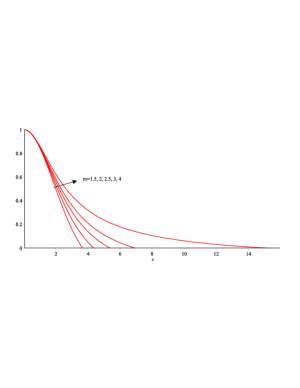
(b) exponential

Figure 1: The obtained graphs of solutions of Lane-Emden standard equations by basis of RBs and EBs with $m=1.5,2,2.5,3,4$

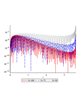
(a) rational

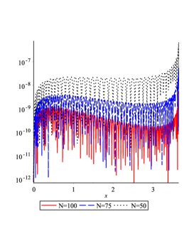
(b) exponential

Figure 2: Logarithmic graph of residual error by present works with $N=50,75,100$ and iteration 15 when m=1.5.

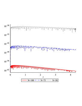
(a) rational

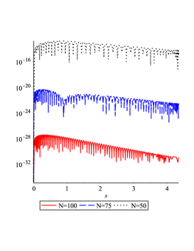
(b) exponential

Figure 3: Logarithmic graph of residual error by present works with $N=50,75,100$ and iteration 15 when m=2.

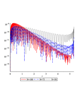
(a) rational

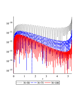
(b) exponential

Figure 4: Logarithmic graph of residual error by present works with $N=50,75,100$ and iteration 15 when m=2.5.

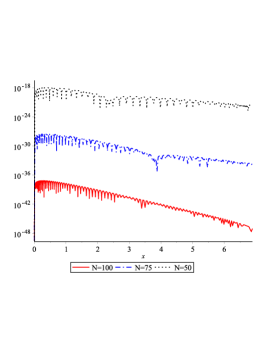
(a) rational

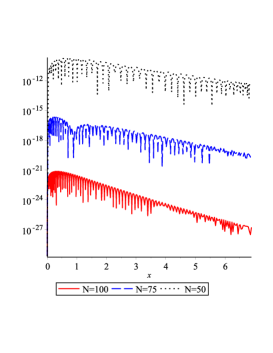
(b) exponential

Figure 5: Logarithmic graph of residual error by present works with $N=50,75,100$ and iteration 15 when m=3.

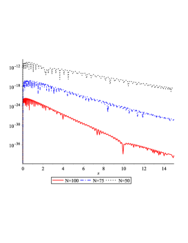
(a) rational

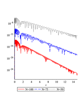
(b) exponential

Figure 6: Logarithmic graph of residual error by present works with $N=50,75,100$ and iteration 15 when m=4.

Table 1: Comparison of the first zeros of standard Lane-Emden equations, for numerical values given by Horedtrefff05 nad the present methods with N=75 and iteration 15

$m$	RBs	EBs	Horedt refff05
1.5	3.65375373622763424836747856706295570	3.653753736227530116708951	3.65375374
2.0	4.35287459594612467697357006152614262	4.352874595946124676973570	4.35287460
2.5	5.35527545901076012377857991160851840	5.355275459010769844745925	5.35527546
3.0	6.89684861937696037545452818712314053	6.896848619376960375436984	6.89684862
4.0	14.9715463488380950976509645543077611	14.97154634883796085494984	14.9715463

Table 2: Numerical results of first zeros by basis of RBs with various values of $m$, $N$ and iterations, accurate digits are bold

$m$	$N$	iteration	RBs
1.5	50	05	3.65375373625072342590
		10	3.65375373625071853754
		15	3.65375373625071853754
		20	3.65375373625071853754
	75	05	3.65375373622763914172
		10	3.65375373622763424836
		15	3.65375373622763424836
		20	3.65375373622763424836
	100	05	3.65375373622225950682
		10	3.65375373622225461061
		15	3.65375373622225461061
		20	3.65375373622225461061
2	50	05	4.3541023191782544510394699271974639349588062470049419121696397470
		10	4.35287459594612467697357006152614339487342457587311708331752
		15	4.35287459594612467697357006152614339487342457587311708331752
		20	4.35287459594612467697357006152614339487342457587311708331752
	75	05	4.352874597893199784546816142774753394907169932534281348066892095
		10	4.352874595946124676973570061526142628112365363213147181521
		15	4.352874595946124676973570061526142628112365363213147181521
		20	4.352874595946124676973570061526142628112365363213147181521
	100	05	4.352874597893199784546816142774753394907169932542963806389373524
		10	4.352874595946124676973570061526142628112365363213008835302
		15	4.352874595946124676973570061526142628112365363213008835302
		20	4.352874595946124676973570061526142628112365363213008835302
2.5	50	05	5.3552964545076443677
		10	5.355275459010744925
		15	5.355275459010744925
		20	5.355275459010744925
	75	05	5.35529645450764436772
		10	5.3552754590107601237
		15	5.3552754590107601237
		20	5.3552754590107601237
	100	05	5.35529645450764436772
		10	5.3552754590107873176
		15	5.3552754590107873176
		20	5.3552754590107873176
3	50	05	7.1216938046517305045330727094680858444666907392
		10	6.8968486193769603754542796110144170369244612
		15	6.8968486193769603754542796110144170369244612
		20	6.8968486193769603754542796110144170369244612
	75	05	7.1216938046404145204995503800811081360235860196
		10	6.89684861937696037545452818712314053555203
		15	6.89684861937696037545452818712314053555203
		20	6.89684861937696037545452818712314053555203
	100	05	7.1216938046404152911963760032858519494248670403
		10	6.89684861937696037545452818712312127697218
		15	6.89684861937696037545452818712312127697218
		20	6.89684861937696037545452818712312127697218
4	50	05	16.711045707072842315340457798698905988740559701
		10	14.97154867059731700938111496437106672775015032
		15	14.9715463488382089901971898981867391578167481
		20	14.9715463488382089901971898981867391578167481
	75	05	16.402670239960775259418702056564527058250944781
		10	14.97154289318059650158197244640609252173187180
		15	14.971546348838095097650964554307761107155441
		20	14.971546348838095097650964554307761107155441
	100	05	16.172787459355139190211994543646969560813181439
		10	14.97154439717955256111887952830248179390503419
		15	14.971546348838095097611066133148254587457821
		20	14.971546348838095097611066133148254587457821

Table 3: Numerical results of first zeros by basis of EBs with various values of $m$, $N$ and iterations, accurate digits are bold

$m$	$N$	iteration	EBs
1.5	50	05	3.65375373625083916424
		10	3.65375373625083427589
		15	3.65375373625083427589
		20	3.65375373625083427589
	75	05	3.65375373622753501010
		10	3.65375373622753011670
		15	3.65375373622753011670
		20	3.65375373622753011670
	100	05	3.65375373622227432714
		10	3.65375373622226943093
		15	3.65375373622226943093
		20	3.65375373622226943093
2	50	05	4.352874597893199785338903310594652764
		10	4.35287459594612467776565735834309221
		15	4.35287459594612467776565735834309221
		20	4.35287459594612467776565735834309221
	75	05	4.35287459594612467697472244822039342
		10	4.3528745959461246769735701033024306
		15	4.3528745959461246769735701033024306
		20	4.3528745959461246769735701033024306
	100	05	4.3528745978931997845468161427747526020
		10	4.3528745959461246769735700615261418
		15	4.3528745959461246769735700615261418
		20	4.3528745959461246769735700615261418
2.5	50	05	5.35529645450764438595
		10	5.3552754590107203902
		15	5.3552754590107203902
		20	5.3552754590107203902
	75	05	5.35529645450764436772
		10	5.3552754590107698447
		15	5.3552754590107698447
		20	5.3552754590107698447
	100	05	5.35529645450764436772
		10	5.3552754590107770840
		15	5.3552754590107770840
		20	5.3552754590107770840
3	50	05	7.12169371888993111013538427437823
		10	6.896848619376969505160794512467
		15	6.896848619376969505160794512467
		20	6.896848619376969505160794512467
	75	05	7.12169380466912339539903047482119
		10	6.89684861937696037543698467213
		15	6.89684861937696037543698467213
		20	6.89684861937696037543698467213
	100	05	6.89684861937696037791871227973
		10	6.89684861937696037545452817312
		15	6.89684861937696037545452817312
		20	6.89684861937696037545452817312
4	50	05	16.26491731190237369943385
		10	14.9715473275763026931076
		15	14.9715463522353010587855
		20	14.9715463522353010587855
	75	05	16.05210011924457026115446
		10	14.9715472743172097800824
		15	14.971546348837960854949
		20	14.971546348837960854949
	100	05	16.03218609785456527010395
		10	14.9715472744622920651685
		15	14.971546348838095104708
		20	14.971546348838095104708

Table 4: Obtained values of $y(x)$ and $y^{\prime}(x)$ of standard Lane-Emden equations for m = 1.5 by basis of RBs with $N=75$ and iterations 15

$x$	$y(x)$	$y^{\prime}(x)$
0.1	0.998334582651024	-0.033283374960220
0.2	0.993353288961344	-0.066267995319313
0.3	0.985100745872271	-0.098660068556290
0.4	0.973650509840501	-0.130175582648867
0.5	0.959103856956817	-0.160544891813613
0.6	0.941588132070691	-0.189516931926819
0.7	0.921254699087677	-0.216862968455471
0.8	0.898276543103152	-0.242379797978458
0.9	0.872845582616537	-0.265892334576062
1.0	0.845169755493675	-0.287255540026184
2.0	0.495936764048973	-0.372832141746160
3.0	0.158857608676200	-0.284252727750886
3.6	0.011090994555729	-0.209392664698195

Table 5: Obtained values of $y(x)$ and $y^{\prime}(x)$ of standard Lane-Emden equations for m = 2 by basis of RBs with $N=75$ and iterations 15

$x$	$y(x)$	$y^{\prime}(x)$
0.1	0.99833499854614841738470254242797205	-0.03326675387428229266020296311565521
0.2	0.99335990717838006759696432600612293	-0.06613611499043401334084315714516733
0.3	0.98513394694678774324661706112162525	-0.09822101034279809290634911546527703
0.4	0.97375411632745104999586632039810568	-0.12915454582043665332495150875712279
0.5	0.95935271580338270088050287823943708	-0.15859897547445287273609058975673498
0.6	0.94209403572565310558222573899059883	-0.18625341132766885551729875654275060
0.7	0.92217034852259238973227792180747576	-0.21185998653016673029184608587598711
0.8	0.89979737025891753987119186898118925	-0.23520828220779765886143053232378281
0.9	0.87520937032283832664335099313246129	-0.25613793250692707919375214927915510
1.0	0.84865411140824967691151067041935559	-0.27453942454799399072475655485844822
2.0	0.52983642933948885122298186592152665	-0.32634885813595725790315062497173500
3.0	0.24182408305234091675614257310953074	-0.24062145844675797515285563922897989
4.0	0.04884014997594444649562664567725640	-0.15040965958043957223901919928204625
4.3	0.00681094327420583009083737134824214	-0.13039647888956858753190354417241168

Table 6: Obtained values of $y(x)$ and $y^{\prime}(x)$ of standard Lane-Emden equations for m = 2.5 by basis of RBs with $N=75$ and iterations 15

$x$	$y(x)$	$y^{\prime}(x)$
0.1	0.998335414189491	-0.033250148555062
0.2	0.993366508668235	-0.066004732702853
0.3	0.985166960607077	-0.097785664864449
0.4	0.973856692696194	-0.128148702313160
0.5	0.959597754464204	-0.156697706048055
0.6	0.942588917282480	-0.183095996800778
0.7	0.923059301998553	-0.207074283925069
0.8	0.901261395554722	-0.228434944738734
0.9	0.877463820286722	-0.247052726803513
1.0	0.851944199128236	-0.262872200779799
2.0	0.558372334987405	-0.290313683599236
3.0	0.306675101717593	-0.208571050779423
4.0	0.137680733022609	-0.134053438395795
5.0	0.029019186649369	-0.087473533084964
5.3	0.004259543533703	-0.077863974396729

Table 7: Obtained values of $y(x)$ and $y^{\prime}(x)$ of standard Lane-Emden equations for m = 3 by basis of RBs with $N=75$ and iterations 15

$x$	$y(x)$	$y^{\prime}(x)$
0.1	0.99833582956916949360303219005188124	-0.03323355906978612543528108656894298
0.2	0.99337309351037690525196177958205868	-0.06587384697328259582789650194519630
0.3	0.98519978859187628465790325123284167	-0.09735398607439270035647436495914414
0.4	0.97395825591973737173183189357312441	-0.12715771812656874931089211804643185
0.5	0.95983906994485172355015029196763836	-0.15483957691106171525826169820184137
0.6	0.94307317270163244519537716363760024	-0.18003963338652410623289623950802367
0.7	0.92392283802402754599371328152955595	-0.20249208705551806529037852452154313
0.8	0.90267208912835443207389240453497315	-0.22202765241699836917057715071349470
0.9	0.87961716706036921959305769658330247	-0.23857028971216663116635342349178773
1.0	0.85505756858862631144699757905789541	-0.25212927977768245416231686995936214
2.0	0.58285051510965197279807688358867210	-0.26149092569261197744719124891485520
3.0	0.35922650065961804953058851682521728	-0.18404987913139678752701432127710201
4.0	0.20928161332783184750722991166749403	-0.12016906000415030345933138030567754
5.0	0.11081983513962559885830939817050228	-0.08012604337165627260209120489931835
6.0	0.04373798388970814005547798486698057	-0.05604388226451708827307318053155939
6.8	0.00416778936545346001263963263378843	-0.04364696951001550395471856003886447

Table 8: Obtained values of $y(x)$ and $y^{\prime}(x)$ of standard Lane-Emden equations for m = 4 by basis of RBs with $N=75$ and iterations 15

$x$	$y(x)$	$y^{\prime}(x)$
0.1	0.99833665953957353917	-0.03320042731101602052
0.2	0.99338621353236887458	-0.06561355430127865539
0.3	0.98526489445824457228	-0.09650144694916813609
0.4	0.97415840895070184085	-0.12521904232653407185
0.5	0.96031090234222125391	-0.15124704523040264218
0.6	0.94401129085560210481	-0.17421139290379387733
0.7	0.92557835269653368985	-0.19388869549916036586
0.8	0.90534592383779093911	-0.21019908106443456806
0.9	0.88364932397603694257	-0.22318930318706216396
1.0	0.86081381220831175185	-0.23300964460615518736
2.0	0.62294077167068319754	-0.21815323531073192916
3.0	0.44005069158766127850	-0.14895436785082222650
4.0	0.31804242903566436744	-0.09886802020831413214
5.0	0.23592273104248679739	-0.06788810347440624083
6.0	0.17838426534298279218	-0.04865643577466167176
7.0	0.13635230535983164961	-0.03626805424834208635
8.0	0.10450408207160914867	-0.02795075318477840998
9.0	0.07961946745395432400	-0.02214833117831084820
10	0.05967274158948932881	-0.01796142023434323612
11	0.04334009538193507922	-0.01485063006054293705
12	0.02972593235798682964	-0.01248033393137584648
13	0.01820540390617142867	-0.01063445527740952134
14	0.00833052669542489543	-0.00916953946501606750
14.9	0.00057641886621354664	-0.00809526559361695336

References

- (1) S. Chandrasekhar, Introduction to the Study of Stellar Structure, Dover, New York, 1967.
- (2) H. Davis, Introduction to Nonlinear Differential and Integral Equations, Dover, New York, 1962.
- (3) R. P. Agrawal, D. O’Regan, Second order initial value problems of Lane-Emden type, Appl. Math. Let. 20 (2007) 1198-1205.
- (4) S. Chandrasekhar, D. O’Regan, Introduction to the study of stllar Strucure, Dover, New York, 1967.
- (5) G. P. Horedt, Polytropes: Applications in Astrophysics and Related Fileds, Kluwer Academic Publishers, Dordecht, 2004.
- (6) C. M. Bender, K. A. Milton, S. S. Pinsky, L. M. Simmons, A new perturbative approach to nonlinear problems, J. Math. Phys. 30 (1989) 1447-1455.
- (7) N. T. Shawagfeh, Nonperturbative approximate solution of Lane-Emden equation, J. Math. Phys. 34 (1993) 4364-4369.
- (8) A. Wazwaz, The modified decomposition method for analytic treatment of differential equations, Appl. Math. Comput., 173(2006) 165-176.
- (9) A. Wazwaz, The modified decomposition method for analytic treatment of differential equations, Appl. Math. Comput., 173(2006) 165-176.
- (10) S. Liao, A new analytic algorithm of Lane-Emden type equation, Appl. Math. Comput. 142 (2003) 1-16.
- (11) J. H. He, Variational approach to the Lane-Emden equation, Appl. Math. Comput. 143 (2003) 539-541.
- (12) K. Parand, A. Pirkhedri, Sinc-Collocation method for solving astrophysics equations, New. Astron. 15 (2010) 533-537.
- (13) K. Parand, A. R. Rezaei, A. Taghavi, Lagrangian method for solving Lane-Emden type equation arising in Astrophysics on semi-infinite domains, Acta Astorautica 67 (2010) 673-680.
- (14) K. Parand, M. Dehghan, A. R. Rezaei, S. M. Ghaderi, An approximation algorthim for the solution of the nonlinear Lane-Emden type equation arising in Astorphisics using Hermit functions Collocation method, Comput. Phys. Commun. 181 (2010) 1096-1108.
- (15) K. Parand, M. Nikarya, J. A. Rad, Solving non-linear Lane-Emden type equations using Bessel orthogonal functions collocation method, Celest. Mech. Dyn. Astr. 116 (2013) 97-107.
- (16) K. Parand, S. Abbasbandy, S. Kazem, J. Rad, A novel application of radial basis functions for solving a model of first-order integro-
- (17) J. I. Ramos, Linearization techniques for singular initial-value problems of ordinary differential equations, J. Appl. Math. Comput. 161 (2005) 525-542.
- (18) J. I. Ramos, Piecewise-Adaptive decomposition method, Chaos. Solit. Fract. 40 (4) (2007) 1623-1636.
- (19) J. I. Ramos, Series approach to the Lane-Emden equation and comparison with the homotopy perturbation method, Chaos. Solit. Fract. 38 (2) (2008) 400-408.
- (20) J. I. Ramos, Linearization methods in classical and quantum mechanics, Comput. Phys. Commun. 153 (2) (2003) 199-208.
- (21) S. A. Yousefi, Legendre Wavlate method for solving differential equations of Lane-Emden type, Appl. Math. Comput 181 (2006) 1417-1422.
- (22) M. S. H. Chowdhury, I. Hashim, Solution of Emden-Fowler equations by Homptopy Perturbation method, J. Nonlinear Anal. Ser. A Theor. Method 10 (2009) 104-115.
- (23) M. Dehghan, F. Shakeri, Use of He’s homotopy perturbation method for solving a partial differential equation arising in modeling of flow in porous media, J. Porous Media 11 (2008) 765-778.
- (24) A. Aslanov, Determination of convergence intervals of the series solution of Emden-Fowler equations using polytropes and isothermal sphere, Phys. Lett. A 372 (2008) 3555-3561.
- (25) M. Dehghan, F. Shakeri, Approximat solution of a differential equation arising in Astrophysics using the VIM, New Astron. 13 (2008) 53-59.
- (26) A. S. Bataineh, M. S. M. Noorani, I. Hashim, Homotopy analysis method for singular IVPs of Emden-Fowler type, Commun. Nonlinear. Sci. Numer. Simul. 14 (2009) 1121-1131.
- (27) H. R. Marzban, H. R. Tabrizidooz, M. Razzaghi, Hybrid functions for nonlinear initial-value problems with applications to Lane-Emden equations, Phys. Lett. A. 372(37) (2008) 5883-5886.
- (28) H. Adibi, A. M. Rismani, On using modified Legenre-spectral method for solving singular IVPs of Lane-Emden type, Comput. Math. Applic. 60 (2010) 2126-2130.
- (29) S. K. Vanani, A. Aminataei, On the numerical solution of differential equations of Lane-Emden type, Comput. Math. Applic. 59 (2010) 2815-2820.
- (30) H. Kaur, R. C. Mittal, V. Mishra, Haar wavelet approximate solutions for the generalized Lane-Emden equations arising in astrophysics, Comput. Phys. Commun. 184 (2013) 2169-2177.
- (31) A Yildirım, T. Öziş, Solutions of singular IVPs of Lane-Emden type homotopy perturabation method, Phys. Lett. A 369 (2007) 70-76.
- (32) A Yildirım, T. Öziş, Solutions of singular IVPs of Lane-Emden type equations by the VIM method, J. Nonlinear Anal. Ser. A Theor. Method 70 (2009) 2480-2484.
- (33) D. Benko, D. C. Biles, M. P. Robinson, J. S. Sparker, Nyström method and singular second-order differentil equations, Comput. Math. Applic. 56 (2008) 1975-1980.
- (34) S. Iqbal, A. Javad, Application of optimal homotopy asymptotic method for the analytic solution of singular Lane-Emden type equation, Appl. Math. Comput. 217 (2011) 7753-7761.
- (35) K. Boubaker, R. A. Van-Gorder, Application of the BPES to Lane-Emden equations governing polytropic and isothermal gas sphere, New. Astron. 17 (2012) 565-569.
- (36) A. Akyüz-Daşcıoǧlu, H. Çerdik Yaslan, The solution of high-order nonlinear ordinary differential equations, Appl. Math. Comput. 217 (2011) 5658-5666.
- (37) S. Yüzbaşı, A numerical approach for solving the high-order linear singular differential-difference equations, Comput. Math. Applic. 62 (2011) 2289-2303.
- (38) S. Yüzbaşı, M. Sezer, An improved Bessel collocation method with a residual error function to solve a class of Lane-Emden differential equations, Math. Comput. Model. 57 (2013) 1298-1311.
- (39) J. P. Boyd, Chebyshev spectral methods and the Lane-Emden problem, Numer. Math. Theor. Meth. Appl. 4 (2) (2011) 142-157.
- (40) A. H. Bharwy, A. S. Alofi, A Jacobi-Gauss collocation method for solving nonlinear Lane-Emden type equations, Commun. Nonl. Sci. Numer. Simul. 17 (2012) 62-70.
- (41) R. K. Pandey, N. Kumar, A. Bhardwaj, G. Dutta, Solution of Lane-Emden type equations using Legendre operational matrix of differentation, Appl. Math. Comput. 218 (2012) 7629-7637.
- (42) R. K. Pandey, N. Kumar, Solution of Lane-Emden type equations using Bernstein operational
- (43) A. M. Rismani, H. Monfared, Numerical solution of singular INPs of Lane-Emden type using a modified Legendre-spectral method, Appl. Math. Model. 36 (2012) 4830-4836.
- (44) A. Nazari-Golshan, S. S. Nourazar, H. Ghafoori-Fard, A. Yıldırım, A. Campo, A modified homotopy perturbation method couled with the Fourier transform for nonlinear and singular Lane-Emden equations, Appl. Math. Lett. 26 (2013) 1018-1025.
- (45) E. H. Doha, W. M. Abd-Elhameed, Y. H. Youssri, Second kind chebyshev operational matrix algorithm for solving differential equations of Lane-Emden type, New. Astro. 23-24 (2013) 113-117.
- (46) B. Caruntu, C. Bota, Approximate polynomial solutions of the nonlinear Lane-Emden type equations arising in astrophysics using the squared reminder minimization method, Comput. Phys. Commun. 184 (2013) 1643-1648.
- (47) S. Mall, S. Chakraverty, Chebyshev Neural Network based model for solving Lane-Emden type equations, Appl. Math. Comput. 247 (2014) 100-114.
- (48) B. Gürbüz, M. Sezer, Laguerre polynomial approach for solving Lane-Emden type functional differential equations, Appl. Math. Comput. 242 (2014) 255-264.
- (49) A. Kazemi-Nasab, A. Kılı¸cman, Z. P. Atabakan, W. J. Leong, A numerical approach for solving singular nonlinear Lane-Emden type equations arising in astrophysics, New. Astro. 34 (2015) 178-186.
- (50) Matthew P. Coleman, An introduction to partial differential equations with MATLAB, Second Edition 2013.
- (51) Herman, Russell L, A Course in Mathematical Methods for Physicists, 2013.
- (52) W.W. Bell, Special functions for scientists and engineers, D. Van Nostrand Company, CEf Canada, 1967.
- (53) S. Yuzbasi, M. Sezer, A numerical method to solve a class of linear integro-differential equations with weakly singular kernel, Math. Method Appl. Sci., 35 (2012) 621-632.
- (54) S. Yuzbasi, N. Sahin, M. Sezer, Bessel polynomial solutions of high-order linear Volterra integro-differential equations, Comput. Math. Appl., 62 (2011) 1940-1956.
- (55) J. Shen, L. Wang, Some recent advances on spectral methods for unbounded domains, Commun. Comput. Phys., 5 (2009) 195-241.
- (56) J.P. Boyd, Chebyshev and Fourier spectral Methods, Second Edition 2000.
- (57) K. Parand, M. Delkhosh, Solving the nonlinear Schlomilch’s integral equation arising in ionospheric problems, Afrika Matematika, (2016) 1-22.
- (58) A. Ralston, P. Rabinowitz, A First Course in Numerical Analysis, McGraw-Hill Inter-national Editions, 1988.
- (59) R. Kalaba, On nonlinear differential equations, the maximum operation and monotone convergence, RAND Corporation, P-1163, (1957).
- (60) V. B. Mandelzweig, F. Tabakin, Quasilinearization approach to nonlinear problems in physics with application to nonlinear ODEs, Comput. Phys. Commun. 141 (2001) 268-281.
- (61) A. Rezaei, F. Baharifard, K. Parand, Quasilinearization-Barycentric approach for numerical investigation of the boundary value Fin problem, Int. J. Comput., Electr., Autom., Control Inf. Eng., 5 (2011) 194-201.
.