Decay widths of the excited $\Omega_{b}$ baryons

Abstract

The LHCb Collaboration recently observed five narrow $\Omega_{c}^{0}$ resonances, and measured their masses and widths through the decays $\Omega_{c}^{0}\to\Xi_{c}^{+}K^{-}$. Motivated by this discovery, and also by the fact that the ground-state bottom baryon $\Omega_{b}^{-}$ with spin-1/2 was already found experimentally, we perform theoretical investigation of the spin-1/2 and spin-3/2, $\Omega_{b}$, baryons by calculating decay width of their first orbitally and radially excited states to $\Xi_{b}^{0}K^{-}$. For this purpose, we employ QCD sum rule method on the light-cone by including into analysis the $K$ meson distribution amplitudes up to twist-4. Obtained analytical expressions are utilized to extract parameters of these decay processes which may be useful for forthcoming experimental studies of bottom baryons.

I Introduction

Recent discovery of the five narrow $\Omega_{c}^{0}$ states Aaij:2017nav , and observation of the double charmed baryon $\Xi_{cc}^{++}$ by the LHCb Collaboration Aaij:2017ueg opened new page in the experimental physics of heavy flavored baryons. They also stimulated new and more detailed theoretical studies of baryons containing one or two heavy quarks which has become one of interesting areas of high energy physics. In fact, variety of interpretations were proposed in Refs. Agaev:2017jyt ; Agaev:2017lip ; Chen:2017sci ; Karliner:2017kfm ; Wang:2017vnc ; Padmanath:2017lng ; Yang:2017rpg ; Huang:2017dwn ; Kim:2017jpx ; Wang:2017hej ; Cheng:2017ove ; Wang:2017zjw ; Aliev:2017led to understand the nature of the observed $\Omega_{c}^{0}$ resonances: They were considered as $P$-wave charmed baryons $\Omega_{c}^{0}$ of different spins, as the orbitally and radially excited states of spin-1/2 and spin-3/2 particles $\Omega_{c}^{0}$ and $\Omega_{c}^{\star 0}$, or even as pentaquark candidates. Additional information on suggested explanations and references to corresponding works can be found in Ref. Agaev:2017lip .

As is seen experimental investigations of the charmed $\Omega_{c}$ or double charmed baryons have achieved remarkable successes, whereas the bottom baryons $\Omega_{b}$ suffer from deficiency of experimental data. Indeed, in the class of $\Omega_{b}^{-}$ baryons the data are restricted by the mass of the spin-1/2 baryon $\Omega_{b}^{-}$ (see, Ref. Olive:2016xmw )

$$m=6071\pm 40\,\mathrm{\,MeV}.$$ (1)

On contrary, theoretical studies of the bottom baryons encompass variety of models and methods. The spectra of the ground and excited states of the heavy flavored baryons were studied in the context of the QCD sum rule method Bagan:1991sc ; Bagan:1992tp ; Huang:2000tn ; Wang:2002ts ; Wang:2007sqa ; Wang:2008hz ; Wang:2009cr ; Wang:2010vn ; Wang:2011 ; Mao:2015gya ; Chen:2016phw ; Aliev:2016jnp , different relativistic and non-relativistic quark models Capstick:1986bm ; Ebert:2007nw ; Ebert:2011kk ; Garcilazo:2007eh ; Valcarce:2008dr ; Roberts:2007ni ; Vijande:2012mk ; Yoshida:2015tia . The magnetic moments, radiative decays, strong couplings and radiative transitions of the heavy flavored baryons were subject of intensive theoretical studies, as well Aliev:2008ay ; Aliev:2008sk ; Aliev:2009jt ; Aliev:2010nh ; Aliev:2010ev ; Aliev:2011kn ; Aliev:2011ufa ; Aliev:2011uf . Sometimes it is difficult to classify uniquely these works basing only on the used methods or assumptions made on the structures of baryons because most of them combines different models and computational schemes. For example, in the relativistic quark model baryons were considered as the heavy-quark–light-diquark bound states Ebert:2007nw ; Ebert:2011kk . In other papers, QCD sum rule calculations were supplied by methods of the heavy quark effective theory Huang:2000tn ; Wang:2002ts ; Chen:2016phw .

New experimental situation necessities a detailed exploration of the $\Omega_{b}$ baryons which should embrace parameters of the ground-state and excited baryons, as well as their possible decay channels. As it has been just noted mass spectra of the bottom baryons were studied in numerous works. Recently, in the context of the different approaches these problems were revisited in Refs. Agaev:2017jyt ; Thakkar:2016dna . Thus, masses and pole residues of the ground-state and excited $\Omega_{b}=(1S,\ 1/2^{+})$, $\widetilde{\Omega}_{b}=(1P,1/2^{-})$, $\Omega_{b}^{\prime}=(2S,1/2^{+})$ and $\Omega_{b}^{\star}=(1S,\ 3/2^{+})$, $\widetilde{\Omega}_{b}^{\star}=(1P,3/2^{-})$, $\Omega_{b}^{\star\prime}=(2S,3/2^{+})$  baryons (hereafter, for the sake of simplicity we omit in notations a superscript ”$-$”) were calculated in the framework of QCD two-point sum rule method in Ref. Agaev:2017jyt . The questions of mass spectra of excited $\Sigma_{b}$, $\Lambda_{b}$ and $\Omega_{b}$ baryons in the context of the hypercentral constituent quark model were addressed in Ref. Thakkar:2016dna , where authors analyzed also semi-electronic decays of the $\Omega_{b}$ and $\Sigma_{b}$ baryons. The properties of the $D$-wave heavy baryons were considered in Ref. Mao:2017wbz .

In the present work we extend our previous investigation Agaev:2017jyt and calculate the width of strong decays of $\Omega_{b}$ and $\Omega_{b}^{\star}$ baryons to $\Xi_{b}^{0}K^{-}$. We are going to follow a scheme applied in Ref. Agaev:2017lip to study decays of the excited spin-1/2 and spin-3/2 baryons $\Omega_{c}$ and $\Omega_{c}^{\star}$ . It turns out that, as in the case of $\Omega_{c}$ and $\Omega_{c}^{\star}$, only decays of orbitally and radially excited baryons $\widetilde{\Omega}_{b}$, $\Omega_{b}^{\prime}$ and $\widetilde{\Omega}_{b}^{\star}$, $\Omega_{b}^{\star\prime}$ to $\Xi_{b}^{0}K^{-}$ are kinematically allowed. The spectroscopic parameters of the $\Omega_{b}$ and $\Omega_{b}^{\star}$ obtained in Ref. Agaev:2017jyt will be applied as input information in light-cone sum rule calculations of the strong couplings $g_{\Omega_{b}\Xi_{b}K}$ and $g_{\Omega_{b}^{\star}\Xi_{b}K}$ which are necessary to find decay widths $\Gamma(\Omega_{b}\rightarrow\Xi_{b}K)$ and $\Gamma(\Omega_{b}^{\star}\rightarrow\Xi_{b}K)$.

This article is structured in the following way. In Sec. II we calculate the strong couplings $g_{\Omega_{b}\Xi_{b}K}$ and $g_{\Omega_{b}^{\star}\Xi_{b}K}$ using of QCD light-cone sum rule method. Here we provide general expressions for width of the corresponding decay processes. Section III is reserved to numerical computations, where we give a required information on parameters employed during this process, as well as provide our predictions for the width of the decays of interest. Section IV contains our concluding remarks. In Appendix we write down the Borel transformed form of some invariant amplitudes used in the analyses. One can find here also an information on distribution amplitudes of $K$ meson, as well as expressions used in the continuum subtraction.

II Decays of orbital and radial excitations of $\Omega_{b}$ and $\Omega_{b}^{\star}$ baryons to $\Xi_{b}^{0}K^{-}$ final state

As we have noted above the masses of ground-state and excited $\Omega_{b}$ and $\Omega_{b}^{\star}$ baryons were extracted from QCD two-point sum rules in Ref. Agaev:2017jyt , where contributions of various quark, gluon and mixed condensates up to dimension ten were taken into account. For $J=1/2$ baryons $\Omega_{b}$, $\widetilde{\Omega}_{b}$ and $\Omega_{b}^{\prime}$ we found (in $\mathrm{MeV}$)

$$m=6024\pm 183,\widetilde{m}=6336\pm 183,m^{\prime}=6487\pm 187,$$ (2)

whereas for $J=3/2$ baryons $\Omega_{b}^{\star}$, $\widetilde{\Omega}_{b}^{\star}$ and $\Omega_{b}^{\star\prime}$ we obtained

$$m^{\star}=6084\pm 161,\widetilde{m}^{\star}=6301\pm 193,m^{\star\prime}=6422\pm 198.$$ (3)

By taking into account experimental data on masses of the particles $\Xi_{b}^{0}$ and $K$

$$m_{\Xi_{b}}=5791.9\pm 0.5\,\mathrm{MeV},m_{K}=493.677\pm 0.016\ \mathrm{MeV},$$ (4)

it is not difficult to see that only excited $\Omega_{b}$ and $\Omega_{b}^{\star}$ baryons can decay to the final state $\Xi_{b}K$.

II.1 $\widetilde{\Omega}_{b}\to\Xi_{b}^{0}K^{-}$ and $\Omega_{b}^{\prime}\to\Xi_{b}^{0}K^{-}$ decays

We start our consideration from the strong vertices $\widetilde{\Omega}_{b}\Xi_{b}^{0}K^{-}$ and $\Omega_{b}^{\prime}\Xi_{b}^{0}K^{-}$, and calculate corresponding couplings $g_{\widetilde{\Omega}_{b}\Xi_{b}K}$ and $g_{\Omega_{b}^{\prime}\Xi_{b}K}$ , which are required to determine width of the decays $\widetilde{\Omega}_{b}\rightarrow\Xi_{b}^{0}K^{-}$ and $\Omega_{b}^{\prime}\rightarrow\Xi_{b}^{0}K^{-}$. For these purposes we explore the correlation function

$$\Pi(p,q)=i\int d^{4}xe^{ipx}\langle K(q)|\mathcal{T}\{\eta_{\Xi_{b}}(x)\overline{\eta}(0)\}|0\rangle,$$ (5)

where $\eta(x)$ and $\eta_{\Xi_{b}}(x)$ are interpolating currents for the $\Omega_{b}$ and $\Xi_{b}^{0}$ baryons, respectively. The interpolating current matching quantum numbers and quark content of the $\Omega_{b}$ baryons are given by the expression

$$\eta=\epsilon^{abc}\left[\left(b^{aT}Cs^{b}\right)\gamma_{5}s^{c}+\beta\left(b^{aT}C\gamma_{5}s^{b}\right)s^{c}\right],$$ (6)

where $C$ is the charge conjugation operator. The current for spin-$1/2$ baryons $\eta(x)$ contains an arbitrary auxiliary parameter $\beta$: The case $\beta=-1$ corresponds to the well known Ioffe current.

The baryon $\Xi_{b}^{0}$ belongs to the anti-triplet configuration of the heavy baryons containing a single heavy quark. The relevant interpolating current $\eta_{\Xi_{b}}$ is anti-symmetric with respect to exchange of two light quarks, and is given by the expression

$$\eta_{\Xi_{b}} = \frac{1}{\sqrt{6}}\epsilon^{abc}\left\{2\left(u^{aT}Cs^{b}\right)\gamma_{5}b^{c}+2\beta\left(u^{aT}C\gamma_{5}s^{b}\right)b^{c}\right.$$ (7)

$$+\left(u^{aT}Cb^{b}\right)\gamma_{5}s^{c}+\beta\left(u^{aT}C\gamma_{5}b^{b}\right)s^{c}$$

$$\left.+\left(b^{aT}Cs^{b}\right)\gamma_{5}u^{c}+\beta\left(b^{aT}C\gamma_{5}s^{b}\right)u^{c}\right\}.$$

As the first step we represent the correlation function $\Pi(p,q)$ using the parameters of the involved baryons, and determine the phenomenological side of the sum rules. To this end, we write down $\Pi(p,q)$ in the following form:

$$\Pi^{\mathrm{Phys}}(p,q)=\frac{\langle 0|\eta_{\Xi_{b}}|\Xi_{b}^{0}(p,s)\rangle}{p^{2}-m_{\Xi_{b}}^{2}}\langle K(q)\Xi_{b}^{0}(p,s)|\widetilde{\Omega}_{b}(p^{\prime},s^{\prime})\rangle$$

$$\times\frac{\langle\widetilde{\Omega}_{b}(p^{\prime},s^{\prime})|\overline{\eta}|0\rangle}{p^{\prime 2}-\widetilde{m}^{2}}+\frac{\langle 0|\eta_{\Xi_{b}}|\Xi_{b}^{0}(p,s)\rangle}{p^{2}-m_{\Xi_{b}}^{2}}$$

$$\times\langle K(q)\Xi_{b}^{0}(p,s)|\Omega_{b}^{\prime}(p^{\prime},s^{\prime})\rangle\frac{\langle\Omega_{b}^{\prime}(p^{\prime},s^{\prime})|\overline{\eta}|0\rangle}{p^{\prime}{}^{2}-m^{\prime 2}}+\ldots,$$ (8)

where $p^{\prime}=p+q,\ p$ and $q$ are the momenta of the $\Omega_{b},\ \Xi_{b}^{0}$ baryons and $K$ meson, respectively. The contributions of the higher resonances and continuum states are denoted in Eq. (8) by dots.

Further simplification in Eq. (8) are achieved by expressing matrix elements in terms of hadronic parameters and strong couplings. Thus, we introduce the matrix elements of $\Omega_{b}$ and $\Xi_{b}^{0}$ baryons: for $\widetilde{\Omega}_{b}$ and $\Omega_{b}^{\prime}$ we have

$$\langle 0|\eta|\widetilde{\Omega}_{b}(p,s)\rangle = \widetilde{\lambda}\gamma_{5}\widetilde{u}(p,s),$$

$$\langle 0|\eta|\Omega_{b}^{\prime}(p,s)\rangle = \lambda^{\prime}u^{\prime}(p,s),$$ (9)

where $\widetilde{\lambda}$ and $\lambda^{\prime}$ are the pole residues of $\widetilde{\Omega}_{b}$ and $\Omega_{b}^{\prime}$ states, respectively. The matrix element of $\Xi_{b}^{0}$ is defined by a similar manner

$$\langle 0|\eta_{\Xi_{b}}|\Xi_{b}^{0}(p,s)\rangle=\lambda_{\Xi_{b}}u(p,s).$$

We use also the definitions for the strong couplings:

$$\langle K(q)\Xi_{b}^{0}(p,s)|\widetilde{\Omega}_{b}(p^{\prime},s^{\prime})\rangle=g_{\widetilde{\Omega}_{b}\Xi_{b}K}\overline{u}(p,s)u(p^{\prime},s^{\prime}),$$

$$\langle K(q)\Xi_{b}^{0}(p,s)|\Omega_{b}^{\prime}(p^{\prime},s^{\prime})\rangle=g_{\Omega_{b}^{\prime}\Xi_{b}K}\overline{u}(p,s)\gamma_{5}u(p^{\prime},s^{\prime}).$$

Employing these matrix elements, and carrying out the summation over $s$ and $s^{\prime}$ in accordance with the prescription

$$\sum\limits_{s}u(p,s)\overline{u}(p,s)=\not{p}+m,$$ (11)

one can easily recast the function $\Pi^{\mathrm{Phys}}(p,q)$ into the form:

$$\Pi^{\mathrm{Phys}}(p,q)=-\frac{g_{\widetilde{\Omega}_{b}\Xi_{b}K}\lambda_{\Xi_{b}}\widetilde{\lambda}}{(p^{2}-m_{\Xi_{b}}^{2})(p^{\prime}{}^{2}-\widetilde{m}^{2})}(\not{p}+m_{\Xi_{b}})$$

$$\times\left(\not{p}+\not{q}+\widetilde{m}\right)\gamma_{5}+\frac{g_{\Omega_{b}^{\prime}\Xi_{b}K}\lambda_{\Xi_{b}}\lambda^{\prime}}{(p^{2}-m_{\Xi_{b}}^{2})(p^{\prime}{}^{2}-m^{\prime 2})}$$

$$\times(\not{p}+m_{\Xi_{b}})\gamma_{5}\left(\not{p}+\not{q}+m^{\prime}\right)+\ldots.$$ (12)

Applying the double Borel transformation on the variables $p^{2}$ and $p^{\prime 2}$ for $\Pi^{\mathrm{Phys}}(p,q)$ we get

$$\mathcal{B}\Pi^{\mathrm{Phys}}(p,q)=g_{\widetilde{\Omega}_{b}\Xi_{b}K}\lambda_{\Xi_{b}}\widetilde{\lambda}e^{-\widetilde{m}^{2}/M_{1}^{2}}e^{-m_{\Xi_{b}}^{2}/M_{2}^{2}}$$

$$\times\left\{\not{q}\not{p}\gamma_{5}-m_{\Xi_{b}}\not{q}\gamma_{5}-\left(\widetilde{m}+m_{\Xi_{b}}\right)\not{p}\gamma_{5}\right.$$

$$\left.+\left[m_{K}^{2}-\widetilde{m}(\widetilde{m}+m_{\Xi_{b}})\right]\gamma_{5}\right\}+g_{\Omega_{b}^{\prime}\Xi_{b}K}\lambda_{\Xi_{b}}\lambda^{\prime}$$

$$\times e^{-m^{\prime 2}/M_{1}^{2}}e^{-m_{\Xi_{b}}^{2}/M_{2}^{2}}\left\{\not{q}\not{p}\gamma_{5}-m_{\Xi_{b}}\not{q}\gamma_{5}\right.$$

$$\left.+\left(m^{\prime}-m_{\Xi_{b}}\right)\not{p}\gamma_{5}+\left[m_{K}^{2}-m^{\prime}(m^{\prime}-m_{\Xi_{b}})\right]\gamma_{5}\right\},$$

(13)

where $M_{1}^{2}$ and $M_{2}^{2}$ are the Borel parameters.

The QCD representation of the correlation function $\Pi^{\mathrm{OPE}}(p,q)$ can be obtained by contracting the $s$ and $b$-quark fields, and inserting relevant propagators into the obtained formulas. The explicit expressions of the light-cone propagators of  quarks are well known, and can be found, for example, in Appendix of Ref. Agaev:2017lip . After these operations one gets formulas with matrix elements of non-local operators sandwiched between the $K$-meson and vacuum states. The non-local quark operators emerge and take their standard form after expansion of $\overline{s}_{\alpha}^{a}u_{\beta}^{b}$ over full set of Dirac matrices $\Gamma^{i}$

$$\overline{s}_{\alpha}^{a}u_{\beta}^{b}=\frac{1}{4}\Gamma_{\beta\alpha}^{i}(\overline{s}^{a}\Gamma^{i}u^{b}),$$

where $\Gamma^{i}=1,\ \gamma_{5},\ \gamma_{\mu},\ i\gamma_{5}\gamma_{\mu},\ \sigma_{\mu\nu}/\sqrt{2}$. The non-local quark-gluon operators appear due to insertion of the gluon field strength tensor $G_{\lambda\rho}(uv)$ from quark propagators into $\overline{s}_{\alpha}^{a}u_{\beta}^{b}$. These non-local quark and quark-gluon operators taken between the $K$ meson and vacuum generate $K$-meson’s distribution amplitudes (DAs) of various quark-gluon contents and twists.

Obtained contributions can be graphically represented by Feynman diagrams some of which are plotted in Figs. 1 and 2. The leading order contribution is due to the diagram depicted in Fig. 1 (a), which describes the perturbative term, where all of the propagators are replaced by their perturbative components. Contribution of this diagram can be found using the $K$-meson two particle distribution amplitudes of two and higher twists. Components $\sim G_{\lambda\rho}$ in one of the propagators lead to diagrams drawn in Figs. 1 (b) and (c). They are expressible in terms of three-particle DAs of $K$ meson. There are also contributions to $\Pi^{\mathrm{OPE}}(p,q)$ due to gluon, quark and mixed vacuum condensates: we demonstrate some of them in Figs. 2 (a), (b) and (c), respectively.

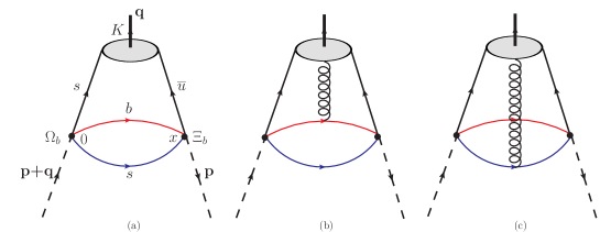
Figure 1: Contributions to $\Pi^{\mathrm{OPE}}(p,q)$ determined by two-particle (a), and three-particle distribution amplitudes of $K$ meson (b) and (c).

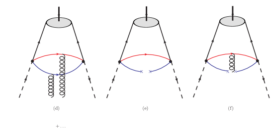
Figure 2: Diagrams with gluon (a), quark (b), and mixed (c) vacuum condensates.

The sum rules for the strong couplings can be derived after continuum subtraction. There are two known approaches to perform this procedure. Thus, in the context of the first method one calculates a double spectral density $\rho^{\mathrm{OPE}}(s_{1},\,s_{2})$ as an imaginary part of the correlation function, and using ideas of the quark-hadron duality carries out subtraction. In the second approach it is necessary to get spectral density $\rho(s_{1},\,s_{2})$ directly from Borel transformation of the correlation function in accordance with prescriptions developed in Refs. Ball:1994 ; Belyaev:1994zk ; Aliev:2010yx ; Aliev:2011ufa . In this approach for $M_{1}^{2}=M_{2}^{2}=2M^{2}$ and $u_{0}=1/2$ (see, text below) the continuum subtraction can be done using simple operations. For example, in the Borel transformation of the correlation function terms

$$\left(M^{2}\right)^{N}e^{-m^{2}/M^{2}}$$ (14)

preserve their original form if $N\leq 0$, and should be replaced by

$$\left(M^{2}\right)^{N}e^{-m^{2}/M^{2}}\rightarrow\frac{1}{\Gamma(N)}\int_{m^{2}}^{s_{0}}dse^{-s/M^{2}}\left(s-m^{2}\right)^{N-1},$$ (15)

if $N>0$. The subtracted version of other expressions, which emerge in calculations are collected in the Appendix A. In the present work to perform the continuum subtraction we follow these procedures.

To derive the sum rules for the strong couplings it is possible to use different Lorentz structures in Eq. (13). We have found that structures $\sim\not{q}\not{p}\gamma_{5}$ and $\sim\not{p}\gamma_{5}$ are convenient for our purposes. Isolating the corresponding terms in the Borel transformed form of the correlation function $\Pi^{\mathrm{OPE}}(p,\,q)$ we obtain:

$$g_{\widetilde{\Omega}_{b}\Xi_{b}K}=\frac{e^{\widetilde{m}^{2}/M_{1}^{2}}e^{m_{\Xi_{b}}^{2}/M_{2}^{2}}}{\lambda_{\Xi_{b}}\widetilde{\lambda}(m^{\prime}+\widetilde{m})}\left[(m^{\prime}-m_{\Xi_{b}})\mathcal{B}\Pi_{1}^{\mathrm{OPE}}-\mathcal{B}\Pi_{2}^{\mathrm{OPE}}\right],$$ (16)

and

$$g_{\Omega_{b}^{\prime}\Xi_{b}K}=\frac{e^{m^{\prime 2}/M_{1}^{2}}e^{m_{\Xi_{b}}^{2}/M_{2}^{2}}}{\lambda_{\Xi_{b}}\lambda^{\prime}(m^{\prime}+\widetilde{m})}\left[(\widetilde{m}+m_{\Xi_{b}})\mathcal{B}\Pi_{1}^{\mathrm{OPE}}+\mathcal{B}\Pi_{2}^{\mathrm{OPE}}\right],$$ (17)

where $\Pi_{1}^{\mathrm{OPE}}(p^{2},\,p^{\prime 2})$ and $\Pi_{2}^{\mathrm{OPE}}(p^{2},\,p^{\prime 2})$ are the invariant amplitudes corresponding to the structures $\not{q}\not{p}\gamma_{5}$ and $\not{p}\gamma_{5}$, respectively.

Because the masses of the initial $\Omega_{b}$ and final $\Xi_{b}^{0}$ baryons are close to each other we choose $M_{1}^{2}=M_{2}^{2}$, and introduce the Borel parameter $M^{2}$ through the equality

$$\frac{1}{M^{2}}=\frac{1}{M_{1}^{2}}+\frac{1}{M_{2}^{2}},$$ (18)

which simplifies considerably the obtained expressions. In the Appendix we write down the full expression for $\mathcal{B}\Pi_{1}^{\mathrm{OPE}}=$ $\Pi_{1}(M^{2})$ in terms of $K$-meson’s DAs. Some of $K$ meson DAs and values of corresponding parameters are also collected there.

Using the couplings $g_{\widetilde{\Omega}_{b}\Xi_{b}K}$ and $g_{\Omega_{b}^{\prime}\Xi_{b}K}$ it is not difficult to calculate the width of $\widetilde{\Omega}_{b}^{-}\rightarrow\Xi_{b}^{0}K^{-}$ and $\Omega_{b}^{\prime-}\rightarrow\Xi_{b}^{0}K^{-}$ decays. The required expressions are presented below:

$$\Gamma\left(\widetilde{\Omega}_{b}\rightarrow\Xi_{b}^{0}K^{-}\right) = \frac{g_{\widetilde{\Omega}_{b}\Xi_{b}K}^{2}}{8\pi\widetilde{m}^{2}}\left[(\widetilde{m}+m_{\Xi_{b}})^{2}-m_{K}^{2}\right]$$ (19)

$$\times f(\widetilde{m},m_{\Xi_{b}},m_{K}).$$

and

$$\Gamma\left(\Omega_{b}^{\prime}\rightarrow\Xi_{b}^{0}K^{-}\right) = \frac{g_{\Omega_{b}^{\prime}\Xi_{b}K}^{2}}{8\pi m^{\prime 2}}\left[(m^{\prime}-m_{\Xi_{b}})^{2}-m_{K}^{2}\right]$$ (20)

$$\times f(m^{\prime},m_{\Xi_{b}},m_{K}),$$

In expressions above the function $f(x,y,z)$ is given as:

$$f(x,y,z)=\frac{1}{2x}\sqrt{x^{4}+y^{4}+z^{4}-2x^{2}y^{2}-2x^{2}z^{2}-2y^{2}z^{2}}.$$

II.2 Decays $\widetilde{\Omega}_{b}^{\star}\to\Xi_{b}^{0}K^{-}$ and $\Omega_{b}^{\star\prime}\to\Xi_{b}^{0}K^{-}$

The decays of the spin-$3/2$ baryons $\widetilde{\Omega}_{b}^{\star}$ and $\Omega_{b}^{\star\prime}$ to $\Xi_{b}^{0}\,K^{-}$ can be analyzed as it has been done in previous subsection for the spin-$1/2$ baryons. To this end, we consider the correlation function

$$\Pi_{\mu}(p,q)=i\int d^{4}xe^{ipx}\langle K(q)|\mathcal{T}\{\eta_{\Xi_{b}}(x)\overline{\eta}_{\mu}(0)\}|0\rangle,$$ (21)

where the interpolating current $\eta_{\mu}(x)$ is given in the form

$$\eta_{\mu}=\frac{1}{\sqrt{3}}\epsilon^{abc}\left[\left(s^{aT}C\gamma_{\mu}s^{b}\right)b^{c}+2\left(s^{aT}C\gamma_{\mu}b^{b}\right)s^{c}\right].$$ (22)

In order to express the function $\Pi_{\mu}(p,q)$ in terms of the physical parameters of the involved particles we follow the same manipulations as in the case of the spin-1/2 baryons, the difference being only in definitions of the relevant matrix elements. Thus, we employ the following matrix elements for the spin-3/2 baryons

$$\langle 0|\eta_{\mu}|\widetilde{\Omega}_{b}^{\star}(p,s)\rangle = \widetilde{\lambda}^{\star}\gamma_{5}\widetilde{u}_{\mu}(p,s),$$

$$\langle 0|\eta_{\mu}|\Omega_{b}^{\star\prime}(p,s)\rangle = \lambda^{\star\prime}u_{\mu}^{\prime}(p,s),$$ (23)

where $u_{\mu}(p,s)$ are Rarita-Schwinger spinors, and $\widetilde{\lambda}^{\star}$ and $\lambda^{\star\prime}$ are residues of the $\widetilde{\Omega}_{b}^{\star}$ and $\Omega_{b}^{\star\prime}$ baryons, respectively.

We introduce also the strong couplings $g_{\widetilde{\Omega}_{b}^{\star}\Xi_{b}K}$ and $g_{\Omega_{b}^{\star\prime}\Xi_{b}K}$ by means of the formulas

$$\langle K(q)\Xi_{b}^{0}(p,s)|\widetilde{\Omega}_{b}^{\star}(p^{\prime},s^{\prime})\rangle=g_{\widetilde{\Omega}_{b}^{\star}\Xi_{b}K}\overline{u}(p,s)\gamma_{5}u_{\alpha}(p^{\prime},s^{\prime})q^{\alpha},$$

$$\langle K(q)\Xi_{b}^{0}(p,s)|\Omega_{b}^{\star\prime}(p^{\prime},s^{\prime})\rangle=g_{\Omega_{b}^{\star\prime}\Xi_{b}K}\overline{u}(p,s)u_{\alpha}(p^{\prime},s^{\prime})q^{\alpha}.$$

Substituting the matrix elements given by Eqs. (23) and (LABEL:eq:MElem3) into $\Pi_{\mu}^{\mathrm{Phys}}(p,q)$ and performing the summation over the spins in accordance with the expression

$$\sum\limits_{s}u_{\mu}(p,s)\overline{u}_{\nu}(p,s)=-(\not{p}+m)\left[g_{\mu\nu}-\frac{1}{3}\gamma_{\mu}\gamma_{\nu}\right.$$

$$\left.-\frac{2}{3m^{2}}p_{\mu}p_{\nu}+\frac{1}{3m}(p_{\mu}\gamma_{\nu}-p_{\nu}\gamma_{\mu})\right],$$ (25)

we get

$$\Pi_{\mu}^{\mathrm{Phys}}(p,q)=\frac{g_{\widetilde{\Omega}_{b}^{\star}\Xi_{b}K}\lambda_{\Xi_{b}}\widetilde{\lambda}^{\star}}{(p^{2}-m_{\Xi_{b}}^{2})(p^{\prime}{}^{2}-\widetilde{m}^{\star 2})}q^{\alpha}(\not{p}+m_{\Xi_{b}})\gamma_{5}$$

$$\times\left(\not{p}+\not{q}+\widetilde{m}^{\star}\right)F_{\alpha\mu}(\widetilde{m}^{\star})\gamma_{5}$$

$$-\frac{g_{\Omega_{b}^{\star\prime}\Xi_{b}K}\lambda_{\Xi_{b}}\lambda^{\ast\prime}}{(p^{2}-m_{\Xi_{c}}^{2})(p^{\prime 2}-m^{\prime 2})}q^{\alpha}(\not{p}+m_{\Xi_{b}})$$

$$\times\left(\not{p}+\not{q}+m^{\ast\prime}\right)F_{\alpha\mu}(m^{\ast\prime})+\ldots.$$ (26)

In Eq. (26) we have used the notation

$$F_{\alpha\mu}(m)=g_{\alpha\mu}-\frac{1}{3}\gamma_{\alpha}\gamma_{\mu}-\frac{2}{3m^{2}}(p_{\alpha}+q_{\alpha})(p_{\mu}+q_{\mu})$$

$$+\frac{1}{3m}\left[(p_{\alpha}+q_{\alpha})\gamma_{\mu}-(p_{\mu}+q_{\mu})\gamma_{\alpha}\right].$$ (27)

For the Borel transformation of $\Pi_{\mu}^{\mathrm{Phys}}(p,q)$ we obtain

$$\mathcal{B}\Pi_{\mu}^{\mathrm{Phys}}(p,q)=g_{\widetilde{\Omega}_{b}^{\star}\Xi_{b}K}\lambda_{\Xi_{b}}\widetilde{\lambda}e^{-\widetilde{m}^{2}/M_{1}^{2}}e^{-m_{\Xi_{b}}^{2}/M_{2}^{2}}q^{\alpha}$$

$$\times(\not{p}+m_{\Xi_{b}})\gamma_{5}\left(\not{p}+\not{q}+\widetilde{m}^{\star}\right)F_{\alpha\mu}(\widetilde{m}^{\star})\gamma_{5}$$

$$-g_{\Omega_{b}^{\star\prime}\Xi_{b}K}\lambda_{\Xi_{b}}\lambda^{\star\prime}e^{-m^{\prime 2}/M_{1}^{2}}e^{-m_{\Xi_{b}}^{2}/M_{2}^{2}}q^{\alpha}(\not{p}+m_{\Xi_{b}})$$

$$\times\left(\not{p}+\not{q}+m^{\star\prime}\right)F_{\alpha\mu}(m^{\star\prime}).$$ (28)

The required sum rules can be obtained by using invariant amplitudes corresponding to the structures $\not{q}\not{p}\gamma_{\mu}$ and $\not{q}q_{\mu}$.

The correlation function $\Pi_{\mu}^{\mathrm{OPE}}(p,q)$ is determined in terms of numerous distribution amplitudes of the $K$ meson. In Appendix we also provide the explicit expression for double Borel transformed form of the invariant amplitude corresponding to the structure $\not{q}\not{p}\gamma_{\mu}$ . By fixing the same structures in both $\mathcal{B}\Pi_{\mu}^{\mathrm{Phys}}(p,q)$ and $\mathcal{B}\Pi_{\mu}^{\mathrm{OPE}}(p,q)$ and equating Borel transformed form of the relevant invariant amplitudes, it is possible to get and solve two equations for the strong couplings $g_{\widetilde{\Omega}_{b}^{\star}\Xi_{b}K}$ and $g_{\Omega_{b}^{\star\prime}\Xi_{b}K}$.

Then the width of the $\widetilde{\Omega}_{b}^{\star}\rightarrow\Xi_{b}^{0}K^{-}$ decay can be obtained as

$$\Gamma(\widetilde{\Omega}_{b}^{\star} \rightarrow \Xi_{b}^{0}K^{-})=\frac{g_{\widetilde{\Omega}_{b}^{\star}\Xi_{b}K}^{2}}{24\pi\widetilde{m}^{\star 2}}\left[(\widetilde{m}^{\star}-m_{\Xi_{b}})^{2}-m_{K}^{2}\right]$$ (29)

$$\times f^{3}(\widetilde{m}^{\star},m_{\Xi_{b}},m_{K}),$$

whereas for $\Gamma(\Omega_{c}^{\star\prime}\rightarrow\Xi_{b}^{0}K^{-})$ we find

$$\Gamma(\Omega_{b}^{\star\prime} \rightarrow \Xi_{b}^{0}K^{-})=\frac{g_{\Omega_{b}^{\star\prime}\Xi_{b}K}^{2}}{24\pi m^{\star\prime 2}}\left[(m^{\star\prime}+m_{\Xi_{b}})^{2}-m_{K}^{2}\right]$$ (30)

$$\times f^{3}(m^{\star\prime},m_{\Xi_{b}},m_{K}).$$

These expressions will be used in numerical calculations.

III Numerical computations

The obtained sum rules for the strong couplings depend on numerous parameters. First of all, the light-cone propagator of $s-$quark contains the quark and mixed vacuum condensates numerical value of which $\langle\overline{s}s\rangle=-0.8\times(0.24\pm 0.01)^{3}~{}\mathrm{GeV}^{3}$, $\langle\overline{s}g_{s}\sigma Gs\rangle=m_{0}^{2}\langle\overline{s}s\rangle$, where $m_{0}^{2}=(0.8\pm 0.1)~{}\mathrm{GeV}^{2}$ are well known. For the gluon condensate we utilize $\langle\alpha_{s}G^{2}/\pi\rangle=(0.012\pm 0.004)~{}\mathrm{GeV}^{4}$. The masses of the $b-$ and $s$-quarks are presented in PDG Olive:2016xmw : $m_{b}=4.18_{-0.03}^{+0.04}~{}\mathrm{GeV}$ and $m_{s}=96_{-4}^{+8}~{}\mathrm{MeV}$. The residue $\lambda_{\Xi_{b}}=0.054\pm 0.012$ $\mathrm{GeV}^{3}$ of $\Xi_{b}^{0}$ baryon is borrowed from Ref. Azizi:2016dmr .

Calculations within the sum rule method imply fixing of the working windows for the Borel parameter $M^{2}$ and continuum threshold $s_{0}$, which are two auxiliary parameters of computations. In addition, formulas for the spin-$1/2$ baryons depend on $\beta$ arising from the expressions of the interpolating currents $\eta(x)$ and $\eta_{\Xi_{b}}(x)$. The mass and pole residue of the excited bottom baryons also appear in the sum rules for the strong couplings as input parameters. In our previous work Agaev:2017jyt we evaluated the spectroscopic parameters of the $\widetilde{\Omega}_{b}$, $\Omega_{b}^{\prime}$ and $\widetilde{\Omega}_{b}^{\star}$, $\Omega_{b}^{\star\prime}$ baryons. Predictions obtained there for the mass and pole residue of $1P$ and $2S$ bottom baryons with $J=1/2$ and $J=3/2$, as well as the working ranges of the parameters $M^{2}$ and $s_{0}$ are collected in Table 1. Results for the spin-$1/2$ baryons were extracted by varying the parameter $\beta=\tan\theta$ in Eq. (6) within the limits

$$-0.75\leq\cos\theta\leq-0.45,\ 0.45\leq\cos\theta\leq 0.75,$$ (31)

which led to stable predictions for their masses and residues.

The choice of $M^{2}$, $s_{0}$ and $\beta$ is not arbitrary, but has to satisfy restrictions of sum rule calculations. Thus, the upper bound of the working region for $M^{2}$ is obtained from the constraint imposed on the pole contribution

$$\frac{\Pi^{\mathrm{OPE}}(M^{2},\ s_{0},\ \beta)}{\Pi^{\mathrm{OPE}}(M^{2},\ \infty,\ \beta)}>\frac{1}{2},$$ (32)

where $\Pi^{\mathrm{OPE}}(M^{2},\ s_{0},\ \beta)$ is the Borel transformation of the relevant correlation function after continuum subtraction.

The lower limit of the Borel parameter $M^{2}$ is determined from exceeding of the perturbative contribution over the nonperturbative one as well as convergence of the operator product expansion. In the present work we apply the following criteria: at the lower bound of the Borel window the perturbative contribution has to constitute $\geq 80\%$ part of the corresponding sum rule, and contribution of the highest dimensional term (i.e., in our case $\mathrm{Dim}9$ term ) should not exceed $1\%$ of the whole result.

The limits within of which the parameter $s_{0}$ can be varied are determined from the pole to total contribution ratio to achieve its greatest possible value. Quantities extracted from sum rules have also to demonstrate minimal dependence on $M^{2}$ while varying $s_{0}$ in the allowed domain.

$(n,J^{P})$	$(1P,\frac{1}{2}^{-})$	$(2S,\frac{1}{2}^{+})$	$(1P,\frac{3}{2}^{-})$	$(2S,\frac{3}{2}^{+})$
$M^{2}~{}(\mathrm{GeV}^{2}$)	$6.5-9.5$	$6.5-9.5$	$6.5-9.5$	$6.5-9.5$
$s_{0}~{}(\mathrm{GeV}^{2}$)	$6.6^{2}-6.8^{2}$	$6.8^{2}-7.0^{2}$	$6.7^{2}-6.9^{2}$	$6.9^{2}-7.1^{2}$
$m_{\Omega_{b}}~{}(\mathrm{MeV})$	$6336\pm 183$	$6487\pm 187$	$6301\pm 193$	$6422\pm 198$
$\lambda_{\Omega_{b}}\cdot 10^{2}~{}(\mathrm{GeV}^{3})$	$17.5\pm 2.9$	$19.8\pm 4.1$	$19.2\pm 3.1$	$29.1\pm 5.3$

Table 1: The $m_{\Omega_{b}}$ and $\lambda_{\Omega_{b}}$ of the excited bottom baryons with $J=1/2$ and $J=3/2$.

Finally, we determine a working range for $\beta$ by demanding a weak dependence of our results on its choice, which quantitatively reads

$$\frac{|\Pi^{\mathrm{OPE}}(M^{2},\ s_{0},\beta_{0})-\Pi^{\mathrm{OPE}}(M^{2},\ s_{0},\beta_{0}\pm\Delta\beta)|}{\Pi^{\mathrm{OPE}}(M^{2},\ s_{0},\ \beta_{0})}\leq 0.1,$$ (33)

where $\beta_{0}\pm\Delta\beta\in[\beta_{\mathrm{min}},\ \beta_{\mathrm{max}}]$.

In the choice of the regions for $M^{2}$, $s_{0}$, and $\beta$ we keep in mind that sum rules for masses and pole residues of the excited $\Omega_{b}$ baryons also depend on these parameters. Because they enter as input quantities to sum rules for the strong couplings a deviation from regions found in Ref. Agaev:2017jyt may generate additional uncertainties.

Analysis carried out in accordance with these requirements enables us to fix the parameters $M^{2}$, $s_{0}$ and $\beta$. Thus, for both the spin-1/2 and spin-3/2 bottom baryons the working region for the Borel parameter is

$$M^{2}\in[6.5-9.5]\ \mathrm{GeV}^{2}.$$

The regions for the continuum threshold $s_{0}$ depend on type of the $\Omega_{b}$ baryon under consideration. For calculation of the strong coupling of $1P$ and $2S$ excitations of the spin-1/2 baryon we use

$$s_{0} \in [6.6^{2}-6.8^{2}]\ \mathrm{GeV}^{2},$$

$$s_{0} \in [6.8^{2}-7.0^{2}]\ \mathrm{GeV}^{2},$$ (34)

respectively. For the same excited states of the spin-3/2 baryon we get

$$s_{0} \in [6.7^{2}-6.9^{2}]\ \mathrm{GeV}^{2},$$

$$s_{0} \in [6.9^{2}-7.1^{2}]\ \mathrm{GeV}^{2}.$$ (35)

For spin-1/2 particles the parameter $\beta$ is fixed as in Eq. (31).

In regions chosen for $M^{2}$, $s_{0}$ and $\beta$ the sum rules comply aforementioned constraints. Thus, in Fig. 3 we plot the pole contribution to the sum rule for $g_{\widetilde{\Omega}_{b}^{\star}\Xi_{b}K}$, which at $M^{2}=9.5\ \mathrm{GeV}^{2}$ equals to $64\%$ of the whole contribution, and reaches $75\%$ of its value in the case of $g_{\Omega_{b}^{\star\prime}\Xi_{b}K}$.

In Fig. 4 we compare the perturbative and nonperturbative contributions to the strong coupling $g_{\widetilde{\Omega}_{b}^{\star}\Xi_{b}K}$ as functions of $M^{2}$ and $s_{0}$ at central values of $s_{0}$ and $M^{2}$, respectively. It is seen, that the perturbative contribution amounts to more than $0.8$ part of the result. Convergence of OPE becomes evident from analysis of Fig. 5, where by the curve labelled $\geq\mathrm{Dim}6$ we depict the sum of nonperturbative terms from sixth till ninth dimensions. They already satisfy the imposed constraint on nonperturbative terms to guaranty convergence of the expansion.

Dependence on $\beta$ is mild: at the central values of $M^{2}=8$ $\mathrm{GeV}^{2}$ and $s_{0}=6.7^{2}\ \mathrm{GeV}^{2}$ variation of $\beta$ within limits determined by Eq. (31) leads only to $\sim 7\%$  changes in $g_{\widetilde{\Omega}_{b}\Xi_{b}K}$, whereas at $M^{2}=8$ $\mathrm{GeV}^{2}$ and $s_{0}=6.9^{2}\ \mathrm{GeV}^{2}$ they amount approximately to $8\%$ of $g_{\Omega_{b}^{\prime}\Xi_{b}K}$. In the whole region of $M^{2}$ and $s_{0}$ they do not overshoot $10\%$ of the results, and are in agreement with Eq. (33).

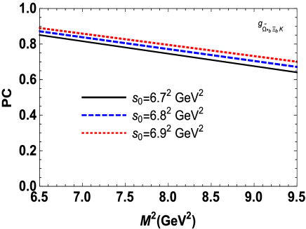
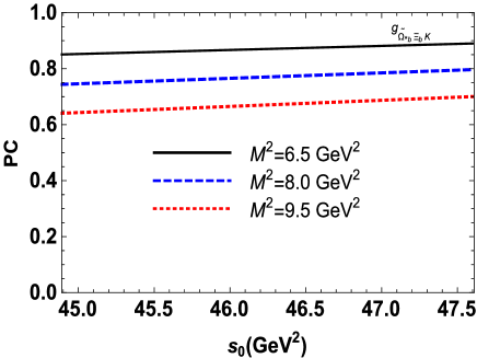
Figure 3: The dependence of the pole contribution to $g_{\widetilde{\Omega}_{b}^{\star}\Xi_{b}K}$ on the Borel parameter $M^{2}$ (left panel), and on the continuum threshold $s_{0}$ (right panel).

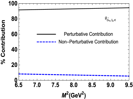
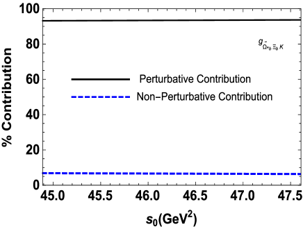
Figure 4: The perturbative and nonperturbative contributions to the coupling $g_{\widetilde{\Omega}_{b}^{\star}\Xi_{b}K}$ as functions of the Borel parameter $M^{2}$ (left panel), and of the continuum threshold $s_{0}$ (right panel).

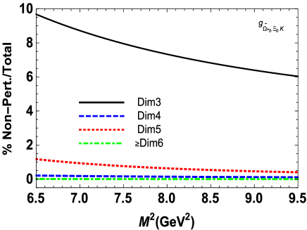
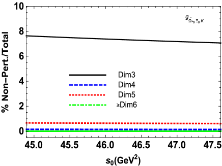
Figure 5: The nonperturbative contributions to the strong coupling $g_{\widetilde{\Omega}_{b}^{\star}\Xi_{b}K}$ as functions of the Borel parameter $M^{2}$ (at $s_{0}=46.25\ \mathrm{GeV}^{2}$, left panel), and of the continuum threshold $s_{0}$ ($M^{2}=8\ \mathrm{GeV}^{2}$, right panel).

The regions for $M^{2}$ and $s_{0}$ in the light-cone sum rule computations of the strong couplings $g_{\widetilde{\Omega}_{b}\Xi_{b}K}$, $\ g_{\Omega_{b}^{\prime}\Xi_{b}K}$ , $g_{\widetilde{\Omega}_{b}^{\star}\Xi_{b}K}$ and $g_{\Omega_{b}^{\star\prime}\Xi_{b}K}$ coincide with ones used in calculations of the mass and residue of $\widetilde{\Omega}_{b}$, $\Omega_{b}^{\prime}$, $\widetilde{\Omega}_{b}^{\star}$ and $\Omega_{b}^{\star\prime}$ baryons. By such choice of working windows for $M^{2}$, $s_{0}$ and $\beta$ we also evade appearance of additional theoretical uncertainties.

The strong couplings of the excited spin-1/2 $\Omega_{b}$ baryons equal to:

$$g_{\widetilde{\Omega}_{b}\Xi_{b}K}=0.36\pm 0.07,\ \ g_{\Omega_{b}^{\prime}\Xi_{b}K}=7.33\pm 1.61.\$$ (36)

For couplings of the $\Omega_{b}^{\star}$ baryons we get

$$g_{\widetilde{\Omega}_{b}^{\star}\Xi_{b}K}=82.29\pm 14.08,\ g_{\Omega_{b}^{\star\prime}\Xi_{b}K}=1.04\pm 0.28.\$$ (37)

Here we provide also theoretical errors of our predictions essential part of which comes from uncertainties in the choice of the auxiliary parameters $M^{2}$ and $s_{0}$ (for spin-1/2 baryons also from $\beta$). Theoretical errors vary from $\pm 15\%$  for $g_{\widetilde{\Omega}_{b}^{\star}\Xi_{b}K}$ till $\pm 27\%$ for $g_{\Omega_{b}^{\star\prime}\Xi_{b}K}$ and do not exceed $30\%$ of the central values, which is an accuracy accepted in QCD sum rule calculations. To demonstrate a sensitivity of the obtained results to choice of these parameters in Figs. 6, 7 and 8 we plot $g_{\Omega_{b}^{\prime}\Xi_{b}K}$, $g_{\widetilde{\Omega}_{b}^{\star}\Xi_{b}K}$ and $g_{\Omega_{b}^{\star\prime}\Xi_{b}K}$ as functions of $M^{2}$ at fixed $s_{0}$, and functions of $s_{0}$ for chosen $M^{2}$.

For width of the excited $1P$ and $2S$ bottom baryons’ decays we find: for $\Omega_{b}$

$$\Gamma\left(\widetilde{\Omega}_{b}\rightarrow\Xi_{b}^{0}K^{-}\right) = 3.97\pm 0.91\ \mathrm{MeV},\$$

$$\Gamma\left(\Omega_{b}^{\prime}\rightarrow\Xi_{b}^{0}K^{-}\right) = 5.51\pm 1.42\ \mathrm{MeV},$$ (38)

and for $\Omega_{b}^{\star}$

$$\ \Gamma(\widetilde{\Omega}_{b}^{\star} \rightarrow \Xi_{b}^{0}K^{-})=0.04\pm 0.01\ \mathrm{MeV},$$

$$\Gamma(\Omega_{b}^{\star\prime} \rightarrow \Xi_{b}^{0}K^{-})=2.57\pm 0.78\ \mathrm{MeV}.$$ (39)

The predictions for width of the decay processes given by Eqs. (38) and (39) are our final results.

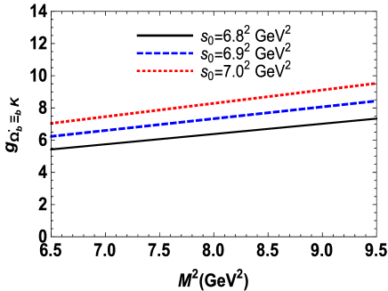
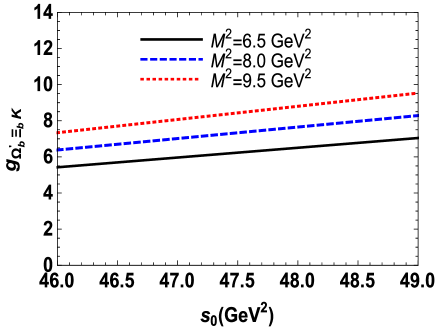
Figure 6: The dependence of the strong coupling $g_{\Omega_{b}^{\prime}\Xi_{b}K}$ on the Borel parameter $M^{2}$ at fixed $s_{0}$ (left panel), and on the continuum threshold $s_{0}$ for chosen $M^{2}$ (right panel).

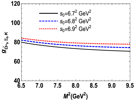
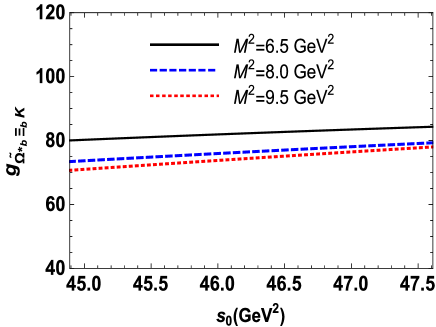
Figure 7: The strong coupling $g_{\widetilde{\Omega}_{b}^{\star}\Xi_{b}K}$ vs the Borel parameter $M^{2}$ (left panel), and vs continuum threshold $s_{0}$ (right panel).

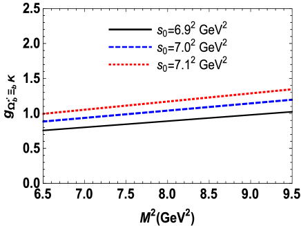
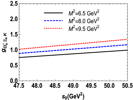
Figure 8: The strong coupling of the radially excited $\Omega_{b}^{\star\prime}$ baryon with $\Xi_{b}K$ as a function of the Borel parameter $M^{2}$ at fixed $s_{0}$ (left panel), and as a function of the continuum threshold $s_{0}$ at different $M^{2}$ (right panel).

IV Concluding remarks

In the present study we have investigated the decay processes involving the orbitally and radially excited spin-1/2 and spin-3/2 bottom baryons $\Omega_{b}$ and $\Omega_{b}^{\star}$, respectively. It is worth noting that the hadronic processes with heavy baryons and their excitations are interesting from theoretical point of view, but after discoveries of the LHCb Collaboration they are on agenda of the experimental collaborations, as well.

In our previous works Agaev:2017jyt ; Agaev:2017lip we have explained four of the recently discovered five narrow charmonium-like resonances as the first orbital and radial excitations of the spin-1/2 and spin-3/2 $\Omega_{c}$ and $\Omega_{c}^{\star}$ baryons. The masses of their bottom counterparts were already calculated in Ref. Agaev:2017jyt . The mass range of the bottom baryons obtained there indicates that the mass splitting between $(1P,1/2^{-})$ and $(1P,3/2^{-})$ baryons, and between $(2S,1/2^{+})$ and $(2S,3/2^{+})$ baryons is small. At the same time, there is a mass gap between $1P$ and $2S$ states, which may be occupied by ”fifth” resonance. In the present work we have computed the widths of the four $1P$ and $2S$ baryons’ decays to $\Xi_{b}^{0}K^{-}$. The obtained results may be useful for forthcoming experiments to explore the bottom baryons and measure their spectroscopic and dynamical parameters.

*

Appendix A The correlation functions and K meson DAs

In this Appendix we provide explicit expressions for double Borel transformed form of the invariant amplitude $\Pi_{1}(M^{2})$ for spin-1/2 baryons, as well as the double Borel transformed form of the invariant amplitude corresponding to the structure $\not{q}\not{p}\gamma_{\mu}$ in the correlation function of the spin-3/2 baryons.

For $\Pi_{1}(M^{2})$ we get:

$$\Pi_{1}(M^{2})=\Pi^{\mathrm{I}}(M^{2})+\Pi^{\mathrm{\langle s\bar{s}\rangle}}(M^{2})+\Pi^{\mathrm{\langle GG\rangle}}(M^{2})+\Pi^{\mathrm{\langle sG\bar{s}\rangle}}(M^{2})+\Pi^{\mathrm{\langle s\bar{s}\rangle\langle GG\rangle}}(M^{2})+\Pi^{\mathrm{\langle sG\bar{s}\rangle\langle GG\rangle}}(M^{2}),$$ (A.40)

$$\Pi^{\mathrm{I}}(M^{2}) = \frac{1}{96\sqrt{2}\pi^{2}}\int_{m_{b}^{2}}^{\infty}dse^{\frac{m_{K}^{2}-4s}{4M^{2}}}\frac{m_{b}}{s^{3}}\Bigg{\{}\sqrt{3}m_{b}^{2}M^{2}\Bigg{[}3f_{K}m_{K}^{2}(1-\beta^{2})s\mathbb{A}(u_{0})-12f_{K}M^{2}(1-\beta)\Big{[}(1+\beta)(s-m_{b}^{2})$$ (A.41)

$$+ \beta m_{b}m_{s}\Big{]}\phi_{K}(u_{0})-4\mu_{K}(\widetilde{\mu}_{K}^{2}-1)\Big{[}(\beta-1)(2\beta+1)M^{2}m_{b}+2(1+\beta+\beta^{2})sm_{s}\Big{]}\phi_{\sigma}(u_{0})\Bigg{]}+f_{K}m_{K}^{2}(\beta-1)$$

$$+ \Bigg{(}M^{2}\Big{[}(\beta-1)s^{2}+2\beta sm_{b}m_{s}+(3+\beta)sm_{b}^{2}-(\beta-1)m_{b}^{3}m_{s}\Big{]}+(\beta-1)m_{b}^{3}m_{s}(s+2M^{2})\mathrm{Ln}[\Psi]\Bigg{)}$$

$$\times I_{1}\Big{(}\mathcal{A}_{\parallel}(\alpha),1\Big{)}+2f_{K}m_{K}^{2}(\beta-1)(1+3\beta)\Bigg{(}M^{2}\Big{[}m_{b}^{3}m_{s}+sm_{b}(2m_{b}-m_{s})-s^{2}\Big{]}+m_{b}^{3}m_{s}(2M^{2}+s)\mathrm{Ln}[\Psi]\Bigg{)}$$

$$\times I_{1}\Big{(}\mathcal{A}_{\perp}(\alpha),1\Big{)}+2f_{K}m_{K}m_{b}(\beta-1)\Bigg{(}M^{2}\Big{[}sm_{s}+sm_{b}(1+\beta)+m_{b}^{2}m_{s}(1+2\beta)\Big{]}+(1+2\beta)(s+2M^{2})m_{b}^{2}$$

$$\times m_{s}\mathrm{Ln}[\Psi]\Bigg{)}I_{1}\Big{(}\mathcal{V}_{\parallel}(\alpha),1\Big{)}+2f_{K}m_{K}^{2}(\beta-1)\Bigg{(}M^{2}\Big{[}2\beta mb^{3}m_{s}+2(1+2\beta^{2})s+(3+\beta)sm_{b}m_{s}-(5+3\beta)sm_{b}^{2}\Big{]}$$

$$+ 2\beta(s+2M^{2})m_{b}^{3}m_{s}\mathrm{Ln}[\Psi]\Bigg{)}I_{1}\Big{(}\mathcal{V}_{\perp}(\alpha),1\Big{)}+4(\beta-1)\mu_{K}M^{2}m_{K}^{2}m_{b}\Big{[}4mb^{2}(1+2\beta)-3s(1+\beta)\Big{]}I_{1}\Big{(}\mathcal{T}(\alpha),1\Big{)}$$

$$+ 4(\beta-1)f_{K}m_{K}^{2}M^{2}m_{b}s[(1+\beta)m_{b}+\beta m_{s}]I_{1}\Big{(}\mathcal{A}_{\parallel}(\alpha),v\Big{)}+4(1-\beta)(3+\beta)sf_{K}m_{K}^{2}M^{2}m_{b}(m_{b}-m_{s})$$

$$\times I_{1}\Big{(}\mathcal{V}_{\perp}(\alpha),v\Big{)}+18(\beta-1)\mu_{K}M^{2}m_{K}^{2}m_{b}[m_{b}^{2}(1+\beta)-s]u_{0}I_{1}\Big{(}\mathcal{T}(\alpha),v\Big{)}+(\beta-1)\mu_{K}M^{4}m_{b}$$

$$\times [4m_{b}^{2}(1+2\beta)-3s(1+\beta)]I_{2}\Big{(}\mathcal{T}(\alpha),1\Big{)}-4(1-\beta)\mu_{K}M^{4}m_{b}[m_{b}^{2}(1+\beta)-s]I_{2}\Big{(}\mathcal{T}(\alpha),v\Big{)}\Bigg{\}}$$

$$+ \dfrac{(1-\beta)}{32\sqrt{6}\pi^{2}}e^{\dfrac{m_{K}^{2}-4m_{b}^{2}}{4M^{2}}}f_{K}m_{K}^{2}M^{2}m_{s}\Bigg{\{}t\mathbb{A}(u_{0})+\gamma_{E}\Bigg{[}(1-\beta)I_{1}\Big{(}\mathcal{A}_{\parallel}(\alpha),1\Big{)}+2(1+3\beta)I_{1}\Big{(}\mathcal{A}_{\perp}(\alpha),1\Big{)}$$

$$+ 2(1+2\beta)I_{1}\Big{(}\mathcal{V}_{\parallel}(\alpha),1\Big{)}-4\beta I_{1}\Big{(}\mathcal{V}_{\perp}(\alpha),1\Big{)}\Bigg{]}\Bigg{\}},$$

$$\Pi^{\mathrm{\langle s\bar{s}\rangle}}(M^{2}) = \dfrac{\langle s\bar{s}\rangle}{144\sqrt{6}M^{4}}e^{\dfrac{m_{K}^{2}-4m_{b}^{2}}{4M^{2}}}\Bigg{\{}3f_{K}m_{K}^{2}(\beta-1)\Big{[}m_{b}^{3}m_{s}(1+\beta)-2\beta M^{2}(m_{b}^{2}-M^{2})\Big{]}\mathbb{A}(u_{0})+12M^{2}(\beta-1)f_{K}$$ (A.42)

$$\times M^{2}\Big{(}m_{b}m_{s}(1+\beta)-2\beta M^{2}\Big{)}\phi_{K}(u_{0})-4M^{2}\mu_{K}(1-\tilde{\mu}_{K}^{2})\Bigg{(}4M^{2}m_{b}(1+\beta+\beta^{2})+m_{b}^{2}m_{s}(1+\beta-2\beta^{2})$$

$$- M^{2}m_{s}(1+\beta-2\beta^{2})\Bigg{)}\phi_{\sigma}(u_{0})+3M^{2}(\beta-1)f_{K}m_{K}^{2}\Bigg{[}\Big{(}m_{b}m_{s}(\beta-1)-4\beta M^{2}\Big{)}I_{1}\Big{(}\mathcal{A}_{\parallel}(\alpha),1\Big{)}+8\beta M^{2}$$

$$\times I_{1}\Big{(}\mathcal{A}_{\parallel}(\alpha),v\Big{)}-2(1+3\beta)(m_{b}m_{s}-2M^{2})I_{1}\Big{(}\mathcal{A}_{\perp}(\alpha),1\Big{)}-4\Big{(}m_{b}m_{s}(1+\beta)-M^{2}(3+\beta)\Big{)}I_{1}\Big{(}\mathcal{V}_{\perp}(\alpha),1\Big{)}$$

$$- 8(3+\beta)M^{2}I_{1}\Big{(}\mathcal{V}_{\perp}(\alpha),v\Big{)}-4M^{2}I_{1}\Big{(}\mathcal{V}_{\parallel}(\alpha),1\Big{)}\Bigg{]}-3M^{2}(\beta-1)\mu_{K}\Bigg{[}16m_{s}m_{K}^{2}u_{0}I_{1}\Big{(}\mathcal{T}(\alpha),v\Big{)}$$

$$- 12m_{K}^{2}m_{s}(1+\beta)u_{0}I_{1}\Big{(}\mathcal{T}(\alpha),1\Big{)}-3M^{2}m_{s}(1+\beta)I_{2}\Big{(}\mathcal{T}(\alpha),1\Big{)}+4M^{2}m_{s}I_{2}\Big{(}\mathcal{T}(\alpha),v\Big{)}\Bigg{]}\Bigg{\}},$$

$$\Pi^{\mathrm{\langle GG\rangle}}(M^{2}) = \dfrac{\langle GG\rangle}{6912\sqrt{6}\pi^{2}M^{8}}\Bigg{\{}\int_{m_{b}^{2}}^{\infty}dse^{\frac{m_{K}^{2}-4s}{4M^{2}}}\Bigg{\{}\dfrac{3m_{b}}{s^{3}}\Bigg{[}3\beta(\beta-1)f_{K}m_{K}^{2}m_{b}^{3}m_{s}\Big{(}M^{2}(2M^{4}+3M^{2}s+3s^{2})+s^{3}\mathrm{Ln}[\Psi]\Big{)}\mathbb{A}(u_{0})$$ (A.43)

$$+ 12(\beta-1)M^{4}f_{K}\Big{[}M^{6}s+\beta M^{2}\Big{(}M^{4}s-m_{b}^{3}m_{s}(3M^{2}+2s)\Big{)}-\beta(2M^{4}+2M^{2}s+s^{2})m_{b}^{3}m_{s}\mathrm{Ln}[\Psi]\Big{]}\phi_{K}(u_{0})$$

$$- 8(1+\beta+\beta^{2})\mu_{K}(1-\tilde{\mu}_{K}^{2})M^{2}m_{b}^{2}m_{s}s\Big{[}M^{2}(M^{2}+2s)+s^{2}\mathrm{Ln}[\Psi]\Big{]}\phi_{\sigma}(u_{0})\Bigg{]}-\dfrac{3M^{2}}{s^{2}}(\beta-1)f_{K}m_{K}^{2}m_{b}^{2}m_{s}$$

$$\times \Big{(}M^{2}(M^{2}+2s)+s^{2}\mathrm{Ln}[\Psi]\Big{)}\Bigg{[}(1+5\beta)I_{1}\Big{(}\mathcal{A}_{\parallel}(\alpha),1\Big{)}-4I_{1}\Big{(}\mathcal{A}_{\perp}(\alpha),1\Big{)}-12\beta\Big{(}I_{1}\Big{(}\mathcal{A}_{\parallel}(\alpha),v\Big{)}$$

$$+ I_{1}\Big{(}\mathcal{A}_{\perp}(\alpha),1\Big{)}\Big{)}+4(2+\beta)I_{1}\Big{(}\mathcal{V}_{\parallel}(\alpha),1\Big{)}-2(9+5\beta)I_{1}\Big{(}\mathcal{V}_{\perp}(\alpha),1\Big{)}+12(3+\beta)I_{1}\Big{(}\mathcal{V}_{\perp}(\alpha),v\Big{)}\Bigg{]}\Bigg{\}}$$

$$+ e^{\frac{m_{K}^{2}-4m_{b}^{2}}{4M^{2}}}\Bigg{\{}\dfrac{M^{2}}{m_{b}}\Bigg{[}3(1-\beta)f_{K}m_{K}^{2}\Big{[}\beta(3\gamma_{E}-2)m_{b}^{5}m_{s}-\beta M^{2}m_{b}^{3}m_{s}-(1+\beta)M^{4}m_{b}^{2}+2(1+\beta)M^{6}\Big{]}\mathbb{A}(u_{0})$$

$$+ 12(1-\beta)f_{K}M^{4}\Big{[}\beta(2-3\gamma_{E})m_{b}^{3}m_{s}+M^{2}\Big{(}M^{2}+\beta(3(1-\gamma_{E})m_{b}m_{s}+M^{2})\Big{)}\Big{]}\phi_{K}(u_{0})+4\mu_{K}(1-\tilde{\mu}_{K}^{2})M^{2}$$

$$\times \Big{[}(1+\beta-2\beta^{2})M^{4}m_{b}+2(1+\beta+\beta^{2})\Big{(}m_{b}^{2}m_{s}((3\gamma_{E}-2)m_{b}^{2}-M^{2})+2M^{4}m_{s}\Big{)}\Big{]}\phi_{\sigma}(u_{0})\Bigg{]}$$

$$+ \dfrac{3M^{4}}{m_{b}}(\beta-1)f_{K}m_{K}^{2}\Bigg{[}\Big{(}(1+5\beta)\gamma_{E}m_{b}^{3}m_{s}-4\beta m_{b}^{3}m_{s}-2(1+\beta)M^{2}m_{b}^{2}+4(1+\beta)M^{4}\Big{)}I_{1}\Big{(}\mathcal{A}_{\parallel}(\alpha),1\Big{)}$$

$$- 2(1+3\beta)\Big{(}2(\gamma_{E}-1)m_{b}^{3}m_{s}+M^{2}m_{b}^{2}-2M^{4}\Big{)}I_{1}\Big{(}\mathcal{A}_{\perp}(\alpha),1\Big{)}+2\Big{(}(1+\beta)M^{2}(2M^{2}-m_{b}^{2})+2m_{b}^{3}m_{s}$$

$$\times (\gamma_{E}(2+\beta)-1)\Big{)}I_{1}\Big{(}\mathcal{V}_{\parallel}(\alpha),1\Big{)}-2\Big{(}(3+\beta)M^{2}(m_{b}^{2}-2M^{2})+m_{b}^{3}m_{s}(\gamma_{E}(9+5\beta)-3\beta-6)\Big{)}$$

$$\times I_{1}\Big{(}\mathcal{V}_{\perp}(\alpha),1\Big{)}+4(3+\beta)\Big{(}(3\gamma_{E}-2)m_{b}^{3}m_{s}+M^{2}(m_{b}^{2}-2M^{2})\Big{)}I_{1}\Big{(}\mathcal{V}_{\perp}(\alpha),v\Big{)}+4\Big{(}\beta(2-3\gamma_{E})m_{b}^{3}m_{s}$$

$$+ M^{2}(1+\beta)(m_{b}^{2}-2M^{2})\Big{)}I_{1}\Big{(}\mathcal{A}_{\parallel}(\alpha),v\Big{)}\Bigg{]}+\dfrac{3M^{4}}{m_{b}}(\beta-1)\mu_{K}\Bigg{[}4(1+5\beta)m_{K}^{2}M^{2}m_{b}u_{0}I_{1}\Big{(}\mathcal{T}(\alpha),1\Big{)}$$

$$- 16\beta m_{K}^{2}M^{2}m_{b}u_{0}I_{1}\Big{(}\mathcal{T}(\alpha),v\Big{)}+(1+5\beta)M^{4}m_{b}I_{2}\Big{(}\mathcal{T}(\alpha),1\Big{)}-4\beta M^{4}m_{b}I_{2}\Big{(}\mathcal{T}(\alpha),v\Big{)}\Bigg{]}\Bigg{\}}\Bigg{\}},$$

$$\Pi^{\mathrm{\langle sG\bar{s}\rangle}}(M^{2}) = \dfrac{m_{0}^{2}\langle s\bar{s}\rangle}{3456\sqrt{6}M^{8}}e^{\dfrac{m_{K}^{2}-4m_{b}^{2}}{4M^{2}}}\Bigg{\{}3f_{K}m_{K}^{2}m_{b}(\beta-1)\Big{[}4m_{b}^{2}m_{s}(1+\beta)(m_{b}^{2}-3M^{2})-12\beta m_{b}^{3}M^{2}+4M^{4}m_{s}$$ (A.44)

$$\times (1+\beta)+M^{4}m_{b}\Big{(}t-11+2(7+\beta)v\Big{)}\Big{]}\mathbb{A}(u_{0})+12(\beta-1)f_{K}M^{4}\Big{(}4m_{b}m_{s}(1+\beta)(m_{b}^{2}-M^{2})$$

$$+ M^{4}(2v(7+\beta)-11(1+\beta))\Big{)}\phi_{K}(u_{0})+8M^{2}\mu_{K}(\tilde{\mu}_{K}^{2})m_{b}\Big{[}2(2\beta+1)(\beta-1)m_{b}^{3}m_{s}+(4+\beta-5\beta^{2})$$

$$\times M^{2}m_{b}m_{s}-12(1+\beta+\beta^{2})M^{2}m_{b}^{2}+3M^{4}(3+2\beta+3\beta^{2})\Big{]}\phi_{\sigma}+12M^{2}(1-\beta)f_{K}m_{K}^{2}\Bigg{[}\Big{(}m_{s}(\beta-1)$$

$$\times (m_{b}^{2}-M^{2})-6\beta M^{2}m_{b}\Big{)}I_{1}\Big{(}\mathcal{A}_{\parallel}(\alpha),1\Big{)}+12\beta M^{2}m_{b}I_{1}\Big{(}\mathcal{A}_{\parallel}(\alpha),v\Big{)}+2(1+3\beta)\Big{(}M^{2}(3m_{b}+m_{s})$$

$$- m_{b}^{2}m_{s}\Big{)}I_{1}\Big{(}\mathcal{A}_{\perp}(\alpha),1\Big{)}+2\Big{(}2(1+\beta)m_{s}(M^{2}-m_{b}^{2})+3(3+\beta)M^{2}m_{b}\Big{)}I_{1}\Big{(}\mathcal{V}_{\perp}(\alpha),1\Big{)}-12(3+\beta)$$

$$\times M^{2}m_{b}I_{1}\Big{(}\mathcal{V}_{\perp}(\alpha),v\Big{)}-6M^{2}m_{b}I_{1}\Big{(}\mathcal{V}_{\parallel}(\alpha),1\Big{)}\Bigg{]}+12\mu_{K}M^{2}(1-\beta)\Bigg{[}12(1+\beta)m_{K}^{2}m_{b}m_{s}u_{0}I_{1}\Big{(}\mathcal{T}(\alpha),1\Big{)}$$

$$- 16m_{K}^{2}m_{b}m_{s}u_{0}I_{1}\Big{(}\mathcal{T}(\alpha),v\Big{)}+3(1+\beta)M^{2}m_{b}m_{s}I_{2}\Big{(}\mathcal{T}(\alpha),1\Big{)}-4M^{2}m_{b}m_{s}I_{2}\Big{(}\mathcal{T}(\alpha),v\Big{)}\Bigg{]}\Bigg{\}},$$

$$\Pi^{\mathrm{\langle s\bar{s}\rangle\langle GG\rangle}}(M^{2}) = \dfrac{\langle s\bar{s}\rangle\langle GG\rangle}{10368\sqrt{6}M^{10}}e^{\frac{m_{K}^{2}-4m_{b}^{2}}{4M^{2}}}m_{b}\Bigg{\{}3f_{K}m_{K}^{2}(\beta-1)\Big{[}2\beta M^{2}m_{b}(2M^{2}-m_{b}^{2})+(1+\beta)m_{b}^{2}m_{s}(m_{b}^{2}-6M^{2})$$ (A.45)

$$+ 6(1+\beta)M^{4}m_{s}\Big{]}\mathbb{A}(u_{0})+4M^{2}\Big{[}3(\beta-1)f_{K}M^{2}\Big{(}2\beta M^{2}m_{b}+(1+\beta)m_{s}(m_{b}^{2}+3M^{2})\Big{)}\phi_{K}(u_{0})$$

$$+ \mu_{K}(\tilde{\mu}_{K}^{2}-1)\Big{(}(\beta-1)(1+2\beta)m_{b}^{3}m_{s}+2(1+\beta-2\beta^{2})M^{2}m_{b}m_{s}$$

$$- 4(1+\beta+\beta^{2})M^{2}(m_{b}^{2}-3M^{2})\Big{)}\phi_{\sigma}(u_{0})\Big{]}\Bigg{\}},$$

$$\Pi^{\mathrm{\langle sG\bar{s}\rangle\langle GG\rangle}}(M^{2}) = \dfrac{m_{0}^{2}\langle s\bar{s}\rangle\langle GG\rangle}{62208\sqrt{6}M^{14}}e^{\dfrac{m_{K}^{2}-4m_{b}^{2}}{4M^{2}}}m_{b}\Bigg{\{}3f_{K}m_{K}^{2}(1-\beta)\Big{[}3\beta M^{2}m_{b}(6M^{2}m_{b}^{2}-m_{b}^{4}-6M^{4})-(1+\beta)M^{2}$$ (A.46)

$$\times m_{s}(11m_{b}^{4}-30M^{2}m_{b}^{2}+18M^{4})\Big{]}\mathbb{A}(u_{0})+12f_{K}M^{4}(\beta-1)\Big{[}3\beta M^{2}m_{b}(2M^{2}-m_{b}^{2})$$

$$+ (1+\beta)m_{s}(m_{b}^{4}-6M^{2}m_{b}^{2}+6M^{4})\Big{]}\phi_{K}(u_{0})+\mu_{K}(\tilde{\mu}_{K}^{2}-1)\Big{(}m_{b}^{4}-6M^{2}(m_{b}^{2}-M^{2})\Big{)}$$

$$\times \Big{[}(1+\beta-2\beta^{2})m_{b}m_{s}+6(1+\beta+\beta^{2})M^{2}\Big{]}\phi_{\sigma}(u_{0})\Bigg{\}},$$

For the structure $\not{q}\not{p}\gamma_{\mu}$ in spin-$3/2$ baryons’ correlation function we find:

$$\widetilde{\Pi}^{\mathrm{I}}(M^{2}) = \frac{m_{b}}{96\sqrt{2}\pi^{2}}\int_{m_{b}^{2}}^{\infty}dse^{\frac{m_{K}^{2}-4s}{4M^{2}}}\dfrac{M^{2}}{s^{3}}\Bigg{\{}3f_{K}m_{b}^{2}(1+\beta)\Big{[}4M^{2}(s-m_{b}^{2})\phi_{K}(u_{0})-sm_{K}^{2}\mathbb{A}(u_{0})\Big{]}-4\beta m_{b}^{2}(\widetilde{\mu}_{K}^{2}-1)\mu_{K}$$ (A.47)

$$\times M^{2}m_{b}\phi_{\sigma}(u_{0})+4m_{b}^{2}m_{s}\Big{[}3\beta f_{K}M^{2}m_{b}\phi_{K}(u_{0})+(1-\beta)\mu_{K}(\tilde{\mu}_{K}^{2}-1)s\phi_{\sigma}(u_{0})\Big{]}+I_{1}\Big{(}\mathcal{A}_{\parallel}(\alpha),1\Big{)}f_{K}m_{K}^{2}s$$

$$\times\Big{(}s(1-\beta)+2m_{b}^{2}(1+2\beta)\Big{)}+4I_{1}\Big{(}\mathcal{A}_{\perp}(\alpha),1\Big{)}f_{K}m_{K}^{2}m_{b}^{2}s(1+2\beta)+3I_{1}\Big{(}\mathcal{V}_{\parallel}(\alpha),1\Big{)}f_{K}m_{K}^{2}m_{b}^{2}s(1+\beta)$$

$$+2I_{1}\Big{(}\mathcal{V}_{\perp}(\alpha),1\Big{)}f_{K}m_{K}^{2}s\Big{[}s(1-\beta)+3m_{b}^{2}(1+\beta)\Big{]}-4I_{1}\Big{(}\mathcal{T}(\alpha),1\Big{)}\mu_{K}m_{K}^{2}m_{b}u_{0}\Big{[}2s(1+2\beta)-m_{b}^{2}(1-\beta)\Big{]}$$

$$-6I_{1}\Big{(}\mathcal{A}_{\parallel}(\alpha),v\Big{)}f_{K}m_{K}^{2}m_{b}^{2}s(1+\beta)-8I_{1}\Big{(}\mathcal{V}_{\perp}(\alpha),v\Big{)}f_{K}m_{K}^{2}m_{b}^{2}s(2+\beta)+8I_{1}\Big{(}\mathcal{T}(\alpha),v\Big{)}\mu_{K}m_{K}^{2}m_{b}u_{0}$$

$$\times\Big{[}s(2+\beta)-m_{b}^{2}(1-\beta)\Big{]}+I_{2}\Big{(}\mathcal{T}(\alpha),1\Big{)}\mu_{K}M^{2}m_{b}\Big{[}m_{b}^{2}(1-\beta)-2s(1+2\beta)\Big{]}+2I_{2}\Big{(}\mathcal{T}(\alpha),v\Big{)}\mu_{K}M^{2}m_{b}$$

$$\times\Big{[}m_{b}^{2}(1-\beta)-2s(1+2\beta)\Big{]}-2f_{K}m_{K}^{2}m_{b}m_{s}\Bigg{[}2\Big{[}\Big{(}m_{b}^{2}(1+2\beta)-2(2+\beta)\Big{)}+(1+2\beta)m_{b}^{2}(2+\dfrac{s}{M^{2}})\mathrm{Ln}[\Psi]\Big{]}$$

$$\times I_{1}\Big{(}\mathcal{V}_{\perp}(\alpha),1\Big{)}-3\Big{[}(s+\beta m_{b}^{2})+\beta m_{b}^{2}(2+\dfrac{s}{M^{2}})\mathrm{Ln}[\Psi]\Big{]}I_{1}\Big{(}\mathcal{V}_{\parallel}(\alpha),1\Big{)}-\Big{[}\Big{(}(1+2\beta)m_{b}^{2}-3\beta s\Big{)}+(1+2\beta)$$

$$\times m_{b}^{2}(2+\dfrac{s}{M^{2}})\mathrm{Ln}[\Psi]\Big{]}I_{1}\Big{(}\mathcal{A}_{\parallel}(\alpha),1\Big{)}+2\Big{[}(1+\beta)s+3\beta m_{b}^{2}+3\beta m_{b}^{2}(2+\frac{s}{M^{2}})\mathrm{Ln}[\Psi]\Big{]}I_{1}\Big{(}\mathcal{A}_{\perp}(\alpha),1\Big{)}$$

$$-6\beta sI_{1}\Big{(}\mathcal{A}_{\parallel}(\alpha),v\Big{)}-4(2+\beta)sI_{1}\Big{(}\mathcal{V}_{\perp}(\alpha),v\Big{)}\Bigg{]}\Bigg{\}}$$

$$+\dfrac{m_{s}}{96\sqrt{6}\pi^{2}}e^{\dfrac{m_{K}^{2}-4m_{b}^{2}}{4M^{2}}}f_{K}m_{K}^{2}M^{2}\Bigg{\{}2\gamma_{E}\Big{[}(1+2\beta)I_{1}\Big{(}\mathcal{A}_{\parallel}(\alpha),1\Big{)}-3\beta\Big{(}2I_{1}\Big{(}\mathcal{A}_{\perp}(\alpha),1\Big{)}+I_{1}\Big{(}\mathcal{V}_{\parallel}(\alpha),1\Big{)}\Big{)}$$

$$+2(1+2\beta)I_{1}\Big{(}\mathcal{V}_{\perp}(\alpha),1\Big{)}\Big{]}-3\beta\mathbb{A}(u_{0})\Bigg{\}},$$

$$\widetilde{\Pi}^{\mathrm{\langle s\bar{s}\rangle}}(M^{2}) = \frac{\langle s\bar{s}\rangle}{72\sqrt{2}M^{2}}e^{\frac{m_{K}^{2}-4m_{b}^{2}}{4M^{2}}}\Bigg{\{}3\beta f_{K}m_{K}^{2}(M^{2}+m_{b}^{2})\mathbb{A}(u_{0})-4M^{2}\Big{[}3\beta f_{K}M^{2}\phi_{K}(u_{0})+\mu_{K}m_{b}(\widetilde{\mu}_{K}^{2}-1)\phi_{\sigma}(u_{0})\Big{]}$$ (A.48)

$$-2M^{2}f_{K}m_{K}^{2}\Big{[}3\beta I_{1}\Big{(}\mathcal{A}_{\parallel}(\alpha),1\Big{)}-2(1+2\beta)I_{1}\Big{(}\mathcal{A}_{\perp}(\alpha),1\Big{)}-3I_{1}\Big{(}\mathcal{V}_{\parallel}(\alpha),1\Big{)}-2(2+\beta)I_{1}\Big{(}\mathcal{V}_{\perp}(\alpha),1\Big{)}$$

$$+6\beta I_{1}\Big{(}\mathcal{A}_{\parallel}(\alpha),v\Big{)}+4(2+\beta)I_{1}\Big{(}\mathcal{V}_{\perp}(\alpha),v\Big{)}\Big{]}-\dfrac{m_{s}}{2}\Bigg{[}3(1+\beta)f_{K}m_{K}^{2}m_{b}^{3}\mathbb{A}(u_{0})-4M^{2}\Big{[}3(1+\beta)f_{K}M^{2}$$

$$\times m_{b}\phi_{K}(u_{0})-\beta\mu_{K}(\tilde{\mu}_{K}^{2}-1)(M^{2}+m_{b}^{2})\phi_{\sigma}(u_{0})\Big{]}\Bigg{]}+f_{K}m_{K}^{2}m_{s}(1-\beta)m_{b}\Big{(}I_{1}\Big{(}\mathcal{A}_{\parallel}(\alpha),1\Big{)}+2I_{1}\Big{(}\mathcal{V}_{\perp}(\alpha),1\Big{)}\Big{)}$$

$$-8\mu_{K}m_{K}^{2}m_{s}u_{0}\Big{[}(1+2\beta)I_{1}\Big{(}\mathcal{T}(\alpha),1\Big{)}-(2+\beta)I_{1}\Big{(}\mathcal{T}(\alpha),v\Big{)}\Big{]}-2\mu_{K}M^{2}m_{s}\Big{[}(1+2\beta)I_{2}\Big{(}\mathcal{T}(\alpha),1\Big{)}$$

$$-(2+\beta)I_{2}\Big{(}\mathcal{T}(\alpha),v\Big{)}\Big{]}\Bigg{\}},$$

$$\widetilde{\Pi}^{\mathrm{\langle GG\rangle}}(M^{2}) = \dfrac{\langle GG\rangle}{192\sqrt{2}\pi^{2}}\Bigg{\{}\int_{m_{b}^{2}}^{\infty}dse^{\frac{m_{K}^{2}-4s}{4M^{2}}}\Bigg{[}\dfrac{M^{2}f_{K}m_{b}(1+\beta)}{s^{2}}\phi_{K}(u_{0})+\dfrac{m_{b}^{3}m_{s}}{12M^{8}s^{3}}\Bigg{(}3\beta f_{K}m_{b}\Big{(}m_{K}^{2}(M^{2}(2M^{2}+3M^{2}s+3s^{2})$$ (A.49)

$$+ s^{3}\mathrm{Ln}[\Psi])\mathbb{A}(u_{0})-4M^{4}(M^{2}(3M^{2}+2s)+(2M^{4}+2M^{2}s+s^{2})\mathrm{Ln}[\Psi])\phi_{K}(u_{0})+4(\beta-1)\mu_{K}(\tilde{\mu}_{K}^{2}-1)M^{2}s$$

$$\times (M^{2}(2s+M^{2})+s^{2}\mathrm{Ln}[\Psi])\phi_{\sigma}(u_{0})\Big{)}\Bigg{)}-\dfrac{f_{K}m_{K}^{2}m_{b}^{2}m_{s}}{18M^{6}s^{2}}(M^{4}+2M^{2}s+s^{2}\mathrm{Ln}[\Psi])\Bigg{(}(7\beta-1)I_{1}\Big{(}\mathcal{A}_{\parallel}(\alpha),1\Big{)}$$

$$+ (9+3\beta)I_{1}\Big{(}\mathcal{V}_{\parallel}(\alpha),1\Big{)}+2(\beta+5)I_{1}\Big{(}\mathcal{V}_{\perp}(\alpha),1\Big{)}+6(1+3\beta)I_{1}\Big{(}\mathcal{A}_{\perp}(\alpha),1\Big{)}-18\beta I_{1}\Big{(}\mathcal{A}_{\parallel}(\alpha),v\Big{)}$$

$$- 12(2+\beta)I_{1}\Big{(}\mathcal{A}_{\perp}(\alpha),v\Big{)}\Bigg{)}\Bigg{]}+\dfrac{1}{36M^{2}m_{b}}e^{\frac{m_{K}^{2}-4m_{b}^{2}}{4M^{2}}}\Bigg{[}3f_{K}(1+\beta\mathbb{A}(u_{0}))\Big{(}m_{K}^{2}(m_{b}^{2}-2M^{2})$$

$$- 4M^{4}\phi_{K}(u_{0})\Big{)}+4\beta\mu_{K}(\widetilde{\mu}_{K}^{2}-1)M^{2}m_{b}\phi_{\sigma}(u_{0})+\dfrac{m_{s}}{M^{4}}\Bigg{[}3\beta f_{K}m_{b}\Bigg{(}m_{K}^{2}m_{b}^{2}(M^{2}+(2-3\gamma_{E})m_{b}^{2})\mathbb{A}(u_{0})$$

$$+ 4M^{4}((3\gamma_{E}-2)m_{b}^{2}+3(\gamma_{E}-1)M^{2})\phi_{K}(u_{0})\Bigg{)}+4(1-\beta)\mu_{K}(\tilde{\mu}_{K}^{2}-1)M^{2}\Big{(}(3\gamma_{E}-2)m_{b}^{4}-M^{2}m_{b}^{2}+2M^{4}\Big{)}$$

$$\times \phi_{\sigma}(u_{0})\Bigg{]}+6I_{1}\Big{(}\mathcal{A}_{\parallel}(\alpha),1\Big{)}f_{K}m_{K}^{2}(2M^{2}-m_{b}^{2})(1+\beta)+8I_{1}\Big{(}\mathcal{A}_{\perp}(\alpha),1\Big{)}f_{K}m_{K}^{2}(2M^{2}-m_{b}^{2})(1+2\beta)$$

$$+ 6I_{1}\Big{(}\mathcal{V}_{\parallel}(\alpha),1\Big{)}f_{K}m_{K}^{2}(2M^{2}-m_{b}^{2})(1+\beta)+8I_{1}\Big{(}\mathcal{V}_{\perp}(\alpha),1\Big{)}f_{K}m_{K}^{2}(2M^{2}-m_{b}^{2})(2+\beta)$$

$$+ 8I_{1}\Big{(}\mathcal{T}(\alpha),1\Big{)}\mu_{K}m_{K}^{2}m_{b}(1+5\beta)u_{0}-16I_{1}\Big{(}\mathcal{T}(\alpha),v\Big{)}\mu_{K}m_{K}^{2}m_{b}(1+2\beta)u_{0}$$

$$- 12I_{1}\Big{(}\mathcal{A}_{\parallel}(\alpha),v\Big{)}f_{K}m_{K}^{2}(2M^{2}-m_{b}^{2})(1+\beta)-16I_{1}\Big{(}\mathcal{V}_{\perp}(\alpha),v\Big{)}f_{K}m_{K}^{2}(2M^{2}-m_{b}^{2})(2+\beta)$$

$$+ 2I_{2}\Big{(}\mathcal{T}(\alpha),1\Big{)}\mu_{K}M^{2}m_{b}(1+5\beta)-4I_{2}\Big{(}\mathcal{T}(\alpha),v\Big{)}\mu_{K}M^{2}m_{b}(1+2\beta)+\dfrac{2f_{K}m_{K}^{2}m_{b}^{3}m_{s}}{M^{2}}\Bigg{[}\Big{(}\gamma_{E}(7\beta-1)-6\beta\Big{)}$$

$$\times I_{1}\Big{(}\mathcal{A}_{\parallel}(\alpha),1\Big{)}+\Big{(}6\gamma_{E}(1+3\beta)-4(1+2\beta)\Big{)}I_{1}\Big{(}\mathcal{A}_{\perp}(\alpha),1\Big{)}+2\Big{(}\gamma_{E}(5+\beta)-2(2+\beta)\Big{)}I_{1}\Big{(}\mathcal{V}_{\perp}(\alpha),1\Big{)}$$

$$+ 3\Big{(}\gamma_{E}(3+\beta)-2\Big{)}I_{1}\Big{(}\mathcal{V}_{\parallel}(\alpha),1\Big{)}+6\beta(2-3\gamma_{E})I_{1}\Big{(}\mathcal{A}_{\parallel}(\alpha),v\Big{)}+4(2+\beta)(2-3\gamma_{E})_{1}\Big{(}\mathcal{V}_{\perp}(\alpha),v\Big{)}\Bigg{]}\Bigg{]}\Bigg{\}},$$

$$\widetilde{\Pi}^{\mathrm{\langle sG\bar{s}\rangle}} = \frac{m_{0}^{2}\langle s\bar{s}\rangle}{864\sqrt{2}M^{6}}e^{\frac{m_{K}^{2}-4m_{b}^{2}}{4M^{2}}}\Bigg{\{}-f_{K}m_{K}^{2}m_{b}^{2}\Big{[}9\beta m_{b}^{2}+M^{2}(v(7+2\beta)+\beta-1)\Big{]}\mathbb{A}(u_{0})+4M^{2}\Big{[}f_{K}M^{2}\Big{(}9\beta m_{b}^{2}$$ (A.50)

$$+M^{2}(2\beta(5+v)+7v-1)\Big{)}\phi_{K}(u_{0})-3\mu_{K}(\widetilde{\mu}_{K}^{2}-1)(\beta-1)m_{b}^{3}\phi_{\sigma}(u_{0})\Big{]}+\dfrac{m_{b}m_{s}}{M^{2}}\Bigg{[}f_{K}m_{K}^{2}\Big{(}(1-\beta)M^{4}$$

$$+3(1+\beta)m_{b}^{4}-(7+5\beta)M^{2}m_{b}^{2}\Big{)}\mathbb{A}(u_{0})-4f_{K}M^{4}\Big{(}(\beta-1)M^{2}+3(1+\beta)m_{b}^{2}\Big{)}\phi_{K}(u_{0})+2\mu_{K}(\tilde{\mu}_{K}^{2}-1)$$

$$M^{2}m_{b}\Big{(}2\beta(M^{2}+m_{b}^{2})-M^{2}\Big{)}\phi_{\sigma}(u_{0})\Bigg{]}+6M^{2}f_{K}m_{K}^{2}m_{b}^{2}\Big{[}3\beta I_{1}\Big{(}\mathcal{A}_{\parallel}(\alpha),1\Big{)}+2(1+2\beta)I_{1}\Big{(}\mathcal{A}_{\perp}(\alpha),1\Big{)}$$

$$+3I_{1}\Big{(}\mathcal{V}_{\parallel}(\alpha),1\Big{)}+2(2+\beta)I_{1}\Big{(}\mathcal{V}_{\perp}(\alpha),1\Big{)}-6\beta I_{1}\Big{(}\mathcal{A}_{\parallel}(\alpha),v\Big{)}-4(2+\beta)I_{1}\Big{(}\mathcal{V}_{\perp}(\alpha),v\Big{)}\Big{]}$$

$$+2f_{K}m_{K}^{2}m_{s}(1-\beta)(M^{2}-m_{b}^{2})\Big{[}I_{1}\Big{(}\mathcal{A}_{\parallel}(\alpha),1\Big{)}+2I_{1}\Big{(}\mathcal{V}_{\perp}(\alpha),1\Big{)}\Big{]}+16\mu_{K}m_{K}^{2}m_{b}m_{s}u_{0}$$

$$\times\Big{[}(1+2\beta)I_{1}\Big{(}\mathcal{T}(\alpha),1\Big{)}-(2+\beta)I_{1}\Big{(}\mathcal{T}(\alpha),v\Big{)}\Big{]}+4\mu_{K}M^{2}m_{b}m_{s}\Big{[}(1+2\beta)I_{2}\Big{(}\mathcal{T}(\alpha),1\Big{)}$$

$$-(2+\beta)I_{2}\Big{(}\mathcal{T}(\alpha),v\Big{)}\Big{]}\Bigg{\}},$$

$$\widetilde{\Pi}^{\mathrm{\langle s\bar{s}\rangle\langle GG\rangle}}(M^{2}) = \dfrac{\langle s\bar{s}\rangle\langle GG\rangle}{5184\sqrt{2}\pi^{2}M^{8}}e^{\frac{m_{K}^{2}-4m_{b}^{2}}{4M^{2}}}m_{b}\Bigg{\{}3\beta f_{K}m_{K}^{2}m_{b}(2M^{2}-m_{b}^{2})\mathbb{A}(u_{0})+4M^{2}\Big{[}3\beta M^{2}f_{K}m_{b}\phi_{K}(u_{0})$$ (A.51)

$$+ (\widetilde{\mu}_{K}^{2}-1)\mu_{K}(m_{b}^{2}-3M^{2})(\beta-1)\phi_{\sigma}(u_{0})\Big{]}+\dfrac{m_{s}}{2M^{2}}\Bigg{[}(1+\beta)f_{K}\Big{(}m_{K}^{2}(m_{b}^{4}-6M^{2}m_{b}^{2}+6M^{4})\mathbb{A}(u_{0})$$

$$- 4M^{4}(m_{b}^{2}-3M^{2})\phi_{K}(u_{0})\Big{)}+4\beta\mu_{K}(\tilde{\mu}_{K}^{2}-1)M^{2}m_{b}\phi_{\sigma}(u_{0})\Bigg{]}\Bigg{\}},$$

$$\widetilde{\Pi}^{\mathrm{\langle sG\bar{s}\rangle\langle GG\rangle}}(M^{2}) = \frac{m_{0}^{2}\langle s\bar{s}\rangle\langle GG\rangle}{20736\sqrt{2}M^{12}}e^{\frac{m_{K}^{2}-4m_{b}^{2}}{4M^{2}}}m_{b}\Bigg{\{}3\beta f_{K}m_{K}^{2}m_{b}\Big{[}m_{b}^{2}(m_{b}^{2}-6M^{2})+6M^{4}\Big{]}\mathbb{A}(u_{0})-4M^{2}\Big{[}3\beta M^{2}f_{K}m_{b}$$ (A.52)

$$\times(m_{b}^{2}-2M^{2})\phi_{K}(u_{0})+(\widetilde{\mu}_{K}^{2}-1)\mu_{K}(\beta-1)\Big{(}m_{b}^{2}(m_{b}^{2}-6M^{2})+6M^{4}\Big{)}\phi_{\sigma}(u_{0})\Big{]}$$

$$+\dfrac{m_{s}}{3M^{2}}\Bigg{[}3(1+\beta)f_{K}m_{K}^{2}(3M^{2}-m_{b}^{2})(m_{b}^{4}-8M^{2}m_{b}^{2}+6M^{4})\mathbb{A}(u_{0})+4M^{2}(m_{b}^{4}-6M^{2}m_{b}^{2}+6M^{4})$$

$$\times\Big{(}3(1+\beta)f_{K}M^{2}\phi_{K}(u_{0})-\beta\mu_{K}(\tilde{\mu}_{K}^{2}-1)m_{b}\phi_{\sigma}(u_{0})\Big{)}\Bigg{]}\Bigg{\}}.$$

In Eqs. (A.41)-(A.52) the following shorthand notations are used:

$$I_{1}\Big{(}\Phi(\alpha),f(v)\Big{)} = \int\mathcal{D}\alpha_{i}\int_{0}^{1}dv\Phi(\alpha_{\bar{q}},\alpha_{q},\alpha_{g})f(v)\delta(k-u_{0}),$$

$$I_{2}\Big{(}\Phi(\alpha),f(v)\Big{)} = \int\mathcal{D}\alpha_{i}\int_{0}^{1}dv\Phi(\alpha_{\bar{q}},\alpha_{q},\alpha_{g})f(v)\delta^{{}^{\prime}}(k-u_{0}),$$ (A.53)

and

$$\Psi=\dfrac{M^{2}(s-m_{b}^{2})}{s\Lambda^{2}},\ \mu_{K}=\frac{f_{K}m_{K}^{2}}{m_{s}+m_{u}},~{}~{}~{}~{}~{}\widetilde{\mu}_{K}=\frac{m_{s}+m_{u}}{m_{K}},~{}k=\alpha_{q}+\alpha_{g}v.$$

In expressions above $u_{0}=1/2,$ $\gamma_{E}=0.557721$ is the Euler-Mascheroni constant, and $\Lambda$ is the QCD scale parameter.

Equations (A.41)-(A.52) depend on various DAs of $K$ meson. We take into account two- and three-particle distributions up to twist-4. The DAs which appear in the equalities above are given by the following expressions Rde09 :

$$\phi_{\mathrm{K}}(u) = 6u\bar{u}\left[1+a_{1}^{\mathrm{K}}C_{1}^{3/2}(2u-1)+a_{2}^{\mathrm{K}}C_{2}^{3/2}(2u-1)\right],$$

$$\mathcal{T}(\alpha_{i}) = 360\eta_{3}\alpha_{\bar{q}}\alpha_{q}\alpha_{g}^{2}\left[1+w_{3}{\frac{1}{2}}(7\alpha_{g}-3)\right],$$

$$\phi_{\sigma}(u) = 6u\bar{u}\left[1+\left(5\eta_{3}-{\frac{1}{2}}\eta_{3}w_{3}-{\frac{7}{20}}\mu_{K}^{2}-{\frac{3}{5}}\mu_{K}^{2}a_{2}^{\mathrm{K}}\right)C_{2}^{3/2}(2u-1)\right]~{},$$

$$\mathcal{V}_{\parallel}(\alpha_{i}) = 120\alpha_{q}\alpha_{\bar{q}}\alpha_{g}\left[v_{00}+v_{10}(3\alpha_{g}-1)\right],\ \ \ \mathcal{A}_{\parallel}(\alpha_{i})=120\alpha_{q}\alpha_{\bar{q}}\alpha_{g}\left[0+a_{10}(\alpha_{q}-\alpha_{\bar{q}})\right],$$

$$\mathcal{V}_{\perp}(\alpha_{i}) = -30\alpha_{g}^{2}\left\{h_{00}(1-\alpha_{g})+h_{01}\left[\alpha_{g}(1-\alpha_{g})-6\alpha_{q}\alpha_{\bar{q}}\right]+h_{10}\left[\alpha_{g}(1-\alpha_{g})-{\frac{3}{2}}(\alpha_{\bar{q}}^{2}+\alpha_{q}^{2}\right]\right\},$$

$$\mathcal{A}_{\perp}(\alpha_{i}) = 30\alpha_{g}^{2}(\alpha_{\bar{q}}-\alpha_{q})\left[h_{00}+h_{01}\alpha_{g}+{\frac{1}{2}}h_{10}(5\alpha_{g}-3)\right]~{},$$

$$\mathbb{A}(u) = 6u\bar{u}\left[{\frac{16}{15}}+{\frac{24}{35}}a_{2}^{\mathrm{K}}+20\eta_{3}+{\frac{20}{9}}\eta_{4}+\left(-{\frac{1}{15}}+{\frac{1}{16}}-{\frac{7}{27}}\eta_{3}w_{3}-{\frac{10}{27}}\eta_{4}\right)C_{2}^{3/2}(2u-1)\right.$$ (A.54)

$$\left.+\left(-{\frac{11}{210}}a_{2}^{\mathrm{K}}-{\frac{4}{135}}\eta_{3}w_{3}\right)C_{4}^{3/2}(2u-1)\right]~{},$$

$$+ \left(-{\frac{18}{5}}a_{2}^{\mathrm{K}}+21\eta_{4}w_{4}\right)\left[2u^{3}(10-15u+6u^{2})\ln u\right.$$

$$\left.+2\bar{u}^{3}(10-15\bar{u}+6\bar{u}^{2})\ln\bar{u}+u\bar{u}(2+13u\bar{u})\right]~{},$$

where $C_{n}^{k}(x)$ are the Gegenbauer polynomials, and

$$h_{00} = v_{00}=-{\frac{1}{3}}\eta_{4},~{}\ a_{10}={\frac{21}{8}}\eta_{4}w_{4}-{\frac{9}{20}}a_{2}^{\mathrm{K}},\ \ v_{10}={\frac{21}{8}}\eta_{4}w_{4},\ \ h_{01}={\frac{7}{4}}\eta_{4}w_{4}-{\frac{3}{20}}a_{2}^{\mathrm{K}}~{},$$

$$h_{10} = {\frac{7}{4}}\eta_{4}w_{4}+{\frac{3}{20}}a_{2}^{\mathrm{K}}~{},\ g_{0}=1,\ g_{2}=1+{\frac{18}{7}}a_{2}^{\mathrm{K}}+60\eta_{3}+{\frac{20}{3}}\eta_{4},\ g_{4}=-{\frac{9}{28}}a_{2}^{\mathrm{K}}-6\eta_{3}w_{3}.~{}$$ (A.55)

The parameters $a_{1}^{\mathrm{K}}=0.06\pm 0.03$ and $a_{2}^{\mathrm{K}}=0.25\pm 0.15$ are borrowed from Ref. Ball:2006wn , whereas for decay constant of $K$ meson $f_{K}=0.16~{}\mathrm{GeV}$, and for $\eta_{3}=0.015$, $\eta_{4}=0.6$, $w_{3}=-3$, $w_{4}=0.2$ we use estimations from Ref. Rde09 . Information on other distribution amplitudes of $K$ meson can be found in Refs. Rde09 ; Ball:2006wn .

Here we have also collected formulas, which can be applied in the continuum subtraction. In the left-hand side of the formulas we present the original forms as they appear after double Borel transformation, whereas in the right-hand side we provide their subtracted version used in sum rule calculations:

$$\left(M^{2}\right)^{N}\int_{m^{2}}^{\infty}dse^{-s/M^{2}}f(s)\rightarrow\int_{m^{2}}^{s_{0}}dse^{-s/M^{2}}F_{N}(s).$$ (A.56)

For the more complicated case

$$\left(M^{2}\right)^{N}\ln\left(\frac{M^{2}}{\Lambda^{2}}\right)\int_{m^{2}}^{\infty}dse^{-s/M^{2}}f(s),$$ (A.57)

for all values of $N$ the following expression is applicable

$$\int_{m^{2}}^{s_{0}}dse^{-s/M^{2}}\left[F_{N}(m^{2})\ln\left(\frac{s-m^{2}}{\Lambda^{2}}\right)+\gamma_{E}F_{N}(s)\right.$$

$$\left.+\int_{m^{2}}^{s}duF_{N-1}(u)\ln\left(\frac{s-u}{\Lambda^{2}}\right)\right].$$ (A.58)

The next formula is

$$\left(M^{2}\right)^{N}\ln\left(\frac{M^{2}}{\Lambda^{2}}\right)e^{-m^{2}/M^{2}}$$

$$\rightarrow e^{-s_{0}/M^{2}}\sum_{i=1}^{1-N}\left(\frac{d}{ds_{0}}\right)^{1-N-i}\left[\ln\left(\frac{s_{0}-m^{2}}{\Lambda^{2}}\right)\right]\frac{1}{\left(M^{2}\right)^{i-1}}$$

$$+\gamma_{E}\left(M^{2}\right)^{N}\left(e^{-m^{2}/M^{2}}-\delta_{N1}e^{-s_{0}/M^{2}}\right)$$

$$+\left(M^{2}\right)^{N-1}\int_{m^{2}}^{s_{0}}dse^{-s/M^{2}}\ln\left(\frac{s-m^{2}}{\Lambda^{2}}\right),$$ (A.59)

if $N\leq 1$, and

$$\frac{\gamma_{E}}{\Gamma(N)}\int_{m^{2}}^{s_{0}}dse^{-s/M^{2}}\left(s-m^{2}\right)^{N-1}$$

$$+\frac{1}{\Gamma(N-1)}\int_{m^{2}}^{s_{0}}dse^{-s/M^{2}}\int_{m^{2}}^{s}du(s-u)^{N-2}$$

$$\times\ln\left(\frac{u-m^{2}}{\Lambda^{2}}\right),$$ (A.60)

for $N>1$.

It is worth to note also the expressions

$$\left(M^{2}\right)^{N}\int_{m^{2}}^{\infty}dse^{-s/M^{2}}f(s)\ln\left(\frac{s-m^{2}}{\Lambda^{2}}\right)$$

$$\rightarrow e^{-s_{0}/M^{2}}\sum_{i=1}^{|N|}\frac{\widetilde{F}_{N+i}(s_{0})}{\left(M^{2}\right)^{i-1}}+\left(M^{2}\right)^{N}\int_{m^{2}}^{s_{0}}dse^{-s/M^{2}}f(s)$$

$$\times\ln\left(\frac{s-m^{2}}{\Lambda^{2}}\right),\ \ \ N\leq 0,$$ (A.61)

and

$$\frac{1}{\Gamma(N)}\int_{m^{2}}^{s_{0}}dse^{-s/M^{2}}\int_{m^{2}}^{s}du(s-u)^{N-1}$$

$$\times\ln\left(\frac{u-m^{2}}{\Lambda^{2}}\right)f(u),\ \ N>0.$$ (A.62)

In the equations above we have employed the notations

$$F_{N}(s)=\left(\frac{d}{ds}\right)^{-N}f(s),\,\,\,N\leq 0,$$ (A.63)

and

$$F_{N}(s)=\frac{1}{\Gamma(N)}\int_{m^{2}}^{s}du(s-u)^{N-1}f(u),\,\,\,N>0.$$ (A.64)

For $N\leq 0$ we have also used:

$$\widetilde{F}_{N}(s)=\left(\frac{d}{ds}\right)^{-N}\left[f(s)\int_{1}^{\infty}\frac{dt}{t}\exp\left(-\frac{\Lambda^{2}t}{s-m^{2}}\right)\right],$$

$$\widetilde{F}_{N}(s_{0})=\left(\frac{d}{ds_{0}}\right)^{-N}\left[f(s_{0})\ln\left(\frac{s_{0}-m^{2}}{\Lambda^{2}}\right)-\gamma_{E}\right].$$

The expressions provided above are valid only if $f(m^{2})=0$. In other cases, one has to use the prescription $f(s)=[f(s)-f(m^{2})]+f(m^{2})$, where the first term in the brackets is equal to zero, when $s=m^{2}$.

References

- (1) R. Aaij et al. [LHCb Collaboration], Phys. Rev. Lett. 118, 182001 (2017).
- (2) R. Aaij et al. [LHCb Collaboration], arXiv:1707.01621 [hep-ex].
- (3) S. S. Agaev, K. Azizi and H. Sundu, EPL 118, 61001 (2017).
- (4) S. S. Agaev, K. Azizi and H. Sundu, Eur. Phys. J. C 77, 395 (2017).
- (5) H. X. Chen, Q. Mao, W. Chen, A. Hosaka, X. Liu and S. L. Zhu, Phys. Rev. D 95, 094008 (2017).
- (6) M. Karliner and J. L. Rosner, Phys. Rev. D 95, 114012 (2017).
- (7) W. Wang and R. L. Zhu, Phys. Rev. D 96, 014024 (2017).
- (8) M. Padmanath and N. Mathur, Phys. Rev. Lett. 119, 042001 (2017).
- (9) G. Yang and J. Ping, arXiv:1703.08845 [hep-ph].
- (10) H. Huang, J. Ping and F. Wang, arXiv:1704.01421 [hep-ph].
- (11) H. C. Kim, M. V. Polyakov and M. Praszalowicz, Phys. Rev. D 96, 014009 (2017) Addendum: [Phys. Rev. D 96, 039902 (2017)].
- (12) K. L. Wang, L. Y. Xiao, X. H. Zhong and Q. Zhao, Phys. Rev. D 95, 116010 (2017).
- (13) H. Y. Cheng and C. W. Chiang, Phys. Rev. D 95, 094018 (2017).
- (14) Z. G. Wang, Eur. Phys. J. C 77, 325 (2017).
- (15) T. M. Aliev, S. Bilmis and M. Savci, arXiv:1704.03439 [hep-ph].
- (16) C. Patrignani et al. [Particle Data Group], Chin. Phys. C 40, 100001 (2016).
- (17) E. Bagan, M. Chabab, H. G. Dosch and S. Narison, Phys. Lett. B 278, 367 (1992).
- (18) E. Bagan, M. Chabab, H. G. Dosch and S. Narison, Phys. Lett. B 287, 176 (1992).
- (19) C. S. Huang, A. l. Zhang and S. L. Zhu, Phys. Lett. B 492, 288 (2000).
- (20) D. W. Wang, M. Q. Huang and C. Z. Li, Phys. Rev. D 65, 094036 (2002).
- (21) Z. G. Wang, Eur. Phys. J. C 54, 231 (2008).
- (22) Z. G. Wang, Eur. Phys. J. C 61, 321 (2009).
- (23) Z. G. Wang, Phys. Lett. B 685, 59 (2010).
- (24) Z. G. Wang, Eur. Phys. J. C 68, 459 (2010).
- (25) Z. G. Wang, Eur. Phys. J. A 47, 81 (2011).
- (26) Q. Mao, H. X. Chen, W. Chen, A. Hosaka, X. Liu and S. L. Zhu, Phys. Rev. D 92, 114007 (2015).
- (27) H. X. Chen, Q. Mao, A. Hosaka, X. Liu and S. L. Zhu, Phys. Rev. D 94, 114016 (2016).
- (28) T. M. Aliev, K. Azizi and H. Sundu, Eur. Phys. J. C 77, 222 (2017).
- (29) S. Capstick and N. Isgur, Phys. Rev. D 34, 2809 (1986).
- (30) D. Ebert, R. N. Faustov and V. O. Galkin, Phys. Lett. B 659, 612 (2008).
- (31) D. Ebert, R. N. Faustov and V. O. Galkin, Phys. Rev. D 84, 014025 (2011).
- (32) H. Garcilazo, J. Vijande and A. Valcarce, J. Phys. G 34, 961 (2007).
- (33) A. Valcarce, H. Garcilazo and J. Vijande, Eur. Phys. J. A 37, 217 (2008).
- (34) W. Roberts and M. Pervin, Int. J. Mod. Phys. A 23, 2817 (2008).
- (35) J. Vijande, A. Valcarce, T. F. Carames and H. Garcilazo, Int. J. Mod. Phys. E 22, 1330011 (2013).
- (36) T. Yoshida, E. Hiyama, A. Hosaka, M. Oka and K. Sadato, Phys. Rev. D 92, 114029 (2015).
- (37) T. M. Aliev, K. Azizi and A. Ozpineci, Phys. Rev. D 77, 114006 (2008).
- (38) T. M. Aliev, K. Azizi and A. Ozpineci, Nucl. Phys. B 808, 137 (2009).
- (39) T. M. Aliev, K. Azizi and A. Ozpineci, Phys. Rev. D 79, 056005 (2009).
- (40) T. M. Aliev, K. Azizi and M. Savci, Nucl. Phys. A 852, 141 (2011).
- (41) T. M. Aliev, K. Azizi and M. Savci, Eur. Phys. J. C 71, 1675 (2011).
- (42) T. M. Aliev, K. Azizi, M. Savci and V. S. Zamiralov, Phys. Rev. D 83, 096007 (2011).
- (43) T. M. Aliev, K. Azizi and M. Savci, Nucl. Phys. A 870-871, 58 (2011).
- (44) T. M. Aliev, K. Azizi and M. Savci, Eur. Phys. J. A 47, 125 (2011).
- (45) K. Thakkar, Z. Shah, A. K. Rai and P. C. Vinodkumar, Nucl. Phys. A 965, 57 (2017).
- (46) Q. Mao, H. X. Chen, A. Hosaka, X. Liu and S. L. Zhu, arXiv:1707.03712 [hep-ph].
- (47) P. Ball, V. M. Braun, Phys. Rev. D 49, 2472 (1994).
- (48) V. M. Belyaev, V. M. Braun, A. Khodjamirian and R. Ruckl, Phys. Rev. D 51, 6177 (1995).
- (49) T. M. Aliev, K. Azizi and M. Savci, Phys. Lett. B 696, 220 (2011).
- (50) K. Azizi, N. Er and H. Sundu, Nucl. Phys. A 960, 147 (2017); Erratum:[Nucl. Phys. A 962, 122 (2017)].
- (51) P. Ball, JHEP 01, 010 (1999).
- (52) P. Ball, V. M. Braun and A. Lenz, JHEP 0605, 004 (2006).