A Nyström-based Finite Element Method on Polygonal Elements

Abstract.

We consider families of finite elements on polygonal meshes, that are defined implicitly on each mesh cell as solutions of local Poisson problems with polynomial data. Functions in the local space on each mesh cell are evaluated via Nyström discretizations of associated integral equations, allowing for curvilinear polygons and non-polynomial boundary data. Several experiments demonstrate the approximation quality of interpolated functions in these spaces.

Keywords: Finite element methods, Trefftz methods, polygonal meshes, Nyström methods, BEM-based FEM, virtual element methods

2000 MSC: 65N30, 65N38, 65R20, 35J25

1. Introduction

During the past several years there has been increasing interest in developing flexible finite element discretization schemes for use on polygonal and polyhedral meshes. Some of the appeal of such meshes is due to the fact that refinement and coarsening, which are essential components of high-performance computing, are much simpler when one is not restricted to a small class of element shapes (e.g. triangles, quadrilaterals, tetrahedra, etc.) and does not have to deal with “hanging nodes”—allowing two edges of a polygon to meet at a straight angle removes notion of hanging nodes altogether. Virtual Element Methods (VEM) (cf. [5, 1, 13, 6, 7, 3, 23, 4, 8, 2]), which have drawn inspiration from mimetic finite difference schemes, constitute one active line of research in this direction. Another involves Boundary Element-Based Finite Element Methods (BEM-FEM) (cf. [16, 29, 28, 53, 45, 46, 54, 30, 55]), which have looked more toward the older Trefftz methods for motivation. For simple diffusion problems BEM-FEM is related to VEM in the sense that, in most their basic forms (cf.  [5, 16]), both approaches arrive at the same local and global finite element spaces in their derivations, whose functions are described implicitly by local Poisson problems. An important practical difference between VEM and BEM-FEM is how these implicit spaces are used in the formation of stiffness (and mass) matrices, and these naturally lead to differences in the theoretical development as well. A third line of research involves the development of generalized barycentric coordinates (cf. [25, 21, 44, 24, 36] and the references in [22]), in which explicit bases are constructed that mimic certain key properties of standard barycentric coordinates. These three approaches typically yield globally-conforming discretizations, but there has also been significant recent activity in the development of various non-conforming methods for polyhedral meshes. We mention Compatible Discrete Operator (CDO), Hybrid High-Order (HHO) schemes (cf. [11, 12, 10, 19, 17, 18]), Weak Galerkin (WG) schemes (cf. [50, 51, 49, 41, 40, 39, 52]) and discontinuous Galerkin (hp-DG) schemes (cf. [14, 15]) in this regard.

The present work is most closely related to the BEM-FEM approach for second-order, linear, elliptic boundary value problems posed on polygonal domains $\Omega\subset\mathbb{R}^{2}$: Find $u\in\mathcal{H}$

(1) $$\int_{\Omega}A\nabla u\cdot\nabla v+cuv\,dx=\int_{\Omega}fv\,dx\mbox{ for all }v\in\mathcal{H}~{},$$

where $\mathcal{H}$ is some appropriate subspace of $H^{1}(\Omega)$ incorporating homogeneous Dirichlet boundary conditions, and standard assumptions on the data $A,c,f$ ensure that the problem is coercive, and thus well-posed. Starting from the same implicitly-described local spaces, we use Nyström discretizations of associated second-kind integral equations in our evaluation of basis functions and their derivatives in the formation of our finite element linear systems. In contrast, BEM-FEM employs first-kind integral equations discretized via boundary element methods for the same purpose. We believe that the Nyström approach offers several advantages over its boundary element counterpart in this context, including greater ease in setting up and solving the integral equations for higher-order discretizations, better resolution of singular behavior in the local spaces, and the flexibility to truly allow for elements with curved edges without modification of the core computational kernels. The focus of this paper is on polygonal meshes, but we do provide some empirical insight into the behavior of interpolation in these spaces on curved elements as well. We finally mention the contribution [32], which also employs both finite element and Nyström methods for acoustic scattering problems, but in a very different way than that proposed here. In that work, finite elements are used within the scatterer, and are coupled with a Nyström approach that is employed outside the scatterer.

The paper is organized as follows: In Section 2, we introduce the local and global discrete approximation spaces, and indicate how functions in the local space on a mesh cell $K$ can be expressed implicitly in terms of solutions of integral equations posed on $\partial K$. The solution of such integral equations via Nyström approximations is the topic Section 3. An interpolation operator is described in Section 4, and numerical experiments demonstrate the interpolation properties on different types of polygonal meshes. Finally, in Section 5, we discuss the treatment of Dirchlet boundary conditions, allowing for elements having curved edges along the boundary. In this section, we also suggest how one might allow for elements with curved edges more generally.

2. “Poisson Spaces” and Associated Integral Equations

Let $\Omega\subset\mathbb{R}^{2}$ be a polygon. For a polygonal partition $\mathcal{T}=\{K\}$ of $\Omega$ with vertices $\mathcal{V}=\{z\}$ and edges $\mathcal{E}=\{e\}$, we use $\mathcal{V}(K)$ and $\mathcal{E}(K)$ to denote, respectively, the vertices and edges of the polygon $K$. Throughout, we use $\mathbb{P}_{j}(S)$ to denote the polynomials of total degree at most $j$ on $S$, where $S$ is typically a polygon or a straight line segment, and we use the convention that $\mathbb{P}_{j}(S)=\{0\}$ when $j<0$. We use $\mathbb{P}_{j}(\partial K)$ to denote the continuous functions on $\partial K$ which, when restricted to an edge $e\subset\partial K$, are in $\mathbb{P}_{j}(e)$. We also briefly consider the space $\mathbb{Q}_{j}(S)$ of polynomials of degree at most $j$ in each variable. We allow degenerate polygons, i.e. those having a vertex (or more) whose two adjacent edges form a straight angle, though we do not allow two edges to meet at a zero angle (polygon with slit). Allowing degenerate polygons eliminates the possibility of “hanging nodes” in a polygonal partition of $\Omega$. A degenerate octagon, congruent to an L-shaped hexagon, is shown in Figure 1.

Definition 2.1 (Shape-Regularity).

A family of polygonal partitions $\mathcal{F}=\{\mathcal{T}\}$ is called shape-regular when there are constants $c,\sigma>0$ such that, for every $\mathcal{T}\in\mathcal{F}$ and every $K\in\mathcal{T}$:

1. $h_{K}\leq ch_{e}$ for all $e\in\mathcal{E}(K)$, where $h_{K}=\mathrm{diam}(K)$ and $h_{e}=|e|$ is the length of the edge $e$.

2. $K$ is star-shaped with respect to a circle of (maximal) radius $\rho_{K}$, and $h_{K}\leq\sigma\rho_{K}$.

Selecting such a circle of maximal radius, we may choose to denote its center by $z_{K}$.

Definition 2.2 (Local Poisson Space).

Given a polygon $K$ with $N$ edges/vertices, and an index $m\in\mathbb{N}$, we define the local space $V_{m}(K)$ by

(2) $$v\in V_{m}(K)\mbox{ if and only if }\Delta v\in\mathbb{P}_{m-2}(K)\mbox{ in }K\mbox{ and }v\in\mathbb{P}_{m}(\partial K)\mbox{ on }\partial K~{}.$$

It is clear that $\mathbb{P}_{m}(K)\subset V_{m}(K)$, and $V_{m}(K)$ is naturally decomposed as $V_{m}(K)=V^{K}_{m}(K)\oplus V^{\partial K}_{m}(K)$, where

(3) $$v\in V^{K}_{m}(K)\mbox{ if and only if }\Delta v\in\mathbb{P}_{m-2}(K)\mbox{ in }K\mbox{ and }v=0\mbox{ on }\partial K~{},$$

(4) $$v\in V^{\partial K}_{m}(K)\mbox{ if and only if }\Delta v=0\mbox{ in }K\mbox{ and }v\in\mathbb{P}_{m}(\partial K)\mbox{ on }\partial K~{}.$$

From this decomposition, it is apparent that

(5) $$\dim V_{m}(K)=\dim\mathbb{P}_{m-2}(K)+\dim\mathbb{P}_{m}(\partial K)=\binom{m}{2}+Nm~{}.$$

We may also decompose $V^{\partial K}_{m}(K)$ as

(6) $$V^{\partial K}_{m}(K)=V_{m}^{\mathcal{V}(K)}(K)\oplus V_{m}^{\mathcal{E}(K)}(K)~{},$$

where $V_{m}^{\mathcal{V}(K)}(K)=V_{1}(K)$, and $V_{m}^{\mathcal{E}(K)}(K)$ consists of those functions in $V_{m}^{\partial K}(K)$ that vanish at the vertices $\mathcal{V}(K)$. The decomposition $V_{m}(K)=V_{m}^{\mathcal{V}(K)}(K)\oplus V_{m}^{\mathcal{E}(K)}(K)\oplus V_{m}^{K}(K)$ into vertex, edge and interior functions corresponds naturally with the unisolvent set of degrees of freedom for $V_{m}(K)$,

(7) $$v(z)\;\,\forall z\in\mathcal{V}(K)\quad,\quad\int_{e}vp\,ds\;\,\forall p\in\mathbb{P}_{m-2}(e)\;\,\forall e\in\mathcal{E}(K)\quad,\quad\int_{K}vp\,dx\;\,\forall p\in\mathbb{P}_{m-2}(K)~{}.$$

One might replace the moment-based edge degrees of freedom by evaluations at $m-1$ distinct interior points on each edge, as suggested, for example, in [5].

Remark 2.3.

The following basic integral relations for the local Poisson space are often of use:

(8) $$\int_{K}\nabla\varphi\cdot\nabla\phi\,dx=\begin{cases}\int_{\partial K}\varphi\frac{\partial\phi}{\partial n}\,ds=\int_{\partial K}\phi\frac{\partial\varphi}{\partial n}\,ds&,\;\varphi,\phi\in V_{m}^{\partial K}(K)\\ -\int_{K}\varphi\Delta\phi\,dx=-\int_{K}\phi\Delta\varphi\,dx&,\,\varphi,\phi\in V_{m}^{K}(K)\\ 0&,\;\varphi\in V_{m}^{\partial K}(K)\,,\,\phi\in V_{m}^{K}(K)\end{cases}~{}.$$

For example, if the diffusion coefficient $A$ in (1) is scalar and piecewise constant on $\mathcal{T}$, the alternate forms of $H^{1}$-inner-product above are typically employed in practice for the formation of the finite element stiffness matrix. We will also see in Section 4 how these integrals aid in the understanding of interpolation in $V_{m}(K)$.

Remark 2.4 (Comparisons with $\mathbb{P}_{m}(K)$ and $\mathbb{Q}_{m}(K)$).

One sees that

$$\dim V_{m}(K)-\dim\mathbb{P}_{m}(K)=(N-2)m-1\quad,\quad\dim Q_{m}(K)-\dim V_{m}(K)=m^{2}/2-(N-5/2)m+1~{},$$

and we already noted that $V_{m}(K)\supset\mathbb{P}_{m}(K)$. In the case of triangles ($N=3$), one immediately deduces that $V_{1}(K)=\mathbb{P}_{1}(K)$; but $\mathbb{P}_{m}(K)$ is a proper subset of $V_{m}(K)$ when $N>3$ and/or $m>1$. For quadrilaterals ($N=4$), $\dim V_{1}(K)=\dim\mathbb{Q}_{1}(K)$; but $V_{1}(K)\neq\mathbb{Q}_{1}(K)$ for general quadrilaterals, though they are the same for rectangles aligning with the cardinal axes. For generic $m$ and $N$, neither of these two spaces is contained in the other, and $\mathbb{Q}_{m}(K)$ typically has larger dimension.

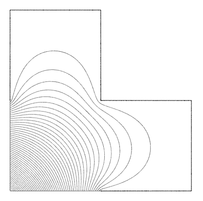
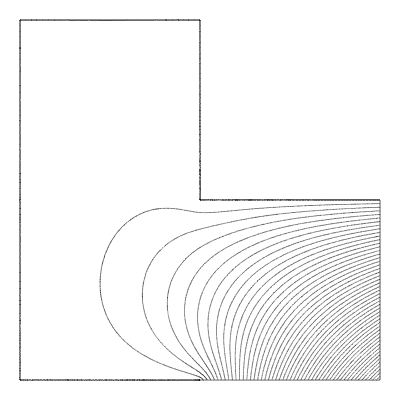
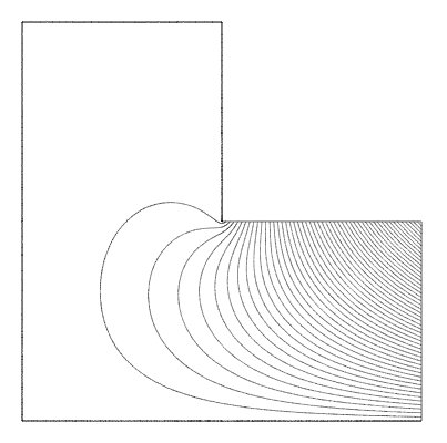
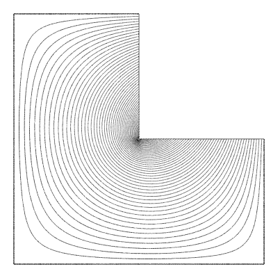
Figure 1. A “degenerate” octagon $K$, and contour plots of five of the eight basis functions for $V_{1}(K)$.

Remark 2.5 (Singular Functions in $V_{m}(K)$).

The typical singular behavior of functions in $V_{m}(K)$ near the corners of $K$ is well-understood (cf. [26, 27, 56, 57]). Since $V_{m}(K)$ is finite dimensional, any basis we choose for this space must possess such singularities in some of its components. For example, if we consider $V_{m}(K)$ for the degenerate octagon in Figure 1, and let $r=r(x)$ denote the distance from $x$ to the set of vertices, then the typical leading-singularity behavior of functions in this space is $r^{2}\ln r$ near each of the five vertices at $\pi/2$ internal angles, and $r^{2/3}$ near the vertex at the $3\pi/2$ internal angle.

Definition 2.6 (Global Poisson Space).

The global Poisson space corresponding to the partition $\mathcal{T}=\{K\}$ is

(9) $$V_{m}=V_{m}(\mathcal{T})=\{v\in C(\overline{\Omega}):\,v|_{K}\in V_{m}(K)\mbox{ for each }K\in\mathcal{T}\}~{},$$

and a unisolvent set of degrees of freedom is given by

(10) $$v(z)\;\,\forall z\in\mathcal{V}\quad,\quad\int_{e}vp\,ds\;\,\forall p\in\mathbb{P}_{m-2}(e)\;\,\forall e\in\mathcal{E}\quad,\quad\int_{K}vp\,dx\;\,\forall p\in\mathbb{P}_{m-2}(K)\;\,\forall K\in\mathcal{T}~{}.$$

As with the local Poisson spaces, we may naturally decompose $V_{m}$ into vertex, edge and interior functions,

(11) $$V_{m}=V_{m}^{\mathcal{V}}\oplus V_{m}^{\mathcal{E}}\oplus V_{m}^{\mathcal{T}}~{}.$$

We clearly have

(12) $$\dim V_{m}={\rm card}(\mathcal{T})\,\binom{m}{2}+{\rm card}(\mathcal{E})\,(m-1)+{\rm card}(\mathcal{V})~{},$$

and dimension of the space $V_{m}\cap\mathcal{H}$ is suitably reduced by replacing $\mathcal{V}$ and $\mathcal{E}$ in (12), with the non-Dirichlet vertices $\mathcal{V}^{\prime}\not\subset\partial\Omega_{D}$ and edges $\mathcal{E}^{\prime}\not\subset\partial\Omega_{D}$.

Remark 2.7.

An obvious variant of the global space described above might include a mixture standard finite elements on triangles and/or rectangles throughout much of the domain, connected to the polygonal Poisson elements by matching polynomial basis functions along shared edges. The restrictions that a computational cell $K$ is a polygon and that the boundary data is piecewise polynomial on $\partial K$ may be relaxed as well, again provided that there is a convenient mechanism enforcing agreement at interfaces between elements. As will be seen below, the Nyström approach readily provides the flexibility to explore such variants.

2.1. Integral representations of functions in $V_{m}(K)$

Remark 2.8 (Polynomial Solutions of Poisson Problems with Polynomial Sources).

Suppose that $p\in\mathbb{P}_{j}(\mathbb{R}^{n})$ is homogeneous and of degree $j$, i.e. $p(cx)=c^{j}p(x)$, and define $q\in\mathbb{P}_{j+2}(\mathbb{R}^{n})$ by

(13) $$q(x) =\sum_{k=0}^{[j/2]}\frac{(-1)^{k}\Gamma(n/2+j-k)}{\Gamma(n/2+j+1)(k+1)!}\left(\frac{|x|^{2}}{4}\right)^{k+1}\,\Delta^{k}p(x)~{},$$

where $[j/2]$ denotes the integer part of $j/2$. It is shown in [31, Theorem 2] that $\Delta q=p$. Now recall that $v\in V_{m}^{K}(K)$ satisfies $\Delta v=p$ in $K$ for some $p\in\mathbb{P}_{m-2}(K)$, with $v=0$ on $\partial K$. So we see that there is a $q\in\mathbb{P}_{m}(K)$ for which $w=v-q$ satisfies $\Delta w=0$ in $K$, with $w=-q\in\mathbb{P}_{m}(\partial K)$ on $\partial K$.

A practical consequence of Remark 2.8 is that the computation of any function in $V_{m}(K)=V^{K}_{m}(K)\oplus V^{\partial K}_{m}(K)$ is reduced to solving problems of the form

(14) $$\Delta w=0\mbox{ in }K\quad,\quad w=g\in\mathbb{P}_{m}(\partial K)\mbox{ on }\partial K~{}.$$

Let $G(x,y)$ denote the fundamental solution for the Laplacian,

(15) $$G(x,y)=\frac{1}{2\pi}\,\ln\frac{1}{|x-y|}~{}.$$

We may express the solution of (14) as a double-layer potential,

(16) $$w(x)=\int_{\partial K}\frac{\partial G(x,y)}{\partial n(y)}\,\phi(y)\,ds(y)\mbox{ for }x\in K~{},$$

where the density $\phi$ satisfies the second-kind integral equation

(17) $$\frac{\phi(x)}{2}-\int_{\partial K}\frac{\partial G(x,y)}{\partial n(y)}\,\phi(y)\,ds(y)=-g(x)\mbox{ for }x\in\partial K~{}.$$

Here and following, $n=n(y)$ denotes the outward unit normal at $y$ to the domain under consideration. The basic approach of this paper is to approximate $w\in V_{m}(K)$ via (16)-(17) by Nyström discretizations, as discussed in Section 3. In contrast, the BEM-FEM approach expresses $w$ as a combination of single- and double-layer potentials,

(18) $$w(x)=\int_{\partial K}G(x,y)\,\psi(y)\,ds(y)-\int_{\partial K}\frac{\partial G(x,y)}{\partial n(y)}\,g(y)\,ds(y)\mbox{ for }x\in K~{},$$

where the density $\psi$ satisfies the first-kind integral equation

(19) $$\int_{\partial K}G(x,y)\,\psi(y)\,ds(y)=\frac{g(x)}{2}+\int_{\partial K}\frac{\partial G(x,y)}{\partial n(y)}\,g(y)\,ds(y)\mbox{ for }x\in\partial K~{}.$$

If (17) and (19) are to be understood pointwise, then the left-hand side of (17) and the right-hand side of (19) must be modified at each corner $z\in\partial K$ (cf. [34]). For example, if the interior angle at $z$ is $\alpha\pi$, then (17) becomes

(20) $$\left(1-\frac{\alpha}{2}\right)\phi(z)-\int_{\partial K}\frac{\partial G(z,y)}{\partial n(y)}\,\phi(y)\,ds(y)=-g(z)~{}.$$

In practice, it is more convenient to use a modified form that provides a smoother integrand and does not require specific knowledge of the angle at $z$. In particular, if we take $\partial K^{\prime}$ to denote $\partial K$ without the corners, we have

(21) $$\frac{\phi(x)+\phi(z)}{2}-\int_{\partial K}\frac{\partial G(x,y)}{\partial n(y)}(\phi(y)-\phi(z))\,ds(y)=-g(x)\mbox{ for }x\in\partial K^{\prime}\cup\{z\}~{}.$$

Remark 2.9.

The derivation of (18)-(19) from Green’s formulas reveals that $\psi=\partial w/\partial n$, so the solution of (19) directly provides a Dirichlet-to-Neumann Map $g\mapsto\partial w/\partial n$. In contrast, the density $\phi$ in (17) is given by $\phi=v-g$, where $v$ is the unique solution of the complementary exterior Neumann problem

$$\Delta v=0\mbox{ in }\mathbb{R}^{2}\setminus\overline{K}\quad,\quad\frac{\partial v}{\partial n}=\frac{\partial w}{\partial n}~{},$$

and $v=o(1)$ uniformly in all directions as $|x|\to\infty$. As with the discussion of singular behavior in $V_{m}(K)$ in Remark 2.5, the singular behavior of the densities $\phi,\psi$ near corners is well-understood. Let $z\in\partial K$ be a corner with interior angle $\alpha\pi$, and let $x\in\partial K$ be near $z$. If $\alpha\in(0,2)$ is irrational, we have

1. $\psi(x)\sim|x-z|^{\alpha^{-1}-1}$ as $|x-z|\to 0$. So $\psi$ is expected to blow up near non-convex corners ($\alpha\in(1,2)$), and its tangential derivative is expected to blow up at convex corners ($\alpha\in(0,1)$).

2. $\phi(x)-\phi(z)\sim|x-z|^{\sigma^{-1}}$ as $|x-z|\to 0$, where $\sigma=\max(\alpha,2-\alpha)\geq 1$. So $\phi$ will be bounded at all corners, but its tangential derivative will typically blow up at each non-straight corner. In the case that $w$ is smooth in $K$, the complementary $v$ does not “inherit” any singular behavior from $w$ via the Neumann boundary condition, and we have $\sigma=2-\alpha$.

In the case of rational $\alpha$, logarithmic terms may appear in the asymptotic expansions of $\phi$ and $\psi$, but they are only the dominant terms in the expansion when: $\alpha=1/2$ for $\psi$, where we have $\psi(x)\sim|x-z|\,\ln|x-z|$ as $|x-z|\to 0$; or $\alpha=3/2$ and $w$ is smooth, where $\phi(x)-\phi(z)\sim|x-z|^{2}\,\ln|x-z|$ as $r\to 0$. In any case, $\phi$ is Hölder continuous.

2.2. A Hierarchical Basis for $V_{m}(K)$

The decomposition $V_{m}(K)=V_{m}^{K}(K)\oplus V_{m}^{\partial K}(K)$ makes it clear that a basis for $\mathbb{P}_{m-2}(K)$ yields a corresponding basis for $V_{m}^{K}(K)$, and a basis for $\mathbb{P}_{m}(\partial K)$ yields a corresponding basis for $V_{m}^{\partial K}(K)$. In light of Remark 2.8, it is convenient to choose a basis for $\mathbb{P}_{m-2}(K)$ in terms of translated monomials, centered at some convenient point $z\in K$,

(22) $$\mathbb{P}_{m-2}(K)=\mbox{span}\{(x-z)^{\beta}=(x_{1}-z_{1})^{\beta_{1}}(x_{2}-z_{2})^{\beta_{2}}:\;|\beta|=\beta_{1}+\beta_{2}\leq m-2\}~{}.$$

Such bases are naturally hierarchical in polynomial degree.

Given an edge $e\subset\partial K$, with endpoints $z,z^{\prime}$, we construct a hierarchical basis for $\mathbb{P}_{m}(e)$ as follows. Let $\lambda_{z}^{e},\lambda_{z^{\prime}}^{e}\in\mathbb{P}_{1}(e)$ be the corresponding barycentric coordinates for $e$, defined by $\lambda_{z}^{e}(z^{\prime})=\lambda_{z^{\prime}}^{e}(z)=\delta_{zz^{\prime}}$. For $2\leq j\leq m$, we define $b_{j}^{e}(x)=\hat{L}_{j}(\lambda_{z}^{e}(x)-\lambda_{z^{\prime}}^{e}(x))$, where $\hat{L}_{j}$ is the integrated Legendre polynomial of degree $j$ (cf. [48]). These are given in terms of the standard Legendre polynomials $L_{i}$, with normalization $L_{i}(1)=1$, by $\hat{L}_{j}(t)=\int_{-1}^{t}L_{j-1}(s)\,ds=(L_{j}(t)-L_{j-2}(t))/(2j-1)$. We see that $b_{j}^{e}(z)=b_{j}^{e}(z^{\prime})=0$, and a basis for $\mathbb{P}_{m}(e)$ that is hierarchical in polynomial degree is

(23) $$\{\lambda_{z}^{e},\lambda_{z^{\prime}}^{e}\}\cup\{b_{2}^{e},\ldots,b_{m}^{e}\}\doteq\mathcal{B}_{1}^{e}\cup\mathcal{B}_{m}^{e}~{}.$$

Given a vertex $z\in\mathcal{V}(K)$, the function $\lambda_{z}\in\mathbb{P}_{1}(\partial K)$ is determined by the conditions $\lambda_{z}(z^{\prime})=\delta_{zz^{\prime}}$ for all $z^{\prime}\in\mathcal{V}(K)$; so $\lambda_{z}|_{e}=\lambda_{z}^{e}$ if $z$ is an endpoint of $e$. Clearly $\mathcal{B}_{1}=\{\lambda_{z}:\;z\in\mathcal{V}(K)\}$ is a basis for $\mathbb{P}_{1}(\partial K)$. Each element $b_{j}^{e}$ of $\mathcal{B}_{m}^{e}$ vanishes at the endpoints of $e$, so we continuously extend it by $0$ to $\partial K$. Finally, a hierarchical basis for $\mathbb{P}_{m}(\partial K)$, is given by

(24) $$\mathcal{B}_{1}\cup\left(\bigcup_{e\in\mathcal{E}(K)}\mathcal{B}_{m}^{e}\right)\doteq\mathcal{B}_{1}\cup\mathcal{B}_{m}~{}.$$

3. Nyström Approximation Second-Kind Integral Equations

As was seen in the previous section, the computation of $v\in V_{m}(K)$ is reduced to the computation of a harmonic function $w$ on $K$ with prescribed Dirichlet data, and we opt to do so via second-kind integral equations. Nyström methods [42, 43] for second-kind integral equations, in their most basic forms, are derived by replacing the boundary integral with a suitable quadrature, and sampling the resulting equation at the quadrature points. The performance of the method is directly tied to the performance of the underlying quadrature, and we will briefly describe the version proposed by Kress [33] for problems of the sort that we here consider, after first looking more closely at the components of the integrand.

Recalling (21), for $x\in\partial K$ near or at a vertex/corner $z$, we have

(25) $$\frac{\phi(x)+\phi(z)}{2}+\int_{\partial K}F(x,y)(\phi(y)-\phi(z))\,ds(y)=-g(x)\;,\;F(x,y)=-\frac{\partial G(x,y)}{\partial n(y)}=-\frac{(x-y)\cdot n(y)}{2\pi\,|x-y|^{2}}~{}.$$

We note that $F(x,y)=0$ when $x$ and $y$ are on the same (straight) edge of $\partial K$. More generally, for any fixed $x\in\partial K$, $F(x,y)$ is a piecewise smooth function of $y\in\partial K$, with bounded jump-discontinuities at the corners of $\partial K$. In fact, for any $x\in\partial K$, $F(x,y)$ is analytic in the interior of each edge. This is not to say that $F(x,y)$ exhibits no difficult behavior: if $x\in\partial K$ is very near (but not at) a corner $z$, then $F(x,y)$ and its tangential derivatives in $y$ are very large as $y$ approaches $z$ along the edge not containing $x$. More specifically, if $x$ and $y$ are on opposite straight edges sharing $z$, and the interior angle at $z$ is $\alpha\pi$ then

$$\lim_{y\to z}F(x,y)=\frac{\sin(\alpha\pi)}{2\pi|x-z|}~{},$$

where $y$ is understood to approach $z$ along the edge they share. For $x\in\partial K$ we choose $z=z(x)$ to be the nearest vertex in terms of distance along the boundary, breaking ties arbitrarily if $x$ is at the midpoint of an edge. The fact that the integrand in (25) vanishes at $y=z$ makes it easier to approximate the integral by simple quadrature.

The basic quadrature employed by Kress [33] for $f\in C[0,1]$ is obtained by applying the uniform trapezoid rule after a sigmoidal change-of-variable,

$$\int_{0}^{1}f(t)\,dt=\int_{0}^{1}f(\eta(\tau))\eta^{\prime}(\tau)\,d\tau\approx\frac{1}{n}\sideset{}{{}^{\prime\prime}}{\sum}_{k=0}^{n}f(\eta(k/n))\eta^{\prime}(k/n)=\frac{1}{n}\sum_{k=1}^{n-1}f(\eta(k/n))\eta^{\prime}(k/n)~{},$$

where the transformation $t=\eta(\tau)$ is given by

$$\eta(\tau)=\frac{[c(\tau)]^{p}}{[c(\tau)]^{p}+[1-c(\tau)]^{p}}\quad,\quad c(\tau)=\left(\frac{1}{2}-\frac{1}{p}\right)(2\tau-1)^{3}+\frac{1}{p}(2\tau-1)+\frac{1}{2}~{},$$

and $p\geq 2$ is an integer. It is straight-forward to see that $\eta$ has a root of order $p$ at $0$, and $1-\eta$ has a root of order $p$ at $1$. A careful convergence analysis of this quadrature is given in [33], showing that it is convergent on $C[0,1]$, and, for the kinds of integrands we encounter here, of increasingly higher-order in $n$ as $p$ is increased. If $e$ is a smooth (curved) edge, with smooth parametrization $x_{e}=x_{e}(t)$ satisfying $|x_{e}^{\prime}(t)|\geq\sigma>0$, we have the quadrature

(26) $$\int_{e}f\,ds=\int_{0}^{1}f(x(t))|x_{e}^{\prime}(t)|\,dt\approx\sideset{}{{}^{\prime\prime}}{\sum}_{k=0}^{n}f(x_{k}^{e})\omega_{k}=\sum_{k=1}^{n-1}f(x_{k}^{e})\omega_{k}~{},$$

where $\omega_{k}=\eta^{\prime}(k/n)\,|x_{e}^{\prime}(\eta(k/n))|/n$ and $x_{k}^{e}=x_{e}(\eta(k/n))$. In the case of a straight edge $e$ having endpoints $z,z^{\prime}$, these weights and points simplify to

(27) $$\omega_{k}=\eta^{\prime}(k/n)\,|e|/n\quad,\quad x_{k}^{e}=(1-\eta(k/n))z+\eta(k/n)z^{\prime}=\eta(1-k/n)z+\eta(k/n)z^{\prime}~{}.$$

Keeping a fixed $n$ and $p$ for all edges, we take a global enumeration of the quadrature points and weights (including vertices), $\{(x_{j},\omega_{j}):\,1\leq j\leq M=nN\}$. The Nyström linear system corresponding to (25) is given by

(28) $$\frac{\phi_{i}+\phi_{k}}{2}+\sum_{j=1}^{M}F(x_{i},x_{j})(\phi_{j}-\phi_{k})\omega_{j}=-g(x_{i})~{},$$

where $x_{k}=z(x_{i})$ is the vertex nearest $x_{i}$. The approximation $\tilde{w}(x)\approx w(x)$ for $x\in K$ is given by

(29) $$\tilde{w}(x)=-\sum_{j=1}^{M}F(x,x_{j})\phi_{j}\omega_{j}~{}.$$

We demonstrate the efficacy of the Nyström scheme in obtaining accurate approximations to solutions of a couple of example boundary value problems (14) that present challenges similar to those that arise in the construction of $V_{m}(K)$. In particular, these examples deal with regions that have multiple corners, so the corresponding densities $\phi$ exhibit singularities as described in Remark 2.9. In both cases a harmonic function $w$ is given, and the (non-polynomial) Dirichlet data is taken from $w$. Relative and/or absolute errors in the Nyström approximation of $w$ are given at several points in the interior of $K$ for these examples, when $n$ points are used on each edge and the parameter $p=6$ is used for the quadrature.

Example 3.1.

Let $K$ be the L-shaped hexagon with vertices at $(0,0),(1,0),(1,1),(-1,1),(-1,-1),(0,-1)$, and take $w=\ln|x-\hat{x}|$, where $\hat{x}=(10,0)$. Although $w$ is smooth in $K$, the corresponding density $\phi$ will have singular behavior as discussed before. More specifically, $\psi\sim|x-z|^{2/3}$ near each of the five corners $z$ having interior angle $\pi/2$, and $\psi\sim|x|^{2}\ln|x|$ near the corner at the origin having interior angle $3\pi/2$. In Table 1, relative errors in the Nyström approximation of $w$ are given at four points in $K$, and clearly demonstrate the high-order convergence as the number of points per edge increases, as well as the accuracy even when few points are used.

Table 1. Relative errors at five points for the Nyström approximation of $w=\ln|x-\hat{x}|$ in an L-shaped hexagon.

$n$	(0.5,0.5)	(0.1,0.1)	(0.01,0.01)	(0.001,0.001)	(0.999,0.001)
16	5.954e-07	1.168e-05	3.231e-06	3.142e-07	1.912e-05
32	1.077e-10	1.976e-07	2.530e-08	3.379e-07	1.298e-06
64	6.565e-13	1.628e-09	5.423e-10	3.584e-09	1.867e-08
128	9.857e-15	4.329e-11	2.062e-11	1.343e-11	2.897e-10
256	1.971e-16	4.990e-13	9.927e-13	1.341e-12	1.309e-11
512	0.000e+00	3.680e-15	7.120e-14	7.175e-14	6.532e-13
1024	0.000e+00	5.811e-16	4.631e-15	7.522e-15	3.941e-14
2048	0.000e+00	0.000e+00	1.929e-16	1.929e-16	5.457e-15

Example 3.2.

Here we take $K=K(\alpha)=\{x=(r\cos\theta,r\sin\theta)\,:\;\ 0<r<1,0<\theta<\alpha\pi\}$ to be the sector of the unit circle with interior opening angle $\alpha\pi$, and $w=r^{1/\alpha}\sin(\theta/\alpha)$. This example provides a situation like many we expect to encounter in practice, where both $\phi$ and $w$ have singular behavior near a corner. The interior angles at the other two corners, $(0,1)$ and $(\cos\alpha\pi,\sin\alpha\pi)$, are both $\pi/2$. We consider the case $K(3/2)$, a “circular L-shape”. We have $\phi(x)\sim|x-z|^{2/3}$ near each of the three corners $z$. Since $w=0$ at the origin, we provide both relative and absolute approximation errors at a few points near the origin. The results for $K(3/2)$ are given in Table 2. We again see similar high-order convergence.

Table 2. Relative and absolute errors at three points for the Nyström approximation of $w=r^{2/3}\sin(2\theta/3)$ on the circular L-shape $K(3/2)$.

	(0.1,0.1)		(0.01,0.01)		(0.001,0.001)
$n$	Rel	Abs	Rel	Abs	Rel	Abs
16	9.518e-03	1.292e-03	3.065e-02	8.963e-04	5.558e-02	3.501e-04
32	2.841e-05	3.856e-06	1.237e-02	3.616e-04	8.311e-02	5.236e-04
64	2.763e-08	3.750e-09	2.910e-05	8.510e-07	3.303e-05	2.228e-07
128	9.083e-11	1.233e-11	1.715e-09	5.016e-11	2.008e-06	1.265e-08
256	2.708e-13	3.675e-14	7.337e-12	2.145e-13	1.590e-10	1.002e-12
512	8.180e-16	1.110e-16	4.675e-14	1.367e-15	8.468e-13	5.334e-15
1024	3.190e-14	4.330e-15	2.442e-13	7.140e-15	9.173e-13	5.778e-15
2048	2.699e-14	3.664e-15	2.442e-13	7.140e-15	1.339e-12	8.432e-15

4. Interpolation in $V_{m}$

We consider some properties of the interpolation operator $\mathfrak{I}_{m}:C(\overline{\Omega})\to V_{m}$ defined by

(30) $$\begin{cases}\left(\mathfrak{I}_{m}v\right)(z)=v(z)&\;\,\forall z\in\mathcal{V}\\ \int_{e}\left(\mathfrak{I}_{m}v\right)p\,ds=\int_{e}vp\,ds&\;\,\forall p\in\mathbb{P}_{m-2}(e)\;\,\forall e\in\mathcal{E}\\ \int_{K}\left(\mathfrak{I}_{m}v\right)p\,dx=\int_{K}vp\,dx&\;\,\forall p\in\mathbb{P}_{m-2}(K)\;\,\forall K\in\mathcal{T}\end{cases}~{},$$

both theoretically and empirically. The interpolation operator $\mathfrak{I}_{m}$ may be decomposed in such a way as to correspond to the space decomposition $V_{m}=V_{m}^{\mathcal{V}}\oplus V_{m}^{\mathcal{E}}\oplus V_{m}^{\mathcal{T}}$, namely $\mathfrak{I}_{m}=\mathfrak{I}_{m}^{\mathcal{V}}+\mathfrak{I}_{m}^{\mathcal{E}}+\mathfrak{I}_{m}^{\mathcal{T}}$, where $\mathfrak{I}_{m}^{\mathcal{V}}:C(\overline{\Omega})\to V_{m}^{\mathcal{V}}$, $\mathfrak{I}_{m}^{\mathcal{E}}:C(\overline{\Omega})\to V_{m}^{\mathcal{E}}$ and $\mathfrak{I}_{m}^{\mathcal{T}}:C(\overline{\Omega})\to V_{m}^{\mathcal{T}}$ are uniquely determined by

(31) $$\begin{cases}\left(\mathfrak{I}_{m}^{\mathcal{V}}v\right)(z)=v(z)&\;\,\forall z\in\mathcal{V}\\ \int_{e}\left(\mathfrak{I}_{m}^{\mathcal{E}}v\right)p\,ds=\int_{e}(v-\mathfrak{I}_{m}^{\mathcal{V}}v)p\,ds&\;\,\forall p\in\mathbb{P}_{m-2}(e)\;\,\forall e\in\mathcal{E}\\ \int_{K}\left(\mathfrak{I}_{m}^{\mathcal{T}}v\right)p\,dx=\int_{K}\left(v-\mathfrak{I}_{m}^{\mathcal{V}}v-\mathfrak{I}_{m}^{\mathcal{E}}v\right)p\,dx&\;\,\forall p\in\mathbb{P}_{m-2}(K)\;\,\forall K\in\mathcal{T}\end{cases}~{}.$$

We have the obvious restrictions of these interpolation operators to a single element, and we use the same symbols to denote them. On a single element $K$, it is also convenient to use $\mathfrak{I}_{m}^{\partial K}:C(\overline{K})\to V_{m}^{\partial K}(K)$ to denote the interpolation operator defined by

(32) $$\begin{cases}\left(\mathfrak{I}_{m}^{\partial K}v\right)(z)=v(z)&\;\,\forall z\in\mathcal{V}(K)\\ \int_{e}\left(\mathfrak{I}_{m}^{\partial K}v\right)p\,ds=\int_{e}(v-\mathfrak{I}_{m}^{\mathcal{V}}v)p\,ds&\;\,\forall p\in\mathbb{P}_{m-2}(e)\;\,\forall e\in\mathcal{E}(K)\end{cases}~{}.$$

So $\mathfrak{I}_{m}=\mathfrak{I}_{m}^{K}+\mathfrak{I}_{m}^{\partial K}$ on $C(\overline{K})$.

Given $v\in C(\overline{K})$, with $v=g$ on $\partial K$, we define $\tilde{g}\in C(\partial\Omega)$ by

(33) $$\tilde{g}(z)=g(z)\;\forall z\in\mathcal{V}(K)\quad,\quad\int_{e}\tilde{g}p\,ds=\int_{e}gp\,ds\;\forall p\in\mathbb{P}_{m-2}(e)\;\forall e\in\mathcal{E}(K)~{}.$$

By definition, $\mathfrak{I}_{m}^{\partial K}v$ is the solution of

(34) $$\Delta(\mathfrak{I}_{m}^{\partial K}v)=0\mbox{ in }K\quad,\quad\mathfrak{I}_{m}^{\partial K}v=\tilde{g}\mbox{ on }\partial K~{}.$$

Assuming that $g$ is continuously differentiable along each edge of $K$, we see that, for any $q\in\mathbb{P}_{m}(e)$,

$$\int_{e}\frac{\partial(g-\tilde{g})}{\partial t}\frac{\partial q}{\partial t}\,ds=\left.(g-\tilde{g})\frac{\partial q}{\partial t}\right|_{z^{\prime}}^{z}-\int_{e}(g-\tilde{g})\frac{\partial^{2}q}{\partial t^{2}}\,ds=0~{},$$

where $z,z^{\prime}$ are the endpoints of $e$, and the partial derivatives are in the tangential direction. From this orthogonality relation, it is clear that

$$|g-\tilde{g}|_{H^{1}(e)}=\inf_{p\in\mathbb{P}_{m}(e)}|g-p|_{H^{1}(e)}\;\forall e\in\mathcal{E}(K)~{}.$$

Recalling our hierarchical basis (23) for $\mathbb{P}_{m}(e)$, we have

(35) $$\tilde{g}(x) =g(z)\lambda_{z}^{e}(x)+g(z^{\prime})\lambda_{z^{\prime}}^{e}(x)+\sum_{j=2}^{m}c_{j}b_{j}^{e}(x)\quad,\quad c_{j}=\frac{(2j-1)}{2}\int_{e}\frac{\partial g}{\partial t}\,L_{j-1}(\lambda_{z}-\lambda_{z^{\prime}})\,ds~{},$$

on $e$. This follows from the relations

$$\frac{\partial b_{j}^{e}}{\partial t}=\frac{2}{|e|}\,L_{j-1}(\lambda_{z}-\lambda_{z^{\prime}})\quad,\quad\int_{e}\frac{\partial b_{j}^{e}}{\partial t}\frac{\partial b_{i}^{e}}{\partial t}\,ds=\frac{4\delta_{ij}}{(2j-1)|e|}~{}.$$

Having computed $\mathfrak{I}_{m}^{\partial K}u$ from (34), with $\tilde{g}$ given by (35), we obtain $\mathfrak{I}_{m}v=\mathfrak{I}_{m}^{K}v+\mathfrak{I}_{m}^{\partial K}v$ on $K$ via

(36) $$\int_{K}\left(\mathfrak{I}_{m}^{K}v\right)p\,dx=\int_{K}\left(v-\mathfrak{I}_{m}^{\partial K}v\right)p\,dx \;\,\forall p\in\mathbb{P}_{m-2}(K)~{}.$$

Finally, taking a translated monomial basis $\{p_{\beta}\in\mathbb{P}_{m-2}:\,|\beta|\leq m-2\}$ of $\mathbb{P}_{m-2}$, as in (22), and letting $\{\varphi_{\beta}\in H^{1}_{0}(\Omega):\,\Delta\varphi_{\beta}=p_{\beta}\;,\;|\beta|\leq m-2\}$ be the associated basis of $V_{m}^{K}(K)$, we see that the coefficients $c_{\beta}$ of $\mathfrak{I}_{m}^{K}v=\sum_{|\beta|\leq 2}c_{\beta}\varphi_{\beta}$ satisfy the negative definite linear system

(37) $$\sum_{|\beta|\leq m-2}c_{\beta}\int_{K}\varphi_{\beta}p_{\beta^{\prime}}\,dx=\int_{K}\left(v-\mathfrak{I}_{m}^{\partial K}v\right)p_{\beta^{\prime}}\,dx\;,\;\forall|\beta^{\prime}|\leq m-2~{}.$$

Using (8), this system matrix is seen to be negative definite by

$$\int_{K}\varphi_{\beta}p_{\beta^{\prime}}\,dx=-\int_{K}\nabla\varphi_{\beta}\cdot\nabla\varphi_{\beta^{\prime}}\,dx~{}.$$

Remark 4.1.

When $m=1$, $\mathfrak{I}_{m}v=\mathfrak{I}_{m}^{\partial K}v$, so interpolation in this case reduces to solving harmonic problems with interpolated boundary data (35). If $v$ is harmonic in $K$, then it can be well-approximated by functions in $V_{m}^{\partial K}(K)$, because this space contains the harmonic polynomials of degree $\leq m$, and these approximate general harmonic functions essentially as well as the entire space $\mathbb{P}_{m}(K)$ does (cf. [38, 37]).

Remark 4.2.

Although (35) provides a exact expression for the coefficients $c_{j}$ of $\tilde{g}$ on $e$ as an integral involving its tangential derivative, we found it more convenient for our interpolation experiments below to compute these coefficients in a different way. They were computed as the solution of a simple linear system derived by plugging the expression for $\tilde{g}$ from (35) into the integral identities in (33), with $p$ being the Lagrange polynomials of degree $\leq m-2$ associated with the edge. The orthogonality relations for Lagrange polynomials leads to an $(m-1)\times(m-1)$ system matrix whose only non-zero elements are on the main diagonal and second lower-diagonal, and the righthand side is adequately addressed by quadrature.

Example 4.3.

To demonstrate the interpolation properties, we consider a numerical experiment and interpolate the function $v(x)=\sin(2\pi x_{1})\sin(2\pi x_{2})$ over $\Omega=(0,1)^{2}$ on a sequence of uniformly refined meshes, see Figure 2. The expansion coefficients are determined as described above. The volume integrals in (37) are realized by means of numerical quadrature. For this purpose, we split the element $K$ into triangles by connecting the vertices $\mathcal{V}(K)$ with the center of mass. Afterwards, a $7$-point Gaussian rule is applied on each triangle and the discrete functions in $V_{m}(K)$ are treated by means of Nyström approximations, see Section 3. The relative interpolation error is plotted in Figure 3 for the $L_{2}$- as well as the $H^{1}$-norm with respect to the maximal mesh size $h_{\mathrm{max}}=\max\{h_{K}:K\in\mathcal{T}\}$. An optimal order of convergence is achieved.

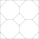
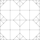
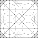
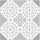
Figure 2. Initial mesh for Example 4.3 (left), and uniform refinements after $2,4$ and $6$ steps.

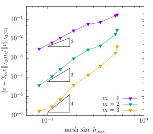
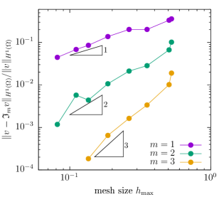
Figure 3. Relative interpolation error in $L_{2}$- and $H^{1}$-norm for Example 4.3, with $m=1,2,3$.

Example 4.4.

In a second example, we interpolate the function $v(x)=r^{2/3}\sin(2(\theta-\pi/2)/3)$ on the L-shaped domain $\Omega=(-1,1)^{2}\setminus[0,1]^{2}$. This function exhibits the typical singularity at the reentrant corner. For $m=1$, we compare the $L^{2}$-interpolation error for two families of meshes (see Figure 4). The $n^{th}$ mesh, $\mathcal{T}_{n}$, of the first family consists of one L-shaped element, $(-1/3,1/3)^{2}\setminus[0,1/3]^{2}$, and $24n^{2}$ squares of size $(3n)^{-1}\times(3n)^{-1}$; $\mathcal{T}_{n}$ has $(2n+1)(12n+1)+1$ vertices. The $n^{th}$ mesh, $\widehat{\mathcal{T}}_{n}$, of the second family consists of congruent squares such that its number of vertices, which is of the form $(k+1)(3k+1)$, is as close as possible to $(2n+1)(12n+1)+1$. The dimensions of $V_{1}(\mathcal{T}_{n})$ and $V_{1}(\hat{\mathcal{T}}_{n})$ are clearly the number of vertices in the corresponding meshes. For all square elements in either mesh, the local spaces are the bilinear functions. If $K$ is the $L$-shaped element in $\mathcal{T}_{n}$, then $\dim V_{1}(K)=6n+2$, and $V_{1}(K)$ contains functions having the correct singular behavior at the reentrant corner.

We study the convergence of the relative interpolation error in $L_{2}(\Omega)$ with respect to the number of degrees of freedom (DoF) for both families of meshes. The optimal convergence behavior for the second family of meshes for an arbitrary smooth function is $\mathcal{O}(\mathrm{DoF}^{-1})$, but we neither expect or obtain that behavior for the given $v$, because of its singularity at the origin. In Table 3, the relative interpolation error in the $L_{2}$-norm is given for the two sequences of meshes with comparable numbers of degrees of freedom. Furthermore, the numerical order of convergence (noc) is given. This is an estimate of the exponent $q$ in the error model $C\mathrm{DoF}^{-q}$. Since the function $v$ has a singularity, the convergence slows down for the standard bilinear elements on the uniform sequence of quadrilateral meshes. But, the optimal order of convergence is recovered for the uniform sequence with a fixed L-shaped element, because the local space associated with that element contains naturally functions with the correct singular behavior near the corner.

Figure 4. First four meshes of first family (top), and second family, for Example 4.4. The fourth mesh in the first family has edge-length $1/12$ for each of its squares, and the fourth mesh in the second family has edge-length $1/11$ for each of its squares.

Table 3. Relative $L_{2}$-error (err) and numerical order of convergence (noc) with respect to the number of degrees of freedom (DoF) for first order interpolation ($m=1$) of $v=r^{2/3}\sin(2(\theta-\pi/2)/3)$ in Example 4.4.

First Family			Second Family
DoF	err	noc	DoF	err	noc
$40$	3.238e-03	–	$40$	1.263e-02	–
$126$	8.015e-04	1.22	$133$	4.003e-03	0.96
$260$	3.549e-04	1.12	$280$	2.042e-03	0.90
$442$	1.989e-04	1.09	$408$	1.463e-03	0.89
$672$	1.269e-04	1.07	$833$	7.848e-04	0.87
$950$	8.789e-05	1.06	$1045$	6.452e-04	0.86
$1276$	6.439e-05	1.05	$1281$	5.415e-04	0.86

5. Dirichlet Boundary Conditions, Curvilinear Elements

As suggested in Remark 2.7 and illustrated in Example 3.2, the Nyström approach for evaluating functions that solve local Poisson problems readily accommodates curvilinear elements and non-polynomial data. As such, curved boundaries or interior interfaces may be addressed more directly, without resorting to polygonal approximations of these curves or mappings from polygonal reference elements (e.g. isoparametric elements, cf. [47, 35, 9]). Although the treatment of curved boundary and interior edges in our framework will be investigated more thoroughly in later work, we here provide some indication of how our approach may be used to address Dirichlet boundary conditions on straight or curved edges, after first making a few general remarks about necessary changes to the description of $V_{m}(K)$ that must be made to accommodate curved edges.

We first remark that, if $K$ is a not a (straight-edged) polygon, the definition of $V_{m}(K)$ must be either adjusted or properly interpreted. More specifically, if $e$ is a curved edge of $K$, the defintion of $\mathbb{P}_{m}(e)$, i.e. the polynomials of degree at most $m$ on $e$, needs clarification. One fairly natural approach is to define $\mathbb{P}_{m}(e)$ as the space of polynomials of degree at most $m$ with respect to arc length on $e$. We will call this approach the Type 1 version of $\mathbb{P}_{m}(e)$. In this case, $\dim\mathbb{P}_{m}(e)=m+1$. A potential drawback of this approach is that it does not generally lead to the inclusion $\mathbb{P}_{m}(K)\subset V_{m}(K)$, so we are not guaranteed the approximation quality of $\mathbb{P}_{m}(K)$. A second approach to defining $\mathbb{P}_{m}(e)$ for a curved edge $e$ is to take it to be the trace on $e$ of $\mathbb{P}_{m}(\mathbb{R}^{2})$. We will call this approach the Type 2 version of $\mathbb{P}_{m}(e)$. For the Type 2 version, we typically have $\dim\mathbb{P}_{m}(e)=(m+2)(m+1)/2$, which leads to a larger space $V_{m}(K)$, but yields the desired inclusion $\mathbb{P}_{m}(K)\subset V_{m}(K)$. When $e$ is a straight edge, the Type 1 and Type 2 versions of $\mathbb{P}_{m}(e)$ yield the same space. Note that one must revise the definition of the degrees of freedom associated with a curved edge in the Type 2 case. Basic differences between the two approaches to defining $\mathbb{P}_{m}(e)$ are illustrated in Example 5.1. A thorough investigation of these two approaches, and of the practical and theoretical treatment of curved edges more generally, is a topic of subsequent work.

Example 5.1.

Let $K=K_{h}=\{x=(r\cos\theta,r\sin\theta):\;0<r<h\,,\,0<\theta<\alpha\pi\}$ for some fixed $0<\alpha<2$, with two straight edges and one curved edge $e=\{x=(h\cos\theta,h\sin\theta):\;0\leq\theta\leq\alpha\pi\}$. We compare the two approaches to defining $\mathbb{P}_{m}(e)$ in the case $m=1$. For the Type 1 space, we have $P_{1}(e)=\mathrm{span}\{1,\theta\}$. For the Type 2 space, we have $\mathbb{P}_{1}(e)=\mathrm{span}\{1,\cos\theta,\sin\theta\}$. Natural bases for these two approaches are plotted in Figure 5, with respect to $\theta$, for the choices $\alpha=1/2$ and $\alpha=3/2$. The Type 1 basis functions are what one would expect, and undergo no qualitative changes as $\alpha$ varies. The Type 2 basis functions were chosen with respect to the endpoints and midpoint of the edge, such that each basis function has the value one at one of these three points, and the value zero at the two others. The qualitative behavior of Type 2 basis functions clearly depends on $\alpha$ here.

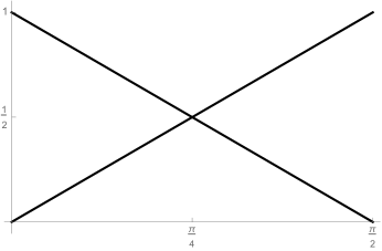
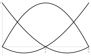
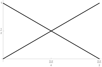
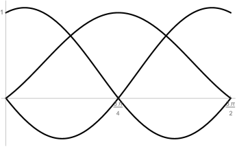
Figure 5. Bases of the two types of spaces $\mathbb{P}_{1}(e)$ for the circular arc in Example 5.1. First column corresponds to Type 1, and second column to Type 2. First row corresponds to $\alpha=1/2$, and second row to $\alpha=3/2$.

We now turn to the treatment of Dirichlet boundary conditions. Let $K$ be curvilinear polygon such that $\partial K_{D}\doteq\partial K\cap\partial\Omega\neq\emptyset$, and suppose we wish to prescribe boundary values $g$ that are continuous and piecewise smooth on $\partial K_{D}$. At this stage, we assume that any curved edges are contained in $\partial K_{D}$; so all interior edges are straight. We take $g_{D}\in C(\partial K)$ to be $g$ on $\partial K_{D}$, $0$ on edges not adjacent to $\partial K_{D}$, and linear on edges adjacent to $\partial K_{D}$. We employ the following local linear (and affine) spaces:

(38) $$V_{m}^{K}(K) =\{v\in H^{1}_{0}(K):\;\Delta v\in\mathbb{P}_{m-2}(K)\mbox{ in }K\}~{},$$

(39) $$V_{m}^{\partial K,0}(K) =\{v\in H^{1}(K):\;\Delta v=0\mbox{ in }K\;,\,v\in\mathbb{P}_{m}^{0,D}(\partial K)\mbox{ on }\partial K\}~{},$$

(40) $$V_{m}^{\partial K,g}(K) =v_{g}+V_{m}^{\partial K,0}(K)~{},$$

where $\mathbb{P}_{m}^{0,D}(\partial K)$ are those functions in $C(\partial K)$ whose restriction to any edge $e\not\subset\partial K_{D}$ is $\mathbb{P}_{m}(e)$, and whose restriction to to any edge $e\subset\partial K_{D}$ is $0$. The function $v_{g}$ satisfies

$$\Delta v_{g}=0\mbox{ in }K\quad,\quad v=g_{D}\mbox{ on }\partial K~{}.$$

The local affine space used in the global approximation is $V_{m,g,D}(K)=V_{m}^{K}(K)+V_{m}^{\partial K,g}(K)$.

Example 5.2.

We consider a single element

$$K=K_{h}=\{(x_{1},x_{2})\in\mathbb{R}^{2}:\;0\leq x_{1}\leq h\,,\,\sin(2\pi x_{1}/h)/4\leq x_{2}\leq h\}~{},$$

(see Figure 6). We consider the convergence of the interpolation error $v-\mathfrak{I}_{1}v$ in $L^{2}(K)$ with respect to $h$ for $\mathfrak{I}_{1}v\in V_{1,g,D}(K)$ and two different smooth functions $v$. Since $m=1$, $\mathfrak{I}_{1}v$ that agrees with $v$ on the curved edge, is equal to the linear interpolant of $v$ on each of the three straight edges. So computing $\mathfrak{I}_{1}v$ requires the solution of a single integral equation.

If we had the inclusion $\mathbb{P}_{1}(K)\subset V_{1,g,D}(K)$, standard interpolation error estimates (cf. [20, Theorem 1.103]) would yield

$$\|v-\mathfrak{I}_{1}v\|_{L^{2}(K)}\leq ch^{2}|v|_{H^{2}(K)}$$

for $v\in H^{2}(K)$. Though we are not guaranteed, and will typically not have, the inclusion $\mathbb{P}_{1}(K)\subset V_{1,g,D}(K)$, we still desire such quadratic convergence with respect to $h$ in practice. The experiments presented in Table 4 demonstrate this quadratic convergence in $h$ for two smooth functions by considering ratios of successive errors as $h$ is halved.

Figure 6. Element $K_{h}$ from Example 5.2.

Table 4. $L^{2}$ interpolation error, $\mathrm{error}=\|v-\mathfrak{I}_{1}v\|_{L^{2}(K)}/|v|_{H^{2}(K)}$, for $K=K_{h}$ from Example 5.2.

	$v=x^{3}-3xy^{2}+5(x^{2}-y^{2})$		$v=e^{x}+e^{y}$
$h$	error	ratio	error	ratio
$2^{-3}$	5.4199e-04		1.5157e-03
$2^{-4}$	1.3546e-04	4.0011	3.7899e-04	3.9994
$2^{-5}$	3.3856e-05	4.0010	9.4737e-05	4.0004
$2^{-6}$	8.4628e-06	4.0006	2.3682e-05	4.0004
$2^{-7}$	2.1155e-06	4.0003	5.9201e-06	4.0002
$2^{-8}$	5.2886e-07	4.0002	1.4800e-06	4.0001

6. Acknowledgements

The work of JO on this paper was supported by the National Science Foundation under Grant No. DMS-1414365. AA thanks the NPDE-TCA for supporting JO’s visit to IIT Kanpur that laid the foundation for this paper.

References

- [1] B. Ahmad, A. Alsaedi, F. Brezzi, L. D. Marini, and A. Russo. Equivalent projectors for virtual element methods. Comput. Math. Appl., 66(3):376–391, 2013.
- [2] P. Antonietti, M. Bruggi, S. Scacchi, and M. Verani. On the virtual element method for topology optimization on polygonal meshes: A numerical study. Comput. Math. Appl., 2017.
- [3] P. F. Antonietti, L. Beirão da Veiga, D. Mora, and M. Verani. A stream virtual element formulation of the Stokes problem on polygonal meshes. SIAM J. Numer. Anal., 52(1):386–404, 2014.
- [4] L. Beirão da Veiga, A. Chernov, L. Mascotto, and A. Russo. Basic principles of virtual elements on quasiuniform meshes. Math. Models Methods Appl. Sci., 26(8):1567–1598, 2016.
- [5] L. Beirão da Veiga, F. Brezzi, A. Cangiani, G. Manzini, L. D. Marini, and A. Russo. Basic principles of virtual element methods. Math. Models Methods Appl. Sci., 23(1):199–214, 2013.
- [6] L. Beirão da Veiga, F. Brezzi, L. D. Marini, and A. Russo. The hitchhiker’s guide to the virtual element method. Math. Models Methods Appl. Sci., 24(8):1541–1573, 2014.
- [7] L. Beirão da Veiga and G. Manzini. A virtual element method with arbitrary regularity. IMA J. Numer. Anal., 34(2):759–781, 2014.
- [8] M. F. Benedetto, S. Berrone, A. Borio, S. Pieraccini, and S. Scialò. Order preserving SUPG stabilization for the virtual element formulation of advection-diffusion problems. Comput. Methods Appl. Mech. Engrg., 311:18–40, 2016.
- [9] C. Bernardi. Optimal finite-element interpolation on curved domains. SIAM J. Numer. Anal., 26(5):1212–1240, 1989.
- [10] J. Bonelle, D. A. Di Pietro, and A. Ern. Low-order reconstruction operators on polyhedral meshes: application to compatible discrete operator schemes. Comput. Aided Geom. Design, 35/36:27–41, 2015.
- [11] J. Bonelle and A. Ern. Analysis of compatible discrete operator schemes for elliptic problems on polyhedral meshes. ESAIM Math. Model. Numer. Anal., 48(2):553–581, 2014.
- [12] J. Bonelle and A. Ern. Analysis of compatible discrete operator schemes for the Stokes equations on polyhedral meshes. IMA J. Numer. Anal., 35(4):1672–1697, 2015.
- [13] F. Brezzi and L. D. Marini. Virtual element and discontinuous Galerkin methods. In Recent developments in discontinuous Galerkin finite element methods for partial differential equations, volume 157 of IMA Vol. Math. Appl., pages 209–221. Springer, Cham, 2014.
- [14] A. Cangiani, Z. Dong, E. H. Georgoulis, and P. Houston. -version discontinuous Galerkin methods for advection-diffusion-reaction problems on polytopic meshes. ESAIM Math. Model. Numer. Anal., 50(3):699–725, 2016.
- [15] J. Collis and P. Houston. Adaptive discontinuous Galerkin methods on polytopic meshes. In Advances in discretization methods, volume 12 of SEMA SIMAI Springer Ser., pages 187–206. Springer, [Cham], 2016.
- [16] D. Copeland, U. Langer, and D. Pusch. From the boundary element domain decomposition methods to local Trefftz finite element methods on polyhedral meshes. In Domain decomposition methods in science and engineering XVIII, volume 70 of Lect. Notes Comput. Sci. Eng., pages 315–322. Springer, Berlin, 2009.
- [17] D. A. Di Pietro and A. Ern. A hybrid high-order locking-free method for linear elasticity on general meshes. Comput. Methods Appl. Mech. Engrg., 283:1–21, 2015.
- [18] D. A. Di Pietro and A. Ern. Hybrid high-order methods for variable-diffusion problems on general meshes. C. R. Math. Acad. Sci. Paris, 353(1):31–34, 2015.
- [19] D. A. Di Pietro, A. Ern, and S. Lemaire. An arbitrary-order and compact-stencil discretization of diffusion on general meshes based on local reconstruction operators. Comput. Methods Appl. Math., 14(4):461–472, 2014.
- [20] A. Ern and J.-L. Guermond. Theory and practice of finite elements, volume 159 of Applied Mathematical Sciences. Springer-Verlag, New York, 2004.
- [21] M. Floater, A. Gillette, and N. Sukumar. Gradient bounds for Wachspress coordinates on polytopes. SIAM J. Numer. Anal., 52(1):515–532, 2014.
- [22] M. S. Floater. Generalized barycentric coordinates and applications. Acta Numer., 24:161–214, 2015.
- [23] A. L. Gain, C. Talischi, and G. H. Paulino. On the Virtual Element Method for three-dimensional linear elasticity problems on arbitrary polyhedral meshes. Comput. Methods Appl. Mech. Engrg., 282:132–160, 2014.
- [24] A. Gillette, A. Rand, and C. Bajaj. Error estimates for generalized barycentric interpolation. Adv. Comput. Math., 37(3):417–439, 2012.
- [25] A. Gillette, A. Rand, and C. Bajaj. Construction of scalar and vector finite element families on polygonal and polyhedral meshes. Comput. Methods Appl. Math., 16(4):667–683, 2016.
- [26] P. Grisvard. Elliptic problems in nonsmooth domains, volume 24 of Monographs and Studies in Mathematics. Pitman (Advanced Publishing Program), Boston, MA, 1985.
- [27] P. Grisvard. Singularities in boundary value problems, volume 22 of Recherches en Mathématiques Appliquées [Research in Applied Mathematics]. Masson, Paris, 1992.
- [28] C. Hofreither. error estimates for a nonstandard finite element method on polyhedral meshes. J. Numer. Math., 19(1):27–39, 2011.
- [29] C. Hofreither, U. Langer, and C. Pechstein. Analysis of a non-standard finite element method based on boundary integral operators. Electron. Trans. Numer. Anal., 37:413–436, 2010.
- [30] C. Hofreither, U. Langer, and S. Weißer. Convection-adapted BEM-based FEM. ZAMM Z. Angew. Math. Mech., 96(12):1467–1481, 2016.
- [31] V. V. Karachik and N. A. Antropova. On the solution of a nonhomogeneous polyharmonic equation and the nonhomogeneous Helmholtz equation. Differ. Uravn., 46(3):384–395, 2010.
- [32] A. Kirsch and P. Monk. An analysis of the coupling of finite-element and Nyström methods in acoustic scattering. IMA J. Numer. Anal., 14(4):523–544, 1994.
- [33] R. Kress. A Nyström method for boundary integral equations in domains with corners. Numer. Math., 58(2):145–161, 1990.
- [34] R. Kress. Linear integral equations, volume 82 of Applied Mathematical Sciences. Springer, New York, third edition, 2014.
- [35] M. Lenoir. Optimal isoparametric finite elements and error estimates for domains involving curved boundaries. SIAM J. Numer. Anal., 23(3):562–580, 1986.
- [36] G. Manzini, A. Russo, and N. Sukumar. New perspectives on polygonal and polyhedral finite element methods. Math. Models Methods Appl. Sci., 24(8):1665–1699, 2014.
- [37] J. Melenk. Operator adapted spectral element methods i: harmonic and generalized harmonic polynomials. Numer. Math., 84(1):35–69, 1999.
- [38] J. M. Melenk and I. Babuška. Approximation with harmonic and generalized harmonic polynomials in the partition of unity method. Computer Assisted Methods in Engineering and Science, 4(3/4):607–632, 1997.
- [39] L. Mu, J. Wang, and X. Ye. A new weak Galerkin finite element method for the Helmholtz equation. IMA J. Numer. Anal., 35(3):1228–1255, 2015.
- [40] L. Mu, J. Wang, and X. Ye. A weak Galerkin finite element method with polynomial reduction. J. Comput. Appl. Math., 285:45–58, 2015.
- [41] L. Mu, J. Wang, and X. Ye. Weak Galerkin finite element methods on polytopal meshes. Int. J. Numer. Anal. Model., 12(1):31–53, 2015.
- [42] E. J. Nyström. Über Die Praktische Auflösung von Integralgleichungen mit Anwendungen auf Randwertaufgaben der Potentialtheorie. Soc. Sci. Fenn. Comment. Phys.-Math., 4(15):1–52, 1928.
- [43] E. J. Nyström. Über Die Praktische Auflösung von Integralgleichungen mit Anwendungen auf Randwertaufgaben. Acta Math., 54(1):185–204, 1930.
- [44] A. Rand, A. Gillette, and C. Bajaj. Quadratic serendipity finite elements on polygons using generalized barycentric coordinates. Math. Comp., 83(290):2691–2716, 2014.
- [45] S. Rjasanow and S. Weißer. Higher order BEM-based FEM on polygonal meshes. SIAM J. Numer. Anal., 50(5):2357–2378, 2012.
- [46] S. Rjasanow and S. Weißer. FEM with Trefftz trial functions on polyhedral elements. J. Comput. Appl. Math., 263:202–217, 2014.
- [47] R. Scott. Finite Element Techniques for Curved Boundaries. PhD thesis, Massachusetts Institute of Technology, June 1973.
- [48] B. Szabó and I. Babuška. Finite element analysis. A Wiley-Interscience Publication. John Wiley & Sons, Inc., New York, 1991.
- [49] C. Wang and J. Wang. An efficient numerical scheme for the biharmonic equation by weak Galerkin finite element methods on polygonal or polyhedral meshes. Comput. Math. Appl., 68(12, part B):2314–2330, 2014.
- [50] J. Wang and X. Ye. A weak Galerkin finite element method for second-order elliptic problems. J. Comput. Appl. Math., 241:103–115, 2013.
- [51] J. Wang and X. Ye. A weak Galerkin mixed finite element method for second order elliptic problems. Math. Comp., 83(289):2101–2126, 2014.
- [52] J. Wang and X. Ye. A weak Galerkin finite element method for the stokes equations. Adv. Comput. Math., 42(1):155–174, 2016.
- [53] S. Weißer. Residual error estimate for BEM-based FEM on polygonal meshes. Numer. Math., 118(4):765–788, 2011.
- [54] S. Weißer. Arbitrary order Trefftz-like basis functions on polygonal meshes and realization in BEM-based FEM. Comput. Math. Appl., 67(7):1390–1406, 2014.
- [55] S. Weißer. Residual based error estimate and quasi-interpolation on polygonal meshes for high order BEM-based FEM. Comput. Math. Appl., 73(2):187–202, 2017.
- [56] N. M. Wigley. Asymptotic expansions at a corner of solutions of mixed boundary value problems. J. Math. Mech., 13:549–576, 1964.
- [57] S. S. Zargaryan and V. G. Maz′ya. The asymptotic form of the solutions of integral equations of potential theory in the neighbourhood of the corner points of a contour. Prikl. Mat. Mekh., 48(1):169–174, 1984.