Numerical calculation of N-periodic wave solutions to coupled KdV-type equations

Abstract

In this paper, we study periodic wave solutions of coupled KdV-type equations. We present a numerical process to calculate the $N$-periodic waves based on the direct method of calculating periodic wave solutions proposed by Akira Nakamura. Particularly, in the case of $N=1,2,3$, we give some detailed examples to show the N-periodic wave solutions to a coupled Ramani equation.

Keywords: N-periodic wave solution, coupled KdV-type equation, Riemann’s theta-function, Gauss-Newton method

1 Introduction

In this paper, we focus on numerical calculation of $N$-periodic wave solutions to coupled KdV-type soliton equations. The periodic solution mentioned here represents periodic analogue of soliton solution, and in general case $N$-periodic wave solution is a periodic generalization of $N$-soliton solution or multiple collision of $N$ solitons[18].

Much work has already been done on periodic waves. The pioneering work was made by Novikov and Dubrovin[2, 3, 4], Lax[5], Its and Matveev[6], McKean and Moerbeke[7] in 1970s. After that, some classical methods such as the inverse scattering method[8, 9, 10], the algebro-geometric approach[11, 12, 13, 14, 15, 16, 17] and the direct method[18, 19, 20, 21, 22, 23], are applied to solve periodic waves. However, comparing with soliton waves, the periodic waves are more complicated and it is difficult to give some detailed explicit expressions. Therefore, many researchers turn to numerical calculations. Recent work includes the numerical approach via Riemann-Hilbert problem[24, 25] and spectral method[26, 27, 28]. Here we will calculate the periodic waves numerically based on the direct method[1, 18, 19, 20].

In Refs. [18]-[19], Nakamura first proposed the conditions for having $N$-periodic waves to nonlinear evolution equation which can be reduced to some certain type of bilinear equations, such as KdV, mKdV, NLS and some other equations. And then in Ref. [20], Hirota suggested researchers investigate whether the soliton equations written in bilinear form exhibit $3$-periodic wave solutions or not by this condition.

In this paper, we will apply the conditions to coupled KdV-type equations and give a numerical procedure to calculate their $N$-periodic wave solutions. Here “coupled KdV-type” means that, with some suitable variable transformations and auxiliary variables, equation can be transformed into the following bilinear form

$$F_{1}(D_{t},D_{z},D_{x},\cdots,c_{1})f\cdot f=0,$$ (1.1)

$$F_{2}(D_{t},D_{z},D_{x},\cdots,c_{2})f\cdot f=0,$$ (1.2)

where $F_{1},F_{2}$ are even functions of $D_{t},D_{z},D_{x},\cdots,$ $c_{1},c_{2}$ are integral constants, and the $D$ operator[1] is defined by

$$D_{t}^{m}D_{x}^{n}a(t,x)\cdot b(t,x)$$ (1.3)

$$= \frac{\partial^{m}}{\partial s^{m}}\frac{\partial^{n}}{\partial y^{n}}a(t+s,x+y)b(t-s,x-y)|_{s=0,y=0},$$

$$m,n=0,1,2,\cdots.$$

Many soliton equations can be viewed as coupled KdV-type equations. For example, the coupled Ramani equation[31]

$$u_{xxxxxx}+15u_{xx}u_{xxx}+15u_{x}u_{xxxx}+45u_{x}^{2}u_{xx}$$

$$\quad-5(u_{xxxt}+3u_{xx}u_{t}+3u_{x}u_{xt})-5u_{tt}+18v_{x}=0,$$ (1.4)

$$v_{t}-v_{xxx}-3v_{x}u_{x}-3vu_{xx}=0,$$ (1.5)

can be transformed into the bilinear form

$$(D_{x}^{6}-5D_{x}^{3}D_{t}-5D_{t}^{2}+9D_{x}D_{z}+c_{1})f\cdot f=0,$$ (1.6)

$$(D_{z}D_{t}-D_{z}D_{x}^{3}-6v_{0}D_{x}^{2}+c_{2})f\cdot f=0,$$ (1.7)

by the dependent variable transformation

$$u=u_{0}+(\mathrm{ln}f)_{xx},\quad v=v_{0}+(\mathrm{ln}f)_{xz},$$ (1.8)

where $z$ is an auxiliary variable and $c_{1},c_{2}$ are integral constants. This type of equations also include the Hirota-Satsuma coupled KdV equation[32], the Camassa-Holm equation[33, 34], the semi-discrete KdV equation[35] and some other discrete soliton equations[36, 37].

In the case of single KdV-type bilinear equations, as shown by Nakamura[18] and Hirota[20], there are always exactly $1$- and $2$- periodic wave solutions and if $N\geq 3$, we need solve an over-determined nonlinear algebraic system to obtain a $N$-periodic wave. However, the situation of coupled KdV-type equations is different. In this case, there are only exactly $1$-periodic wave solutions and if $N\geq 2$, it is necessary for us to deal with an over-determined algebraic system to solve $N$-periodic wave solutions( see Sect. 2 for details).

The paper is organized as follows. In Sect. 2, we will review the conditions given by Nakamura and apply them to the coupled KdV-type bilinear Eqs. (1.1)-(1.2). In Sect. 3, we will propose a numerical procedure by using Gauss-Newton method based on the condition. Section 4 devotes to some numerical results of the coupled Ramani Eqs.  (1.6)-(1.7). Some conclusions and discussions will be given in Sect. 5.

2 Condition for $N$-periodic wave solutions

Firstly, we review the Riemann’s $\theta$-function defined by

$$\theta({\bm{\eta}};{\bm{s}}|{\bm{\tau}})=\sum_{m_{1}}\sum_{m_{2}}\cdots\sum_{m_{N}=-\infty}^{\infty}\exp[i\sum_{j=1}^{N}(m_{j}+s_{j})\eta_{j}$$

$$\qquad\qquad\qquad-\frac{1}{2}\sum_{j,k=1}^{N}(m_{j}+s_{j})\tau_{j,k}(m_{k}+s_{k})],$$ (2.9)

where $\eta_{j}$, $s_{j}$ and $\tau_{j,k}$ are the elements of the vector $\bm{\eta}$, $\bm{s}$ and the symmetric matrix $\bm{\tau}$ respectively, and $\eta_{j}$ is defined by

$$\eta_{j}=\omega_{j}t+k_{j}x+\cdots+\eta_{j}^{0},\quad j=1,2,\cdots N.$$ (2.10)

Here $k_{j}$, $\omega_{j}$, $\eta_{j}^{0}$, the diagonal elements $\tau_{jj}$ and off-diagonal elements $\tau_{jk},j\neq k$ are parameters corresponding to the wave numbers, the frequencies, the phase positions, the amplitudes and the interactions respectively.

2.1 Single KdV-type bilinear equations

For a single KdV-type bilinear equation

$$F(D_{t},D_{x},\cdots,\lambda)f\cdot f=0,$$ (2.11)

the condition for having $N$-periodic wave solutions was first proposed by Nakamura[18].

Lemma 2.1

For the Riemann’s $\theta$-function defined by (2.9), $\theta(\bm{\eta};\bm{0}|\bm{\tau})$ is a $N$-periodic wave solution of the single bilinear equation (2.11) if

$$\qquad\sum_{m_{1}}\sum_{m_{2}}\cdots\sum_{m_{N}=-\infty}^{\infty}$$

$$F[2i\sum_{j=1}^{N}(m_{j}-\mu_{j}/2)\omega_{j},2i\sum_{j=1}^{N}(m_{j}-\mu_{j}/2)k_{j},\cdots,\lambda]$$

$$\qquad\times\exp[-\sum_{j,k=1}^{N}(m_{j}-\mu_{j}/2)\tau_{j,k}(m_{k}-\mu_{k}/2)]=0,$$ (2.12)

for all possible combinations $\mu_{1}=0,1$, $\mu_{2}=0,1$, $\cdots$, $\mu_{N}=0,1$.

The proof of this lemma can be found in Refs. [18, 20, 29] .

Note that there are $2^{N}$ equations of type (2.12), and the total number of parameters $\omega_{j},k_{j}(j=1,2,\cdots,N)$, $\lambda$, and $\tau_{j,k}(1\leq j,k\leq N)$ is $2N+1+N(N+1)/2$. Generally, the diagonal elements $\tau_{jj}$ which influence the amplitudes, and the wave numbers $k_{j}$(or frequencies $\omega_{j}$) are taken to be given parameters. Thus we have $2^{N}$ equations with $1+N(N+1)/2$ unknowns. In the case of $N=1,2$, we have the equal number of equations and unknown parameters while in the case of $N\geq 3$, the number of equations is larger than the number of unknown parameters, which means that this is an over-determined system.

2.2 Coupled KdV-type bilinear equations

We apply Lemma 2.1 to coupled KdV-type bilinear Eqs. (1.1)-(1.2). Note that, there is an auxiliary variable $z$ in this system. Therefore, the $\eta_{j}$ in the Riemann’s $\theta$-function (2.9) is defined by

$$\eta_{j}=\omega_{j}t+l_{j}z+k_{j}x+\cdots+\eta_{j}^{0},\quad j=1,2,\cdots N.$$ (2.13)

We have the following theorem.

Theorem 2.2

For the Riemann’s $\theta$-function defined by (2.9)-(2.13), $\theta(\bm{\eta};\bm{0}|\bm{\tau})$ is a $N$-periodic wave solution of the coupled bilinear equation (1.1)-(1.2) if

$$\sum_{m_{1}}\sum_{m_{2}}\cdots\sum_{m_{N}=-\infty}^{\infty}F_{1}[2i\sum_{j=1}^{N}(m_{j}-\mu_{j}/2)\omega_{j},$$

$$2i\sum_{j=1}^{N}(m_{j}-\mu_{j}/2)l_{j},2i\sum_{j=1}^{N}(m_{j}-\mu_{j}/2)k_{j},\cdots,c_{1}]$$

$$\quad\times\exp[-\sum_{j,k=1}^{N}(m_{j}-\mu_{j}/2)\tau_{j,k}(m_{k}-\mu_{k}/2)]=0,$$ (2.14)

$$\sum_{m_{1}}\sum_{m_{2}}\cdots\sum_{m_{N}=-\infty}^{\infty}F_{2}[2i\sum_{j=1}^{N}(m_{j}-\mu_{j}/2)\omega_{j},$$

$$2i\sum_{j=1}^{N}(m_{j}-\mu_{j}/2)l_{j},2i\sum_{j=1}^{N}(m_{j}-\mu_{j}/2)k_{j},\cdots,c_{2}]$$

$$\quad\times\exp[-\sum_{j,k=1}^{N}(m_{j}-\mu_{j}/2)\tau_{j,k}(m_{k}-\mu_{k}/2)]=0,$$ (2.15)

for all possible combinations $\mu_{1}=0,1$, $\mu_{2}=0,1$, $\cdots$, $\mu_{N}=0,1$.

The proof of this theorem is similar to that of Lemma 2.1 which is to substitute $\theta(\bm{\eta};\bm{0}|\bm{\tau})$ into the coupled bilinear system (1.1)-(1.2) and simplify the formula with some bilinear identities and tedious calculations. We omit the details here.

Note that there are $2^{N+1}$ equations, and the total number of parameters $\omega_{j},l_{j},k_{j}(j=1,2,\cdots,N)$, $c_{1},c_{2}$, and $\tau_{j,k}(1\leq j,k\leq N)$ is $3N+2+N(N+1)/2$. With $k_{j}$ and $\tau_{jj}$ given, we obtain a nonlinear algebraic system of $2^{N+1}$ equations with $N+2+N(N+1)/2$ unknowns. Thus, for $1$-periodic waves, we need to solve $4$ parameters from $4$ equations while for $2$- and $3$-periodic waves, we have to solve $7$ and $11$ parameters from $8$ and $16$ equations respectively.

3 Numerical scheme

In this section, we will introduce our numerical procedure to solve the unknown parameters from the nonlinear algebraic system(2.14)-(2.15). The main idea is to formulate the problem as a nonlinear least square problem and then use the Gauss-Newton method[43] to solve it.

For simplicity, we rewrite Eqs. (2.14)-(2.15) as

$${\bm{H(\bm{x}\bm{)}}}=(H_{1},H_{2},\cdots,H_{2^{N+1}})^{T}=0,$$ (3.16)

where $H_{i}=0(i=1,2,\cdots,2^{N+1})$ is one of the equations in system (2.14)-(2.15) and ${\bm{x}}$ is a vector whose elements are the unknown parameters $\omega_{j}$, $l_{j}$, $\tau_{ij}(i<j)$ and $c_{1},c_{2}$. The objective function of the nonlinear least square problem is

$$S({\bm{x}})=\frac{1}{2}\sum_{n=1}^{2^{N+1}}H_{n}^{2}({\bm{x}})=\frac{1}{2}\bm{H}(\bm{x})^{T}\bm{H}(\bm{x}),$$ (3.17)

Starting with an initial guess $\bm{x}^{[0]}$, the Gauss-Newton method proceeds by the iterations

$$\bm{x}^{[j+1]}=\bm{x}^{[j]}-(\bm{J}^{\mathsf{T}}\bm{J})^{-1}\bm{J}^{\mathsf{T}}\bm{H}\mid_{\bm{x}=\bm{x}^{[j]}},$$ (3.18)

where $\bm{x}^{[j]}$ ($j\geq 1$) is the $j$-th iterative output and $\bm{J}$ is the Jacobian matrix of $\bm{H}$, i.e.

$$\bm{J}=\left[\frac{\partial H_{i}}{\partial x_{j}}\right]_{i=1,\ldots,2^{N+1};j=1,\ldots,N+2+N(N+1)/2}$$ (3.19)

This iterate process makes the objective function $S({\bm{x}})$ decay to zero. In the numerical experiments, if $\bm{J}^{\mathsf{T}}\bm{J}$ is near singular, change it to $\bm{J}^{\mathsf{T}}\bm{J}+10^{-6}\bm{E}$ to modify the singularity, where $\bm{E}$ is the unit matrix.

The key of the procedure is the choice of initial guess $\bm{x}^{[0]}$. We suggest the following guidance to determine the initial guess. For given $k_{j}$, solve the initial guess $\omega_{j}^{[0]}$ and $l_{j}^{[0]}$ from the equations

$$F_{1}(i\omega_{j}^{[0]},il_{j}^{[0]},ik_{j},\cdots,c_{1}^{[0]})=0,$$ (3.20)

$$F_{2}(i\omega_{j}^{[0]},il_{j}^{[0]},ik_{j},\cdots,c_{2}^{[0]})=0,$$ (3.21)

where the initial guess of $c_{1}^{[0]}$,$c_{2}^{[0]}$ are generally taken to be $\pm 1$. In fact, if the initial guess $\bm{x}^{[0]}$ satisfies Eqs. (3.20)-(3.21), the objective function $S({\bm{x}})$ will have a smaller initial value.

4 Numerical results

In this section, we use the numerical scheme to calculate $1$-, $2$- and $3$-periodic wave solutions of the coupled Ramani Eqs. (1.4)-(1.5). This system was first proposed in Ref. [31], and its $N$-solitons was known to be expressed by Pfaffians[38]. Some other properties and generalizations can be found in Refs. [39, 40, 41, 42]. As far as we know, there is no results about the periodic waves of this equation. It is worth mentioning that when $v=0$, the coupled Ramani equation reduces to the following Ramani equation[30].

$$u_{xxxxxx}+15u_{xx}u_{xxx}+15u_{x}u_{xxxx}+45u_{x}^{2}u_{xx}$$

$$\quad-5(u_{xxxt}+3u_{xx}u_{t}+3u_{x}u_{xt})-5u_{tt}=0.$$ (4.22)

Note that there are two constants $u_{0}$ and $v_{0}$ in the variable transformation (1.8) and $u_{0}$ makes no difference to the bilinear equations while $v_{0}$ does. Thus the numerical experiments will be carried out with $v_{0}=0$ and $v_{0}=1$ respectively. When plotting the profile of $u$ and $v$, we will take $u_{0}=0$, $\eta_{j}^{0}=0$ and $z=0$ without loss of generality.

All computations are carried out in Matlab R2013b on a computer with a 2.83 GHz CPU and 8 GB main memory. The termination condition for stopping the numerical iterative is $||{\bm{x}^{[j+1]}}-{\bm{x}^{[j]}}||_{2}<10^{-14}$ and $||{\bm{H}}||_{2}<10^{-14}$ where $||\large{\cdot}||_{2}$ means $2$-norm.

4.1 $1$-periodic waves

In the case of $N=1$, according to Theorem 2.1, the problem is for given $k_{1}$ and $\tau_{11}$, to solve $\omega_{1}$, $l_{1}$, $c_{1}$ and $c_{2}$ from a nonlinear algebraic system of 4 equations. Note that the coupled Ramani equation (1.4)-(1.5) are linear in $c_{1}$ and $c_{2}$, and include terms $D_{t}^{2}$ and $D_{z}D_{t}$. Thus after a tedious calculation, the nonlinear algebraic system reduces to a cubic equation of $\omega_{1}$. Therefore, although very tediously but possibly, we are able to write out the exact solutions.

Here, instead of giving the exact expressions, we will present some $1$-periodic wave solutions numerically by using the numerical scheme given in Sect. 3. When $N=1$, the Jacobian matrix $\bm{J}$ is $4\times 4$ and the Gauss-Newton iteration (3.18) reduces to the Newton iteration

$$\bm{x}^{[j+1]}=\bm{x}^{[j]}-\bm{J}^{-1}\bm{H}\mid_{\bm{x}=\bm{x}^{[j]}}.$$ (4.23)

The numerical experiments are successful and the errors of $||{\bm{H}}||_{2}=0$ hold within $\sim 10^{-15}$. See Tables 1-2 for several detailed examples. Fig. 1 shows the profiles of $u$ and $v$ of the first example in Table 1. This $1$-periodic wave solution is periodic both in time and space. Actually, its spatial and temporal periods are $\frac{2\pi}{k_{1}}=10$ and $\frac{2\pi}{l_{1}}=44.1235$ respectively. As shown in the Fig. 1, the profiles at $t=0$ and $t=44.1$ almost coincide for both $u$ and $v$.

In the case of $v_{0}=0$, the numerical experiments may give some solutions of $l_{1}=0$(see the second example in Table 1) which means that the Riemann’s $\theta$-function is independent on $z$. With the variable transformation (1.8), we have $v=0$. Therefore, in this case, the solution $u$ reduces to the solution of the Ramani equation (4.22). The same goes in the numerical experiments of $2$-periodic and $3$-periodic waves which will be given below.

$k_{1}$	$\tau_{11}$	$c_{1}^{[0]}$	$c_{2}^{[0]}$
$1\times\frac{2\pi}{10}$	$0.46\times 2\pi$	$1$	$1$
$\omega_{1}$	$l_{1}$	$c_{1}$	$c_{2}$
$0.1424$	$0.0921$	$0.8494$	$0.0419$
$k_{1}$	$\tau_{11}$	$c_{1}^{[0]}$	$c_{2}^{[0]}$
$1\times\frac{2\pi}{10}$	$1.86\times 2\pi$	$1$	$1$
$\omega_{1}$	$l_{1}$	$c_{1}$	$c_{2}$
$-0.0423$	$0$	$0.00005$	$0$

Table 1: $1$-periodic waves: examples with $v_{0}=0$

$k_{1}$	$\tau_{11}$	$c_{1}^{[0]}$	$c_{2}^{[0]}$
$1\times\frac{2\pi}{10}$	$0.46\times 2\pi$	$1$	$1$
$\omega_{1}$	$l_{1}$	$c_{1}$	$c_{2}$
$1.3800$	$1.9139$	$3.6650$	$0.8708$
$k_{1}$	$\tau_{11}$	$c_{1}^{[0]}$	$c_{2}^{[0]}$
$1\times\frac{2\pi}{10}$	$1.86\times 2\pi$	$1$	$1$
$\omega_{1}$	$l_{1}$	$c_{1}$	$c_{2}$
$1.4071$	$1.4312$	$0.0004$	$0.0001$

Table 2: $1$-periodic waves: examples with $v_{0}=1$

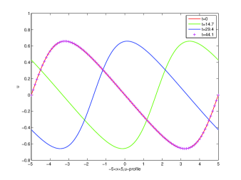
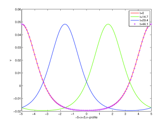
Figure 1: Profile of $u$ and $v$ of the first example of Table 1. Figure left: $u$-profile; Figure right: $v$-profile

4.2 $2$-periodic waves

In this case, the nonlinear algebraic system (2.14)-(2.15) is an over-determined system of 8 equations with 7 unknowns. In our numerical experiments, the errors of $||{\bm{H}}||_{2}=0$ also hold within $\sim 10^{-15}$. See the detailed examples in Tables 3-4 and Figs. 2-3. These waves are periodic in space but only quasi-periodic in time. We also give an example of $l_{j}=0(j=1,2)$(see the last example in Table 3).

$k_{1}$

$k_{2}$

$\tau_{11}$

$\tau_{22}$

$c_{1}^{[0]}$

$c_{2}^{[0]}$

$\omega_{1}$

$\omega_{2}$

$l_{1}$

$l_{2}$

$\tau_{12}$

$c_{1}$

$c_{2}$

$1\times\frac{2\pi}{10}$

$2\times\frac{2\pi}{10}$

$0.96\times 2\pi$

$1.23\times 2\pi$

$1$

$1$

$0.3556$

$-1.9620$

$0.0313$

$3.0793$

$0.9060$

$0.0460$

$0.0651$

$k_{1}$

$k_{2}$

$\tau_{11}$

$\tau_{22}$

$c_{1}^{[0]}$

$c_{2}^{[0]}$

$\omega_{1}$

$\omega_{2}$

$l_{1}$

$l_{2}$

$\tau_{12}$

$c_{1}$

$c_{2}$

$1\times\frac{2\pi}{10}$

$2\times\frac{2\pi}{10}$

$0.46\times 2\pi$

$1.03\times 2\pi$

$1$

$1$

$0.3724$

$-1.8403$

$0.2439$

$2.9825$

$1.0610$

$1.4268$

$0.3234$

$k_{1}$

$k_{2}$

$\tau_{11}$

$\tau_{22}$

$c_{1}^{[0]}$

$c_{2}^{[0]}$

$\omega_{1}$

$\omega_{2}$

$l_{1}$

$l_{2}$

$\tau_{12}$

$c_{1}$

$c_{2}$

$1\times\frac{2\pi}{10}$

$2\times\frac{2\pi}{10}$

$0.52\times 2\pi$

$1.13\times 2\pi$

$1$

$-1$

$-0.2612$

$-0.8778$

$0$

$0$

$-0.5938$

$0.3925$

$0$

Table 3: $2$-periodic waves: examples with $v_{0}=0$

$k_{1}$

$k_{2}$

$\tau_{11}$

$\tau_{22}$

$c_{1}^{[0]}$

$c_{2}^{[0]}$

$\omega_{1}$

$\omega_{2}$

$l_{1}$

$l_{2}$

$\tau_{12}$

$c_{1}$

$c_{2}$

$1\times\frac{2\pi}{10}$

$2\times\frac{2\pi}{10}$

$0.96\times 2\pi$

$1.23\times 2\pi$

$1$

$1$

$1.4078$

$3.3761$

$1.4515$

$1.7779$

$2.2216$

$0.6755$

$0.0575$

$k_{1}$

$k_{2}$

$\tau_{11}$

$\tau_{22}$

$c_{1}^{[0]}$

$c_{2}^{[0]}$

$\omega_{1}$

$\omega_{2}$

$l_{1}$

$l_{2}$

$\tau_{12}$

$c_{1}$

$c_{2}$

$1\times\frac{2\pi}{10}$

$2\times\frac{2\pi}{10}$

$0.46\times 2\pi$

$1.03\times 2\pi$

$1$

$1$

$1.3897$

$3.3863$

$1.9282$

$1.9582$

$1.9332$

$5.1707$

$0.9571$

$k_{1}$

$k_{2}$

$\tau_{11}$

$\tau_{22}$

$c_{1}^{[0]}$

$c_{2}^{[0]}$

$\omega_{1}$

$\omega_{2}$

$l_{1}$

$l_{2}$

$\tau_{12}$

$c_{1}$

$c_{2}$

$1\times\frac{2\pi}{10}$

$2\times\frac{2\pi}{10}$

$0.52\times 2\pi$

$1.13\times 2\pi$

$1$

$-1$

$1.3843$

$3.3920$

$1.7341$

$1.8698$

$2.0174$

$3.1582$

$0.5405$

Table 4: $2$-periodic waves: examples with $v_{0}=1$

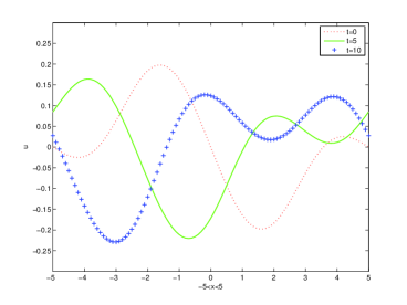
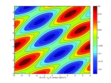
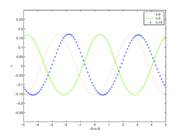
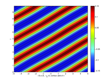
Figure 2: The first example of Table 3. Top left: $u$-profile; Top right: contour plot of $u$; Below left: $v$-profile; Below right: contour plot of $v$.

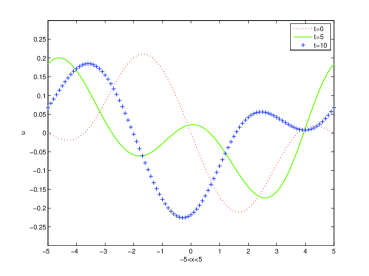
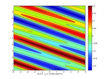
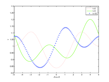
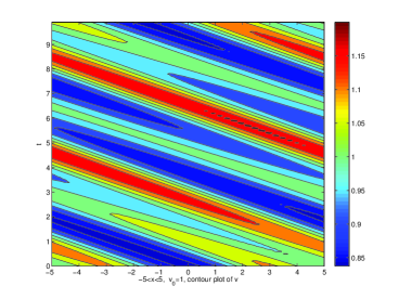
Figure 3: The first example of Table 4. Top left: $u$-profile; Top right: contour plot of $u$; Below left: $v$-profile; Below right: contour plot of $v$.

4.3 $3$-periodic waves

In the case of $3$-periodic waves, the problem is a nonlinear system of 16 equations with 11 unknowns. Some detailed numerical examples are given in Tables 5-6. As shown in Figs. 4-5, the $3$-periodic wave represents three waves interact with each other repeatedly.

In some cases, the numerical experiments will produce results with $l_{j}=0$(see the third example in Table 5). As we stated before, this kind of solutions will reduce to the solutions of the Ramani equation (4.22). However, as the iterative output ${\bm{x}}^{[j]}$ tends to the exact solution, the corresponding matrix $\bm{J}^{\mathsf{T}}\bm{J}$ will be near-singular which will result in accuracy degradation. Actually, in the third example of Table 5, the error of $||{\bm{H}}||_{2}=0$ only holds within $\sim 10^{-9}$ while in the other examples, the errors hold within $\sim 10^{-14}$.

$k_{1}$	$k_{2}$	$k_{3}$	$\tau_{11}$	$\tau_{22}$	$\tau_{33}$	$c_{1}^{[0]}$	$c_{2}^{[0]}$
$1\times\frac{2\pi}{10}$	$2\times\frac{2\pi}{10}$	$3\times\frac{2\pi}{10}$	$0.67\times 2\pi$	$0.86\times 2\pi$	$1.02\times 2\pi$	$1$	$1$
$\omega_{1}$	$\omega_{2}$	$\omega_{3}$	$l_{1}$	$l_{2}$	$l_{3}$	$\tau_{12}$	$\tau_{13}$	$\tau_{23}$	$c_{1}$	$c_{2}$
$0.4685$	$-0.8643$	$7.0815$	$-0.9501$	$1.0718$	$0.0183$	$-1.4992$	$1.0605$	$1.6167$	$24.5355$	$0.1485$
$k_{1}$	$k_{2}$	$k_{3}$	$\tau_{11}$	$\tau_{22}$	$\tau_{33}$	$c_{1}^{[0]}$	$c_{2}^{[0]}$
$1\times\frac{2\pi}{10}$	$2\times\frac{2\pi}{10}$	$3\times\frac{2\pi}{10}$	$0.46\times 2\pi$	$1.02\times 2\pi$	$1.53\times 2\pi$	$-1$	$1$
$\omega_{1}$	$\omega_{2}$	$\omega_{3}$	$l_{1}$	$l_{2}$	$l_{3}$	$\tau_{12}$	$\tau_{13}$	$\tau_{23}$	$c_{1}$	$c_{2}$
$0.1981$	$2.1281$	$-2.8105$	$0.0942$	$0.0220$	$-0.1015$	$1.5832$	$-1.1454$	$1.2599$	$3.2383$	$0.0428$
$k_{1}$	$k_{2}$	$k_{3}$	$\tau_{11}$	$\tau_{22}$	$\tau_{33}$	$c_{1}^{[0]}$	$c_{2}^{[0]}$
$1\times\frac{2\pi}{10}$	$2\times\frac{2\pi}{10}$	$3\times\frac{2\pi}{10}$	$0.53\times 2\pi$	$0.75\times 2\pi$	$1.13\times 2\pi$	$1$	$1$
$\omega_{1}$	$\omega_{2}$	$\omega_{3}$	$l_{1}$	$l_{2}$	$l_{3}$	$\tau_{12}$	$\tau_{13}$	$\tau_{23}$	$c_{1}$	$c_{2}$
$0.8089$	$-1.0065$	$-0.1976$	$0$	$0$	$0$	$-1.5390$	$1.7911$	$3.1734$	$36.8174$	$0$
$k_{1}$	$k_{2}$	$k_{3}$	$\tau_{11}$	$\tau_{22}$	$\tau_{33}$	$c_{1}^{[0]}$	$c_{2}^{[0]}$
$1\times\frac{2\pi}{10}$	$2\times\frac{2\pi}{10}$	$3\times\frac{2\pi}{10}$	$0.53\times 2\pi$	$0.75\times 2\pi$	$1.13\times 2\pi$	$-1$	$1$
$\omega_{1}$	$\omega_{2}$	$\omega_{3}$	$l_{1}$	$l_{2}$	$l_{3}$	$\tau_{12}$	$\tau_{13}$	$\tau_{23}$	$c_{1}$	$c_{2}$
$0.5147$	$1.6120$	$-2.7811$	$-0.7670$	$-0.1002$	$0.8148$	$1.7865$	$-1.6037$	$1.2270$	$23.1536$	$-0.1155$

Table 5: $3$-periodic waves: examples with $v_{0}=0$

$k_{1}$	$k_{2}$	$k_{3}$	$\tau_{11}$	$\tau_{22}$	$\tau_{33}$	$c_{1}^{[0]}$	$c_{2}^{[0]}$
$1\times\frac{2\pi}{10}$	$2\times\frac{2\pi}{10}$	$3\times\frac{2\pi}{10}$	$0.67\times 2\pi$	$0.86\times 2\pi$	$1.02\times 2\pi$	$1$	$1$
$\omega_{1}$	$\omega_{2}$	$\omega_{3}$	$l_{1}$	$l_{2}$	$l_{3}$	$\tau_{12}$	$\tau_{13}$	$\tau_{23}$	$c_{1}$	$c_{2}$
$1.4388$	$3.1394$	$7.9404$	$1.6866$	$2.0555$	$1.5475$	$2.1251$	$1.2939$	$2.7630$	$24.0624$	$0.9121$
$k_{1}$	$k_{2}$	$k_{3}$	$\tau_{11}$	$\tau_{22}$	$\tau_{33}$	$c_{1}^{[0]}$	$c_{2}^{[0]}$
$1\times\frac{2\pi}{10}$	$2\times\frac{2\pi}{10}$	$3\times\frac{2\pi}{10}$	$0.46\times 2\pi$	$1.02\times 2\pi$	$1.53\times 2\pi$	$-1$	$1$
$\omega_{1}$	$\omega_{2}$	$\omega_{3}$	$l_{1}$	$l_{2}$	$l_{3}$	$\tau_{12}$	$\tau_{13}$	$\tau_{23}$	$c_{1}$	$c_{2}$
$1.3915$	$3.3788$	$8.3344$	$1.9342$	$1.9653$	$1.5315$	$1.9341$	$1.2573$	$2.8808$	$6.0244$	$0.9791$
$k_{1}$	$k_{2}$	$k_{3}$	$\tau_{11}$	$\tau_{22}$	$\tau_{33}$	$c_{1}^{[0]}$	$c_{2}^{[0]}$
$1\times\frac{2\pi}{10}$	$2\times\frac{2\pi}{10}$	$3\times\frac{2\pi}{10}$	$0.53\times 2\pi$	$0.75\times 2\pi$	$1.13\times 2\pi$	$-1$	$1$
$\omega_{1}$	$\omega_{2}$	$\omega_{3}$	$l_{1}$	$l_{2}$	$l_{3}$	$\tau_{12}$	$\tau_{13}$	$\tau_{23}$	$c_{1}$	$c_{2}$
$1.3608$	$2.4234$	$-3.9766$	$1.7988$	$2.3352$	$1.0781$	$2.0257$	$-1.9751$	$0.6098$	$44.3977$	$2.6950$

Table 6: $3$-periodic waves: examples with $v_{0}=1$

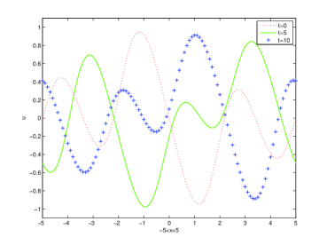
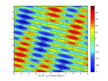
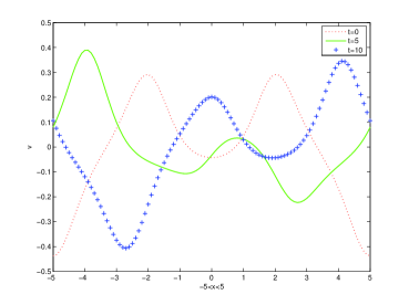
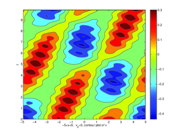
Figure 4: The first example of Table 5. Top left: $u$-profile; Top right: contour plot of $u$; Below left: $v$-profile; Below right: contour plot of $v$.

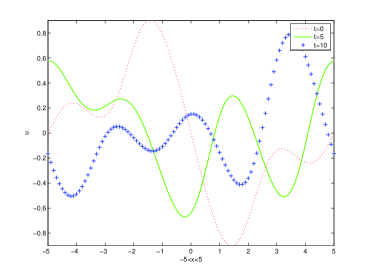
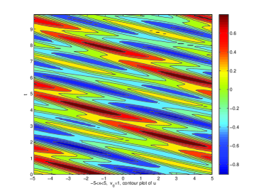
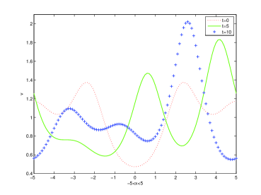
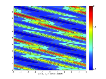
Figure 5: The first example of Table 6. Top left: $u$-profile; Top right: contour plot of $u$; Below left: $v$-profile; Below right: contour plot of $v$.

5 Conclusion and discussion

A numerical process of calculating $N$-periodic waves is presented and some numerical experiments are carried out with the coupled Ramani equation. The numerical results show that the process is efficient in calculating $1$-, $2$- and $3$-periodic waves. Here we give two remarks.

Firstly, the numerical results are not unique since this is a nonlinear and over-determined system. For instance, in the third and forth examples in Table 5, with the same given parameters but the different initial guess, we obtain two different $3$-periodic waves.

Secondly, there are many other soliton equations that can be transformed into the coupled bilinear KdV-type systems. For instance, the Hirota-Satsuma coupled KdV equation[32]

$$u_{t}=\frac{1}{4}u_{xxx}+3uu_{x}+3(-\phi^{2}+\omega)_{x},$$ (5.24)

$$\phi_{t}=-\frac{1}{2}\phi_{xxx}-3u\phi_{x},$$ (5.25)

$$\omega_{t}=\frac{1}{2}\omega_{xxx}-3u\omega_{x}.$$ (5.26)

can be transformed into the bilinear form

$$(D_{x}D_{t}-\frac{1}{4}D_{x}^{4}-\frac{3}{4}D_{z}^{2})f\cdot f=0,$$ (5.27)

$$D_{z}(D_{t}+\frac{1}{2}D_{x}^{3})f\cdot f=0,$$ (5.28)

by the dependent variable transformation

$$u=(\mathrm{ln}f)_{xx},\quad\phi=\frac{1}{2}\frac{f_{z}}{f},\quad\omega=\frac{1}{2}\frac{f_{zz}}{f}$$ (5.29)

where $z$ is an auxiliary variable, and the Camassa-Holm equation[33, 34]

$$u_{t}+2\kappa^{2}u_{x}+3uu_{x}-u_{xxt}=2u_{x}u_{x}x+uu_{xxx},$$ (5.30)

can be transformed into

$$[D_{y}(D_{t}+2\kappa^{3}D_{y}-\kappa^{2}D_{y}^{2}D_{t})$$

$$\qquad\qquad\qquad+\frac{1}{3}\kappa^{2}D_{t}(D_{\tau}+D_{y}^{3})]f\cdot f=0,$$ (5.31)

$$D_{y}(D_{\tau}+D_{y}^{3})f\cdot f=0.$$ (5.32)

with a so-called reciprocal transformation. Here $\tau$ is an auxiliary variable and coordinate $(y,t)$ is generated from the reciprocal transformation. See details in Ref. [34].

Some discrete systems can also be transformed into this kind of bilinear equations. For example, the semi-discrete KdV equation given by Hirota and Ohta [35],

$$\frac{4}{1+a^{2}u_{n}}\frac{d}{dt}u_{n}=\Delta^{3}Mu_{n}+6u_{n}\Delta Mu_{n}$$

$$\qquad\qquad+a^{2}[\Delta M(u_{n}\Delta^{2}u_{n})+3(\Delta Mu_{n})(\Delta^{2}u_{n})],$$ (5.33)

can be transformed into

$$[2aD_{z}\sinh(\frac{D_{n}}{2})-\cosh(\frac{3D_{n}}{2})+\cosh(\frac{D_{n}}{2})]f\cdot f=0,$$

(5.34)

$$(4a^{2}D_{t}+3D_{z})\sinh(\frac{D_{n}}{2})f\cdot f=D_{z}\sinh(\frac{3D_{n}}{2})f\cdot f,$$ (5.35)

with transformation

$$u_{n}=\frac{1}{a^{2}}(\frac{f_{n+2}f_{n-1}}{f_{n+1}f_{n}}-1).$$ (5.36)

Our numerical process may also be applied to these soliton equations to study their $N$-periodic wave solutions if some additional terms with arbitrary integral constants are introduced in these bilinear forms.

References

- [1] R. Hirota, The direct method in soliton theory, Cambridge University Press, 2004.
- [2] S. P. Novikov, A periodic problem for the Korteweg-de Vries equation, I. Funktsional Anal. i Prilozhen., 8(3):54-66, 1974.
- [3] B. A. Dubrovin, Periodic problems for the Korteweg-deVries equation in the class of finite band potentials, Funct. Anal. Appl., 9(3):215-223, 1975.
- [4] B. A. Dubrovin and S. P. Novikov, Periodic and conditionally periodic analogues of the many-soliton solutions of the Kortweg-deVries equation, Sov. Phys. JETP, 40:1058, 1975.
- [5] P. D. Lax, Periodic solutions of the KdV equation, Comm. Pure Appl. Math., 28:141-188, 1975.
- [6] A. R. Its and V. B. Matveev, The periodic Korteweg-deVries equation, Funct. Anal. Appl., 9(1):67, 1975.
- [7] H. P. McKean and P. van Moerbeke, The spectrum of Hill’s equation, Inv. Math., 30(3):217-274, 1975.
- [8] Y. C. Ma and M. J. Ablowitz, The periodic cubic Schrödinger equation, Stud Appl. Math., 65:113, 1981.
- [9] M. G. Forest and D. W. McLaughlin, Spectral theory for the periodic sine-Gordon equation: A concrete viewpoint, J. Math. Phys. 23:1248, 1982.
- [10] E. Date and S. Tanaka, Periodic multi-soliton solutions of Korteweg-de Vries equation and Toda lattice, Suppl. Prog. Theor. Phys., 59:107-126, 1976.
- [11] I. M. Krichever, Algebraic-geometric construction of the Zaharov-Sabat equations and their periodic solutions, Dokl. Akad. Nauk SSSR, 227:394-397, 1976.
- [12] B. A. Dubrovin, Theta functions and nonlinear equations, Russ. Math. Surv., 36:11-92, 1981.
- [13] E. D. Belokolos, A. I. Bobenko, V. Z. Enol’skii, A. R. Its, and V. B. Matveev, Algebro-Geometric Approach to Nonlinear Integrable Equations, Springer-Verlag, Berlin,1994.
- [14] C. W. Cao, Y.T. Wu and X.G. Geng, On quasi-periodic solutions of the 2+1 dimensional Caudrey-Dodd-Gibbon-Kotera-Sawada equation, Physics Letters A, 256(1):59-65, 1999.
- [15] X. G. Geng, L. H. Wu and G. L. He, Quasi-periodic solutions of the Kaup-Kupershmidt hierarchy, Journal of Nonlinear Science, 23(4): 527-555, 2013.
- [16] X. G. Geng, L. H. Wu and G. L. He, Algebro-geometric constructions of the modified Boussinesq flows and quasi-periodic solutions, Physica D: Nonlinear Phenomena,240(16):1262-1288, 2011.
- [17] X. G. Geng, L. H. Wu and G. L. He, Quasi-Periodic Solutions of Nonlinear Evolution Equations Associated with a 3 3 Matrix Spectral Problem. Studies in Applied Mathematics, 127(2):107-140, 2011.
- [18] A. Nakamura, A direct method of calculating periodic wave solutions to nonlinear evolution equations. I. Exact two-periodic wave solution, Journal of the Physical Society of Japan, 47(5): 1701-1705, 1979.
- [19] A. Nakamura, A Direct Method of Calculating Periodic Wave Solutions to Nonlinear Evolution Equations. II. Exact One- and Two-Periodic Wave Solution of the Coupled Bilinear Equations, Journal of the Physical Society of Japan, 48(4):1365-1370, 1980.
- [20] R. Hirota and M. Ito, A Direct Approach to Multi-Periodic Wave Solutions to Nonlinear Evolution Equations, Journal of the Physical Society of Japan, 50(1):338-342, 1981.
- [21] W. X. Ma and E. G. Fan, Linear superposition principle applying to Hirota bilinear equations, Computers Mathematics with Applications, 61(4):950-959, 2011.
- [22] L. Luo and E. G. Fan, Bilinear approach to the quasi-periodic wave solutions of Modified Nizhnik-Novikov-Vesselov equation in (2+1) dimensions, Physics Letters A, 374(30):3001-3006, 2010.
- [23] E. G. Fan, K. W. Chow and J. H. Li, On doubly periodic standing wave solutions of the coupled Higgs field equation. Studies in Applied Mathematics, 128(1):86-105, 2012.
- [24] T. Trogdon and B. Deconinck, Numerical computation of the finite-genus solutions of the Korteweg-de Vries equation via Riemann-Hilbert problems, Appl. Math. Lett., 26:5-9, 2013.
- [25] T. Trogdon and B. Deconinck, A numerical dressing method for the nonlinear superposition of solutions of the KdV equation, Nonlinearity, 27:67-86, 2014.
- [26] J. Frauendiener and C. Klein, Hyperelliptic theta-functions and spectral methods, Journal of Computational and Applied Mathematics, 167: 193-218, 2004.
- [27] J. Frauendiener and C. Klein, Hyperelliptic theta-Functions and spectral methods: KdV and KP Solutions, Letters in Mathematical Physics, 76:249-267, 2006.
- [28] C. Kalla and C. Klein, On the numerical evaluation of algebro-geometric solutions to integrable equations, Nonlinearity, 25:569-596, 2012.
- [29] A. Osborne, Nonlinear Ocean Waves the Inverse Scattering Transform. Academic Press, 2010.
- [30] A. Ramani, Inverse scattering, ordinary differential equations of Painlev-type, and Hirota’s bilinear formalism, Annals of the New York Academy of Sciences, 373(1): 54-67, 1981.
- [31] X.B. Hu and D.L. Wang, Lax pairs and Bäcklund transformations for a coupled Ramani equation and its related system, Appl. Math. Lett., 13:45-48, 2000.
- [32] J. Satsuma and R. Hirota, A coupled KdV equation is one case of the four-reduction of the KP hierarchy, Journal of the Physical Society of Japan, 51(10): 3390-3397, 1982.
- [33] R. Camassa and D.D. Holm, An integrable shallow water equation with peaked solitons, Physical Review Letters, 71(11): 1661, 1993.
- [34] A. Parker, On the Camassa-Holm equation and a direct method of solution I. Bilinear form and solitary waves, Proceedings of the Royal Society of London A: Mathematical, Physical and Engineering Sciences, 460(2050): 2929-2957, 2004.
- [35] Y. Ohta and R. Hirota, A discrete KdV equation and its Casorati determinant solution, Journal of the Physical Society of Japan, 60(6): 2095-2095, 1991.
- [36] Y.N. Zhang, H.W. Tam and X.B. Hu, Integrable discretization of “time” and its application on the Fourier pseudospectral method to the Korteweg-de Vries equation, Journal of Physics A: Mathematical and Theoretical, 47(4): 045202, 2014.
- [37] Y.N. Zhang, X.B. Hu and H.W. Tam, Integrable discretization of nonlinear Schrödinger equation and its application with Fourier pseudo-spectral method. Numerical Algorithms, 69(4): 839-862, 2015.
- [38] J.X. Zhao and H.W. Tam, Soliton solutions of a coupled Ramani equation, Appl. Math. Lett, 19:307-313, 2006.
- [39] A.M. Wazwaz and H. Triki, Multiple soliton solutions for the sixth-order Ramani equation and a coupled Ramani equation, Applied Mathematics and Computation, 216(1): 332-336, 2010.
- [40] A.M. Wazwaz, Multiple soliton solutions for a new coupled Ramani equation, Physica Scripta, 83(1): 015002, 2010.
- [41] J. Chen, B.F.Feng and Y. Chen, Bilinear Bäcklund transformation, Lax pair and multi-soliton solution for a vector Ramani equation, Modern Physics Letters B, 31(12): 1750133, 2017.
- [42] N. Li and B. Gao, Hamiltonian structures of a coupled Ramani equation, J. Math. Anal. Appl. 453:908-916, 2017.
- [43] A. Björck, Numerical methods for least squares problems, SIAM, 1996.