Path integral Monte Carlo simulations of dense carbon-hydrogen plasmas

Abstract

Carbon-hydrogen plasmas and hydrocarbon materials are of broad interest to laser shock experimentalists, high energy density physicists, and astrophysicists. Accurate equations of state (EOS) of hydrocarbons are valuable for various studies from inertial confinement fusion (ICF) to planetary science. By combining path integral Monte Carlo (PIMC) results at high temperatures and density functional theory molecular dynamics (DFT-MD) results at lower temperatures, we compute the EOS for hydrocarbons from simulations performed at 1473 separate ($\rho,T$)-points distributed over a range of compositions. These methods accurately treat electronic excitation effects with no adjustable parameter nor experimental input. PIMC is also an accurate simulation method that is capable of treating many-body interaction and nuclear quantum effects at finite temperatures. These methods therefore provide a benchmark-quality EOS that surpasses that of semi-empirical and Thomas-Fermi-based methods in the warm dense matter regime. By comparing our first-principles EOS to the LEOS 5112 model for CH, we validate the specific heat assumptions in this model but suggest that the Grüneisen parameter is too large at low temperature. Based on our first-principles EOS, we predict the principal Hugoniot curve of polystyrene to be 2-5$\%$ softer at maximum shock compression than that predicted by orbital-free DFT and SESAME 7593. By investigating the atomic structure and chemical bonding of hydrocarbons, we show a drastic decrease in the lifetime of chemical bonds in the pressure interval from 0.4 to 4 megabar. We find the assumption of linear mixing to be valid for describing the EOS and the shock Hugoniot curve of hydrocarbons in the regime of partially ionized atomic liquids. We make predictions of the shock compression of glow-discharge polymers and investigate the effects of oxygen content and C:H ratio on its Hugoniot curve. Our full suite of first-principles simulation results may be used to benchmark future theoretical investigations pertaining to hydrocarbon EOS, and should be helpful in guiding the design of future experiments on hydrocarbons in the gigabar regime.

I Introduction

Accurate equations of state (EOS) of materials under various temperature and pressure conditions is of fundamental importance in earth and planetary science, astrophysics, and high energy density physics. Tang et al. (2017) These applications require that we understand matter that is partially ionized and strongly coupled. This includes conventional condensed matter ($T\ll T_{\rm Fermi}$), warm dense matter ($T\sim T_{\rm Fermi}$), and weakly coupled plasmas ($T\gg T_{\rm Fermi}$ and $\langle$potential energy$\rangle\ll\langle$kinetic energy$\rangle$). At high temperatures ($>$10² eV) and near-ambient densities, electrons and nuclei can generally both be treated as ideal gases, due to complete ionization of atoms into a perfect plasma state. At slightly lower temperatures, the Debye-Hückel model may be used to treat weak interactions within a screening approximation. Materials in condensed forms are characterized by both strong coupling and degeneracy effects and thus require sophisticated quantum many-body methods for their description. However, very good progress can be made with average-atom methods such as average-atom Thomas-Fermi theory and average-atom Kohn-Sham Density Functional Theory (DFT), in which isolated ions are embedded within a spherically-symmetric electron liquid. Kohn-Sham-DFT average-atom methods resolve distinct electronic shells of atoms, just as in conventional applications of quantum theory to isolated atoms, but they do not account for directional bonding between atoms and therefore fail at low temperatures. Thomas-Fermi and more general orbital-free (OF) DFT approaches do not account for electronic shell effects and are thus unable to properly describe partially ionized plasmas; as such, they provide a less than satisfactory description of warm dense matter.

EOS models (e.g., of the QEOS type More et al. (1988)) treating wide ranges of density and temperature and databases that house them (e.g., SESAME Lyon and Johnson (1992) and LEOS), make heavy use of average-atom theories for electronic excitations, ad hoc interpolation formulas which mediate the evolution of the ionic specific heat from low-$T$ to the high-$T$ ideal gas limit, and semi-empirical models which allow for the fitting of experimental results near ambient conditions. The efficacy of these EOS models is questionable precisely in the regimes currently probed in dynamic compression experiments reaching gigabar (Gbar) pressures, in which it is expected that atoms are significantly (though not fully) ionized by both temperature and pressure. Clearly, this regime is in need of more sophisticated theoretical treatments which more fully account for detailed electronic structure and many-body effects.

First-principles molecular dynamics (MD) based on DFT is widely used for calculating the atomic structure, the EOS, and other electronic and ionic properties of materials at relatively low temperatures, where the ionization fraction is small. In DFT-MD, the nuclei are usually treated as classical particles whose motion follows Newton’s equation of motion, whereas the potential field is determined by solving a single-particle mean-field equation self-consistently using DFT. This method naturally includes the anharmonic terms of nuclear vibrations and is usually a good approximation for systems with heavy elements, and is widely used for simulations of earth and planetary materials Wilson and Militzer (2010, 2012); Wilson, Wong, and Militzer (2013); Wahl and Militzer (2015); Zhang et al. (2016a); Soubiran et al. (2017). For light elements, zero-point motion cannot be neglected Morales et al. (2013a, b), which makes important contributions to the energy that may alter relative phase stability. At temperatures above 100 eV, DFT-MD of the Kohn-Sham variety becomes computationally intractable due to the considerable number of high-lying single-electron states that need to be included. It is also practically limited by the use of pseudopotentials that reduce computational costs by freezing inner-shell electrons within ionic cores that tend to overlap between neighboring atoms if the system is at significant compression, leading to errors.

Path integral Monte Carlo (PIMC) D. M. Ceperley (1995); Ceperley (1996) offers an approach to directly solve the many-body Schrödinger equation in a stochastic way. It typically treats nuclei and electrons as quantum paths that evolve in imaginary time, and obtains the energy and other properties of a system by solving for the thermal density matrix and computing thermodynamic averages within the sampled ensembles. For Fermionic systems, a suitable nodal structure is required to restrict the sampling space in order to avoid the sign problem that arises from antisymmetry of the many-body density matrix. Accuracy of the method has been demonstrated by early work on fully-ionized hydrogen Pierleoni et al. (1994); Militzer and Ceperley (2001) and helium Militzer (2009) plasmas. In the past five years, developments by extending free-particle nodes Driver and Militzer (2012) or implementing localized orbitals Militzer and Driver (2015a) to construct the nodes have enabled PIMC studies of a series of heavier elements and compounds Driver and Militzer (2012); Benedict et al. (2014); Driver and Militzer (2015); Militzer and Driver (2015b); Driver et al. (2015); Militzer and Driver (2015a); Driver and Militzer (2016); Hu et al. (2016a); Zhang et al. (2016b); Driver et al. (2017); Driver and Militzer (2017); Zhang et al. (2017a, b). These works have applied PIMC to EOS calculations at temperatures ranging from a few hundred million K to as low as 2.5$\times 10^{5}$ K. For first- and second-row elements, PIMC and DFT-MD simulations produce consistent EOS results at intermediate temperatures.

While computer simulations with classical nuclei provide sufficiently accurate predictions for a wide range of thermodynamic conditions, at low temperature, nuclear quantum effects (NQEs) often play an important role in predicting observed phenomena Cazorla and Boronat (2017). One typically compares the inter-particle spacing to the thermal de Broglie wavelength ($\sim 1/\sqrt{mk_{\rm B}T}$) that is inversely proportional to the square root of mass and temperature, and, therefore cold and low-Z materials are strongly influenced by NQE. Often such effects are referred to as zero point motion. In solids, zero point effects are typically studied with lattice dynamics calculations that derive the spectrum of vibrational eigenmodes within the quasi-harmonic approximation. Such calculations rely on the second derivative the energy with respect to the nuclear positions that can be derived with theoretical methods of various levels of accuracy ranging from classical force fields Rappé et al. (1992), DFT Gonze and Lee (1997); Baroni et al. (2001), and in principle also with quantum Monte Carlo calculations Foulkes et al. (2001). It is difficult, however, to introduce anharmonic effects accurately into the lattice dynamics approach Zhou et al. (2014). Anharmonic effects are important for temperatures above the Debye temperature, in particular near melting, but also at very low temperature in materials that are rich in hydrogen or helium. Because of their small mass, the nuclear wavefunctions often spread into the anharmonic regions of the confining potential even in the ground state so that anharmonic effects can no longer be neglected.

Path integral methods Feynman (1972) can accurately incorporate NQE and anharmonic effects at all temperatures and can describe solids as well as liquids Jones and Ceperley (1996); Militzer and Graham (2006). An efficient approach, that has been devised to pursue NQE problems, is to combine the path integral method for nuclei with other electronic structure methods, such as DFT or quantum Monte Carlo, to efficiently describe the forces between the nuclei. Path integral molecular dynamics Oh and Deymier (1998) and coupled electron ion Monte Carlo Pierleoni and Ceperley (2006) are two common techniques that employ this combined approach Graziani et al. (2014). A few examples include transport properties Kang et al. (2014) and phase transitions in solid McMahon et al. (2012); Morales et al. (2013b) and liquid Morales et al. (2010, 2013a); Pierleoni et al. (2016) hydrogen, helium Pollock and Ceperley (1984); Militzer (2009), hydrogen-bonding in water Chen et al. (2003); Morrone and Car (2008); Li, Walker, and Michaelides (2011); Ceriotti et al. (2016) and on metal surfaces Li et al. (2010), solid water-ice phases Benoit, Marx, and Parrinello (1998); Pamuk et al. (2012), phonon dispersion in diamond Ramírez, Herrero, and Hernández (2006) and energy barriers for small molecules Weht et al. (1998); Hauser, Mitrushchenkov, and de Lara-Castells (2017).

In this work, we employ the path integral methods to study partially and highly excited electrons. Even though the temperatures under consideration are quite high ($\sim$100 eV), fermionic effects are crucial to characterize the electronic states accurately. The occupation of bound electronic states affects the motion of the nuclei through Pauli exclusion. At high density, the motion of the nuclei deforms the shape of the electronic orbitals. Thus, a fully self-consistent approach is needed for materials in the WDM regime.

We apply PIMC simulations with free-particle nodes and DFT-MD calculations to study carbon-hydrogen compounds. Hydrocarbons are currently in use as ablator materials in dynamic compression and inertial confinement fusion (ICF) experiments Betti and Hurricane (2016); Meezan et al. (2016); Goncharov et al. (2016); Guillot (2005); Wallerstein et al. (1997). Materials such as polystyrene and glow-discharge polymer (GDP) have been a strong point of interest and extensively studied by both theorists and experimentalists Hauver and Melani (1964); Dudoladov et al. (1969); Lamberson, Asay, and Guenther (1972); Marsh (1980); Nellis et al. (1984); Kodama et al. (1991); Bushman et al. (1996); Koenig et al. (1998); Cauble et al. (1997, 1998); Koenig et al. (2003); Ozaki et al. (2005); Hu et al. (2008); Ozaki et al. (2009); Barrios et al. (2010); Shu et al. (2010); Shang et al. (2013); Shu et al. (2015); Barrios et al. (2012); Huser et al. (2013, 2015); Moore et al. (2016); Hamel et al. (2012). Recently, laser shock experiments at the National Ignition Facility (NIF) Kraus et al. (2016); Swift et al. (2012); Döppner et al. (2014); Kritcher et al. (2014, 2016); Nilsen et al. (2016) and the OMEGA Laser facility Nora et al. (2015) have extended the ablation pressure in CH to the Gbar range CHG . Calculations employing DFT-MD or OF-DFT have been performed to study the EOS of hydrocarbon materials Mattsson et al. (2010); Wang, He, and Zhang (2011); Lambert and Recoules (2012); Hu et al. (2014, 2015, 2016b); Huser et al. (2015); Colin-Lalu et al. (2016). These theoretical studies predicted shock Hugoniot curves that agree well with experiments at low temperatures. At high temperatures, Kohn-Sham DFT is unfeasible while OF-DFT works efficiently but its predictions are yet to be tested by other theories Hu et al. (2016a) and experiments. We expect the PIMC and DFT-MD simulations of this study to produce predictions for the EOS of hydrocarbons which are sufficiently accurate to be used as benchmarks for both the construction of wide-range EOS models, and the further investigation of hydrocarbon EOS with less computationally expensive simulation methods. Ultimately, our predictions may prove useful for the design and interpretation of dynamic compression and ICF experiments in the future.

The paper is organized as follows: Section II introduces the details of our simulation methods. Sec. III presents our EOS results, the shock Hugoniot curves, and comparisons with other theories, models, and experiments. Sec. IV discusses the structural evolution of hydrocarbons and the shock compression of GDP and related materials. We conclude in Sec. V.

II Simulation methods

We use the CUPID code Militzer (2000) for our PIMC simulations within the fixed-node approximation Ceperley (1991). We treat the nuclei as quantum particles, even though the kinetic energy is much larger than the zero-point contribution to the total energy of the system at the high temperatures ($T\geq 10^{6}$ K = 87 eV) considered here. Electrons are treated as fermions. Their quantum paths are periodic in the imaginary time interval, $0\leq t\leq\beta=1/k_{\text{B}}T$ ($k_{\text{B}}$ is the Boltzmann constant), but the paths of electrons with the same spin may be permuted as long as they do not violate the nodal restriction Ceperley (1991). Following our previous work on hydrogen Pierleoni et al. (1994); Magro et al. (1996); Militzer and Ceperley (2001); Militzer et al. (2001); Hu et al. (2010); Militzer and Ceperley (2000); Hu et al. (2011); Militzer, Magro, and Ceperley (1999); Militzer and Graham (2006), helium Militzer (2006, 2005), and carbon Driver and Militzer (2012); Benedict et al. (2014), we use free-particle nodes to constrain the sampling space by restricting the paths to positive regions of the density matrix of ideal fermions. Coulomb interactions between all pairs of particles are introduced via pair density matrices Natoli and Ceperley (1995); Militzer (2016). The pair density matrices are evaluated at an imaginary time interval of 1/1024 Hartree^-1 (Ha^-1) while the nodal restriction is enforced in steps of 1/8192 Ha^-1.

For DFT-MD simulations, we use the Vienna Ab initio Simulation Package (VASP) Kresse and Furthmüller (1996). We choose the hardest available projected augmented wave (PAW) pseudopotentials Blöchl, Jepsen, and Andersen (1994) with core radii of 1.1 and 0.8 Bohr for C and H, respectively. All electrons are treated as valence electrons. Exchange-correlation effects are treated within the local density approximation (LDA) Ceperley and Alder (1980); Perdew and Zunger (1981). We choose a large plane-wave basis cutoff of 2000 eV, the $\Gamma$ point to sample the Brillouin zone, and an MD time step of 0.05-0.2 fs, depending on the temperature. MD trajectories are generated in an $NVT$ ensemble, and typically consist 2000-10000 steps to make sure the system is in equilibrium and the energies and pressures are converged. The temperature is controlled with a Nosé thermostat Nosé (1984). All VASP energies are shifted by -37.4243 Ha/C and -0.445893 Ha/H, to put DFT-MD energies on the same scale as our all-electron PIMC energies. These values are determined by performing all-electron single-atom calculations using the OPIUM code opi .

We study six different compositions by simulating C₂₀H₁₀, C₁₈H₁₈, C₁₆H₂₄, C₁₄H₂₈, C₁₂H₃₆, and C₁₀H₄₀ in a cubic cell at temperatures between 10⁶-1.3$\times 10^{8}$ K using PIMC and 6.7$\times 10^{3}$-10⁶ K using DFT-MD methods. For C:H=1:1, we use larger cells with four times as many atoms at the lower temperatures of 6.7$\times 10^{3}$-2.5$\times 10^{5}$ K in order to minimize finite-size effects, which are expected to be larger at low temperatures Driver and Militzer (2012). In order to maximize the computational efficiency of the large-cell simulations, we freeze the 1s² electrons of carbon in the pseudopotential core without losing accuracy, because the temperatures are much lower than the ionization energy (392 eV for 1s² of C) Kramida et al. (2015). We consider a grid of nine isochores for each hydrocarbon system, chosen so that the pressure ranges for each composition are similar; this results in densities for CH between (2 - 12)$\times$$\rho_{\text{ambient}}$ (see Fig. 1). These conditions are both relevant to dynamic compression experiments, and well within the range in which Kohn-Sham DFT-MD simulations with pseudopotentials are feasible.

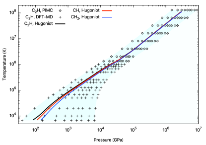
Figure 1: Pressure-temperature conditions considered in our PIMC and DFT-MD simulations of hydrocarbons. For clarity, only the EOS data for C₂H and the Hugoniot curves of C₂H, CH, and CH₂ are shown. The Hugoniot curves are obtained by setting the initial denstity to 1.12, 1.05, and 0.946 g/cm³ for C₂H, CH, and CH₂, respectively. The shaded region denotes the approximate area that the EOS of all hydrocarbons studied in this work fall in.

We also investigate the validity of the linear mixing approximation for estimating the EOS of various hydrogen-carbon mixtures. In this method, the energy and the density of the mixture are obtained with the isobaric, isothermal additive volume assumption via $V_{\rm mix}(P,T)=f_{\rm C}V_{\rm C}(P,T)+f_{\rm H}V_{\rm H}(P,T)$ and $E_{\rm mix}(P,T)=f_{\rm C}E_{\rm C}(P,T)+f_{\rm H}E_{\rm H}(P,T)$, where $f_{\rm C}=n_{\rm C}/(n_{\rm C}+n_{\rm H})$ and $f_{\rm H}=n_{\rm H}/(n_{\rm C}+n_{\rm H})$ are the mixing ratios, $V_{\rm mix}$, $V_{\rm C}$, $V_{\rm H}$ are volumes per atom for the mixture, pure carbon, and pure hydrogen respectively (and likewise for the internal energies, $E$). $E(T,P)$ and $V(T,P)$ of the pure species are constructed using bi-variable spline fitting over the $\rho$-$T$ space spanned by the EOS of pure hydrogen and pure carbon. The shock Hugoniot curves derived with simulations of the fully interacting system can be compared to that obtained with the linear mixing approximation.

III Results

III.1 Equation of state

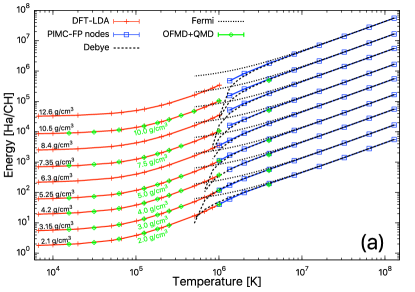
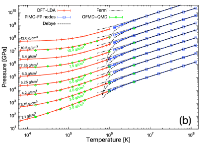
Figure 2: Internal energies and pressures of CH along isochores. Corresponding results of the Fermi-gas and the Debye-Hückel theories are plotted for comparison. PIMC predicts consistent results with DFT-MD at 10⁶ K PIMC and agrees with ideal Fermi gas and Debye-Hückel models at above 8$\times$10⁶ K. As temperature decreases, the ideal Fermi gas model significantly overestimates the energy and the pressure because of the neglect of interactions. Debye-Hückel model improves over the Fermi-gas model for temperatures down to 3$\times$10⁶ K but leads to low pressures and energies at lower temperatures, at which electron-nucleus coupling gets stronger and the screening approximation breaks down. DFT-MD and OF-DFT results from Ref. Hu et al., 2015 are shown with green diamonds for comparison. Error bars of the data are much smaller than the size of the symbols. Different isochores have been shifted apart for clarity.

Figure 2 shows the calculated EOS for C₂H along nine isochores. A complete list of EOS data for all hydrocarbons (C₂H, CH, C₂H₃, CH₂, CH₃, CH₄) in this study are in the supplementary material. The internal energies and pressures from PIMC calculations agree with predictions of the Debye-Hückel model at temperatures above 4$\times 10^{6}$ K and with the Fermi electron gas theory (wherein both ions and electrons are treated as uniform-density free Fermi gases) above 8$\times 10^{6}$ K, which is higher than the 1s¹ ionization energy (489.99 eV or 5.7$\times 10^{6}$ K) Kramida et al. (2015) of carbon. PIMC results show excellent agreement with DFT-MD at 10⁶ K, with differences typically less than 1 Ha/carbon in internal energy and 3% in pressure. We have therefore constructed a consistent first-principles EOS table for warm dense hydrocarbons, over a wide density-temperature range of 1.4-13.5 g/cm³ and $6.7\times 10^{3}$-$1.3\times 10^{8}$ K and C:H=2:1-1:4. The good consistency of PIMC with DFT-MD and the other high-temperature theories indicates it is reliable to use the free-particle nodes in PIMC for temperatures as low as $10^{6}$ K, and PAW pseudopotentials and zero-temperature exchange-correlation functionals in DFT-MD up to $10^{6}$ K.

In comparison with a recent first-principles study Hu et al. (2015) that employs DFT-MD with the Perdew-Burke-Ernzerhof (PBE) Perdew, Burke, and Ernzerhof (1996) exchange-correlation functional at temperatures below the Fermi temperature $T_{\rm Fermi}$, the $P$-$T$ and $E$-$T$ curves coincide with LDA curves in this work. This indicates the EOS does not significantly depend on the form of the exchange-correlation functional in the temperature interval under consideration. At $10^{6}$ K and higher temperatures, the energy of Ref. Hu et al., 2015 is different from PIMC predictions of this work while the pressure differences are small. This is associated with underestimation of the compression maximum by OF-DFT that is used in Ref. Hu et al., 2015. More details on this will be discussed in Sec. III.3.

III.2 Comparisons with the LEOS-5112 model for CH

An important aim of this work is to produce benchmarking EOS predictions that will act as constraints in the future construction of EOS models for hydrocarbons which span wide ranges of density and temperature, well beyond that where experimental data is available. It is therefore interesting to compare the details of existing EOS models for, e.g., CH to the first-principles predictions in this work. The most recent such model for polystyrene (CH) constructed at the Lawrence Livermore National Laboratory is LEOS-5112, closely related to LEOS-5400 Sterne et al. (2016), currently used as the EOS model of choice for GDP in inertial confinement fusion simulations where that material is employed as an ablator. EOS models such as these assume that the free energy is decomposable into separate ionic and electronic excitation terms. While somewhat justified due to the large ion/electron mass ratio, it is important whenever possible to compare to EOS predictions from ab initio methods (such as PIMC) that do not make this assumption.

The LEOS-5400 EOS model Sterne et al. (2016) was originally constructed to represent the non-stoichiometric carbon-hydrogen-oxygen composition of GDP, and to reproduce both Hugoniot and off-Hugoniot measurements (specifically, shock-and-release from an interface with deuterium) Hamel et al. (2012). More recently, LEOS-5112 was developed to facilitate comparison with experiments and simulations on the stoichiometric material, CH. This CH model closely follows the parameters used to make GDP LEOS-5400.

The cold curve, $E(V,T=0)$, was based on a constant-pressure mix of the corresponding Thomas-Fermi cold curves for pure C and pure H, with a bonding correction More et al. (1988) to set the density at 1.049 g/cm³ and the bulk modulus at 0.9 GPa at a temperature of 20 K. This relatively high bulk modulus was softened by using a break point Young and Corey (1995) that changes the cold curve energy by $\delta E=Au^{3}/(B+u^{3})$ for $u\geq 1$ where $u=\rho/\rho_{0},A=$-8 kJ/g and $B=3.0$. A corresponding change was also made to the cold curve pressure. The relatively high bulk modulus value, together with the break point, reproduces both the initial equilibrium conditions of the material (at cryogenic conditions), and the higher-temperature behavior above 50 GPa, which is higher than the graphite-diamond transition pressure along the Hugoniot ($\sim$15-25 GPa).

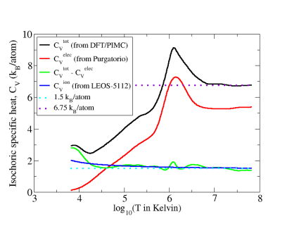
Figure 3: $C_{V}$ for CH at a density of $\rho=3.15$ g/cm³. The black curve is $C_{V}$ as extracted from a spline fit of our discrete $E(T)$ predictions from first-principles simulations at this density. See the text for descriptions of the other curves.

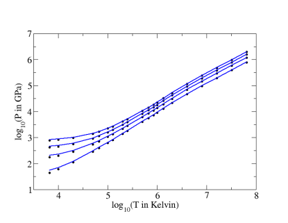
Figure 4: Total pressure isochores for CH at densities $\rho=$ 2.1, 3.15, 4.2, and 5.25 g/cm³ (in the sequence of bottom to top). The black symbols are the results of our DFT-MD ($T\leq 10^{6}$ K) and PIMC ($T>10^{6}$ K) simulations. The blue curves are the corresponding pressure isochores from LEOS-5112.

The terms in the free energy accounting for ionic excitations (ion-thermal) were modeled using both a Debye-Grüneisen model and a dissociation model. The Debye model used a Debye temperature of 650 K at equilibrium density and an ion-thermal Grüneisen $\gamma$ at this point of 0.99. This value of $\gamma$ was originally chosen to give the experimentally observed thermal expansion of GDP between 20 K and room temperature. The Grüneisen parameter was kept constant from $\rho_{0}$ up to a density of 2.7 g/cm³, at which point it was gradually decreased to 0.81 at 10 g/cm³ and 0.5 at very high density. For densities below 1.049 g/cm³, the Grüeneisen gamma reduces gradually to the ideal-gas value of 2/3. The variation in the Debye temperature is computed from this $\gamma(\rho)$ function More et al. (1988). The dissociation model adds an additional contribution to the free energy which models the dissociation of a dimer Young and Corey (1995). The main purpose of this term is to model chemical dissociation in a simplified way, as if it were due to diatomic molecular dissociation. In the GDP model, this extra flexibility allowed simultaneous fits to both Hugoniot data and off-Hugoniot release data. This same model was retained in LEOS-5112 without modification. The model includes a dimer dissociation energy of 0.7 eV and a nominal rotational temperature of 20 K.

The liquid contribution to the ion-thermal free energy in LEOS-5112 (and LEOS-5400) is given by a Cowan model More et al. (1988) with an exponent of 1/3,

$$C_{V}^{\rm ion}=\frac{3k_{B}}{2}+\frac{3k_{B}}{2}\left[\frac{T_{m}(\rho)}{T}\right]^{1/3}$$ (1)

This ensures that the ionic contribution to the specific heat decays from $3k_{B}/$ion to the ideal gas value of 1.5 $k_{B}/$ion as $T\rightarrow\infty$. $T_{m}(\rho)$ is taken to be the melt temperature, determined from the Lindemann relation More et al. (1988). Since CH dissociates before melting, it is necessary to assume a value for the melt temperature at ambient pressure. The value used here, $T_{m}$=513.15 K, is the same as that used in LEOS-5400 for GDP.

The electronic excitation contribution to the free energy of LEOS-5112 comes from the Purgatorio atom-in-jellium calculations Wilson et al. (2006) for carbon and hydrogen. The Purgatorio cold curve is replaced by a Thomas-Fermi cold curve, and some data adjustment is done in the low temperature region around equilibrium density to guarantee monotonicity in the pressure. These tables are then mixed using a constant-pressure, constant-temperature additive volume mix procedure. The resulting cold curve is then subtracted to yield the electron-thermal contribution used in the EOS. This includes the effects of shell structure, as well as relativistic effects at very high temperatures.

Figure 3 shows the specific heat at constant volume, $C_{V}$, for CH at a density of 3.15 g/cm³. The black curve is the result of calculating $(\partial E/\partial T)_{V}$ directly from the DFT-MD (for $T\leq 10^{6}$ K) and PIMC (for $T>10^{6}$ K) internal energies, by fitting a cubic spline to our 20 $E(T)$ points at this density and differentiating the smooth spline function. At the highest $T$, this asymptotes to 6.75 $k_{B}$/atom, which is the required value from equipartition, assuming complete ionization. There is a notable peak in this curve just above $10^{6}$ K. The red curve shows $C_{V}^{\rm electron}$ from LEOS-5112, obtained as described above from the Kohn-Sham DFT average-atom Purgatorio model Wilson et al. (2006). Though the peak is in a slightly different position than that seen in the black curve, this suggests that (a) the peak in $C_{V}$ at $T=10^{6}$ K arises from electronic ionization, and (b) this feature is modeled well by the comparatively simple Pugatorio treatment (which neglects, e.g., directional bonding). The temperature interval of the peak and related information presented in Refs. Zhang et al., 2017b; Hu et al., 2016a suggest that its appearance results primarily from the ionization of the 1s electron shell of carbon. The green curve shows the black curve minus the red curve, which is an estimation of the ionic contribution to $C_{V}$, assuming the perfect additivity of electronic and ionic components together with the use of Purgatorio for the electronic piece. Note that it approaches the required value of 1.5 $k_{B}$/atom at high-$T$ while rising slowly as $T$ decreases, ultimately rising rapidly to a value of $\sim 3k_{B}$/atom at the lowest $T$ (a value of $\sim$2.9 $k_{B}$/atom was predicted for CH_1.36 in Ref. Hamel et al., 2012). This rapid rise is reminiscent of behavior seen in DFT-MD calculations of pure carbon (see Fig. 9 of Ref. Benedict et al., 2014) where $C_{V}$ was shown to drop quickly from $3k_{B}$/atom with increasing $T$ over the range 2$\times 10^{4}$-8$\times 10^{4}$ K. Above a few times $10^{4}$ K, the general behavior of the green curve is tracked rather well by the blue curve, which shows $C_{V}^{\rm ion}$ from LEOS-5112 at this density, given by the form in Eq. 1. With the exception of the small discrepancies at the lowest $T$ of Fig. 3, the general agreement shown here provides validation for the manner in which the specific heat is modeled in LEOS-5112, indicating that at least the $T$-dependent part of $E$ is treated reasonably well. This is noteworthy, for the work on pure carbon Benedict et al. (2014) demonstrated that the model of Eq. 1 was suspect even for $T$ as high as $10^{6}$ K. The behavior shown in Fig. 3 is reproduced in our other energy isochores as well.

We further study the density dependence of $C_{V}(T)$ using LEOS 5112 in order to better understand the ionization process of CH. In Fig. 5, we show a comparison of the $C_{V}$ profiles over a much wider density range from $10^{-5}$-100 g/cm³ than we can access with existing simulation methods. For densities $\lesssim$0.1 g/cm³, we find two peaks: a narrow one above $3\times 10^{5}$ K corresponding to the ionization of the K shell (1s state), and a wide one at 10⁵ K due to the L shell of the carbon atoms. As the density increases, both peaks widen and shift to higher temperatures. These changes are due to the complex interplay of three effects: variations in the orbital shapes and an increase in size relative to the interatomic distances, a depletion of the 1s Fermi occupancy due to the temperature increase, and changes in the 1s binding energy due to variations in the screening effects. The K-shell peak in the heat capacity is predicted to disappear at $\sim$100 g/cm³, even though the 1s orbital is still bound at this density, and is not fully pressure ionized until a density of over 500 g/cm³. The suppression of the peak is a result of changes in the 1s binding energy as the 1s state is thermally depopulated. As the Fermi function reduces the occupancy of the orbital with increasing temperature, the binding energy of the 1s state increases due to a reduction in screening. This, in turn, raises the temperature required to depopulate the state, which results in a broadening of the heat capacity peak, leading to its apparent disappearance for the 100 g/cm³ case. This reduction-in-screening effect is present at all densities, but it is only at high enough densities since the heat capacity peak is shifted to sufficiently high temperatures so that it becomes undetectable when broadened. For densities less than 0.01 g/cm³, we also identified a shoulder in the L-shell peak at approximately 3$\times 10^{4}$ K, which we attribute to ionization effects of the hydrogen atoms because this shoulder is absent from the high-density carbon Purgatorio-based table.

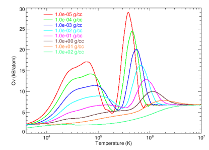
Figure 5: $C_{V}(T)$ of CH from LEOS 5112 at $10^{-5},10^{-4},10^{-3},10^{-2}$, 0.1, 1, 10, and 100 g/cm³.

While the temperature dependence of the internal energy of LEOS-5112 is therefore in quite good accord with that of our first-principles results throughout a wide range of density and temperature, the pressure of this model shows more significant discrepancies. Figure 4 shows isochores of $P$ for four densities, $\rho=$ 2.1, 3.15, 4.2, and 5.25 g/cm³. At the lower-$T$, the pressures of the model are systematically too high; near-perfect agreement is only seen at much higher temperature, approaching the ideal gas limit. This suggests that the Grüneisen $\gamma$ is too large in LEOS-5112, since this quantity does not enter the $C_{V}$ discussed above. Still another possibility is that the cold curve of LEOS-5112 can benefit from slight modification, though our current inclination is to reinvestigate the combined Debye-Grüneisen and dissociation models pertaining to the ionic excitation contribution. Work to improve the EOS models of hydrocarbons such as CH using these first-principles simulations is ongoing. In the following Sec. III.3, LEOS-5112 and LEOS-5400 are discussed again, in the context of predicted Hugoniot curves.

III.3 Shock compression

The locus of final states characterized by ($E,P,V$) accessible via a planar one-dimensional shock satisfy the Rankine-Hugoniot energy equation Mey

$$\mathcal{H}(T,\rho)=(E-E_{0})+\frac{1}{2}(P+P_{0})(V-V_{0})=0,$$ (2)

where ($E_{0},P_{0},V_{0}$) are the variables characterizing the initial (pre-shocked) state. This allows for the determination of the $P$-$V$-$T$ Hugoniot curve with bi-variable spline fitting of the EOS data ($E$ and $P$ on a grid of $T$ and $V$) in Sec. III.1.

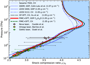
Figure 6: Comparison of the shock Hugoniot curve of CH and GDP from first-principles calculations (PIMC and DFT-MD simulations or linear-mixing approximation in this work, OF-DFT and DFT-MD simulations in Ref. Hu et al., 2015), EOS models (SESAME 7593 Lyon and Johnson (1992), QSEM Colin-Lalu et al. (2016), LEOS 5400 Sterne et al. (2016), LEOS 5112), and experiments Cauble et al. (1997, 1998); Ozaki et al. (2009); Barrios et al. (2010). Black circles are conditions chosen for examining the linear mixing approximation (see Sec. IV.1).

We thus obtain the principal Hugoniot curves of hydrocarbons Zhang et al. (2017b) and represent that of CH (assuming $\rho_{0}=1.05$ g/cm³ and $T_{0}=300$ K) in a pressure-density plot (Fig. 6) together with experimental measurements at low pressures Cauble et al. (1997, 1998); Ozaki et al. (2009); Barrios et al. (2010), OF-DFT simulations Hu et al. (2015), and the Purgatorio-based LEOS 5112 (described above), QSEM Colin-Lalu et al. (2016), and the SESAME 7593 Lyon and Johnson (1992) models. The DFT-MD predictions of the Hugoniot curve in this work and that of Ref. Hu et al., 2015 agree well with experimental measurements, whereas SESAME 7593 deviates from the experimental data at 1-4 TPa. At 0.5 Gbar, we predict CH to reach a maximum compression ($\rho/\rho_{0}$) of 4.7, which is similar to that predicted by the LEOS 5400 model for GDP, and is higher than that of QSEM Colin-Lalu et al. (2016), LEOS 5112, and OF-DFT Hu et al. (2015) by 2-5%; the SESAME 7593 model predicts the maximum compression to be smaller by 7.3% and the corresponding pressure about 17 megabar (Mbar) lower than our first-principles simulations. The compression maximum is originated from the 1s shell ionization of carbon. Since such temperature and pressure conditions correspond to the region at which PIMC works well and complexities such as electronic quantum effects, electronic correlation, and partial ionization are all essentially included in the quantum many-body framework, we expect the predictions in this work to be more reliable than those of semi-empirical models and OF-DFT. We note that the shock Hugoniot curve of CH obtained in this work is in remarkable agreement with that using a recent extended DFT method Zhang et al. (2016c); 201703communication (201). We look forward to accurate experiments in the Gbar regime which test these predictions.

Interestingly, our calculations and several other methods and models (Fig. 6) all have a shoulder along the Hugoniot curve at 4-fold compression. This corresponds to a pressure of 10 TPa and temperature of 5.7$\times 10^{5}$ K, according to the shock compression analysis of the first-principles EOS data in this work. The origin of this shoulder may be traced back to the start of ionization in the carbon 1s shell. Increasing amounts of carbon 1s electrons are excited at higher temperatures, as is shown in the $N(r)$ plot of Fig. 7. At $10^{6}$ K, a noticeable amount of excitation can be seen. The ionization fraction of the carbon 1s shell grows considerably as temperature increases even further. Above 8$\times 10^{6}$ K, 1s ionization is nearly complete and the system approaches an ideal plasma. Therefore the Hugoniot curves from different methods and models merge together and reach the ideal Fermi gas limit, which is consistent with the EOS comparisons and discussions in Sec. III.1.

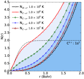
Figure 7: The average number of electrons $N(r)$ around each carbon or hydrogen nucleus in CH at 3.15 g/cm³ and a series of temperatures obtained from the PIMC simulations in this work. $N(r)$ is calculated via $N(r)=\left<\sum_{e,I}\theta(r-\left|\vec{r}_{e}-\vec{r}_{I}\right|)\right>/{N_{I}}$, where the sum includes all electron-carbon ion or electron-hydrogen ion pairs and $\theta$ represents the Heaviside function. The corresponding profile of the C⁴⁺ ionization state, calculated with GAMESS, is shown for comparison.

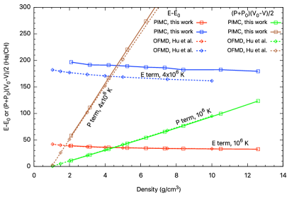
Figure 8: Comparison of the energy and pressure components of the Hugoniot function of CH from this work (solid lines and squares) and from the OF-DFT model Hu et al. (2015), dashed lines and diamonds) at two different temperatures. The initial state correspond to the ambient density of 1.05 g/cm³. The densities at which the energy and pressure terms agree solve Eq. 2 and may be realized in experiments.

In order to better understand the differences between the Hugoniot curves from our simulations and the OF-DFT and DFT-MD study in Ref. Hu et al., 2015, we compare the two components of the Hugoniot function in Fig. 8, i.e., the internal energy term $E-E_{0}$ and the pressure term $(P+P_{0})(V-V_{0})/2$, at two different temperatures. At $10^{6}$ K, data in this work and those of Ref. Hu et al., 2015 both rely on DFT-MD simulations, thus the energy and pressure values are similar. At $4\times 10^{6}$ K, the OF-DFT pressure is slightly lower than that given by PIMC and the difference between them grows larger for higher densities, whereas the internal energy from OF-DFT is significantly lower than that of PIMC, resulting in lower densities along the Hugoniot curve. The differences between the Hugoniot curves from the two methods are similar to those found for Si Hu et al. (2016a). These differences originate from the different treatments of electronic shell ionization effects in the two methods—PIMC is a many-body approach that accurately includes shell effects, while the OF-DFT approach makes use of what is essentially a Thomas-Fermi density functional which is not able to describe the shell structure accurately. Therefore, OF-DFT tends to smooth out ionization features near the compression maximum, leading to a single broad peak instead of the peak-shoulder (for CH) or double-peak (for Si) structures predicted by PIMC.

Note that zero-point motion has not been considered in our calculation of the reference energy $E_{0}$ nor in our DFT-MD simulations. To estimate its effect, we approximate Wal the harmonic zero-point energy with $\delta E=9k_{B}\Theta_{D}(V)/8$, where $k_{B}$ is the Bolzmann constant and $\Theta_{D}(V)$ is the volume-dependent Debye temperature, and the corresponding pressure $\delta P=9\gamma k_{B}\Theta_{D}(V)/8V$, where $\gamma$ is the Grüeneissen parameter, and add them to our DFT-MD EOS table of CH. $\Theta_{D}(V_{0})$ and $\gamma$ are approximated by 140 K and 1.2, respectively, by referring to the values of plastics in literature Amzel, Cucarella, and Becka (1971); Arp, Persichetti, and Chen (1984). With this zero-point correction, the compression ratio along the CH Hugoniot curve is reduced by a small amount of 0.01 for temperatures less than $10^{5}$ K. The maximum correction to our EOS occurs for the highest density of 12$\rho_{0}$, at which $\Theta_{D}(V)$ reaches a high value of 2761.5 K. However, the zero-point motion has a negligible effect ($<$0.3%) when comparing the EOS from PIMC and DFT-MD at 10⁶ K.

IV Discussion

IV.1 Structure of the hydrocarbon fluid

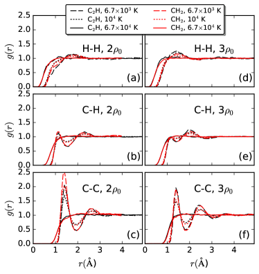
Figure 9: Comparison of the nuclear pair correlation function obtained from DFT-MD for C₂H (dark) and CH₂ (red) at two different densities for every material and three temperatures. The reference density $\rho_{0}$ is 1.76 and 2.24 g/cm³ for C₂H and CH₂, respectively.

In Ref. Zhang et al., 2017b, we have shown that the isothermal isobaric linear mixing approximation is very reasonable for hydrocarbons under stellar-core conditions. The validity of this approximation can be understood from analysis of the nuclear pair correlation functions, as is shown with the high-temperature (6.7$\times 10^{4}$ K) $g(r)$ profiles in Fig. S2 of Ref. Zhang et al., 2017b for CH and Fig. 9 for C₂H and CH₂. At these extreme conditions, no C-H bonds exist (lifetime shorter than 4.4 fs, see Table 1), and the non-existence of any peak structure in the pair-correlation function indicates that the system behaves similarly to an ideal yet partially ionized plasma. This explains the efficacy of the ideal linear mixing assumption manifested in the similarity between the Hugoniot curve as calculated from this approximation (using PIMC and DFT-MD EOS for the pure elements Hu et al. (2011); Benedict et al. (2014)), and the Hugoniot curve as calculated from our direct first-principles simulations of the mixtures in question Zhang et al. (2017b).

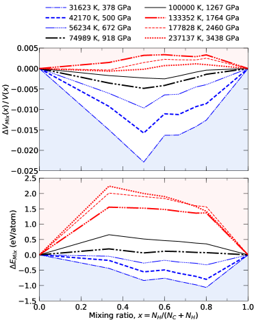
Figure 10: The difference in energy (top) and volume (bottom) between bi-variable spline fitting of our first-principles EOS data of CH and the linear mixing approximation at a series of $T,P$ conditions along the Hugoniot curve. The symbols are defined as $\Delta E_{Mix}(x)=E(x)-(1-x)E_{\text{C}}-xE_{\text{H}}$ and $\Delta V_{Mix}(x)=V(x)-(1-x)V_{\text{C}}-xV_{\text{H}}$.

Figure 10 compares the EOS of CH from interpolation of our first-principles data and that determined by the linear mixing approximation at a series of $T,P$ conditions along the Hugoniot curve (Fig. 6). In comparison to interpolation of our first-principles EOS data, linear mixing of pure C and pure H overestimates the volume of CH by 2.3% at 3.2$\times 10^{4}$ K (378 GPa). The volume difference $\Delta V_{mix}$ decreases to within $\pm$0.5% at $T>5.6\times 10^{4}$ K, which is consistent with the threshold temperature above which we see disappearance of peaks in the nuclear-pair correlation function $g(r)$ plots (Fig. 9). On the other hand, the energy of the linear mixture is higher than the first-principles value by 1.1 eV/atom at 3.2$\times 10^{4}$ K. The value of $\Delta E_{mix}$ decreases to 0-0.2 eV/atom at 7.5$\times 10^{4}$ K, and remains less than 2.5 eV/atom at higher temperatures. The fact that the energy of the linear mixture is smaller at the highest temperatures, while pressure is similar, explains why linear mixing predicts CH to be stiffer at the compression maximum than our direct first-principles predictions (Fig. 3 in Ref. Zhang et al., 2017b).

At lower pressure and temperature, clear signatures of chemical bonds exist. Figure 9 compares the $g(r)$ profile of C₂H and CH₂ at two different densities (2$\times$$\rho_{0}$ and 3$\times$$\rho_{0}$, with $\rho_{0}$= 1.76 and 2.24 g/cm³ for C₂H and CH₂, respectively) and three different temperatures. For C-C $g(r)$ functions in Fig. 9(c) and (f), the results show clear peaks and structure at both temperatures of 6.7$\times 10^{3}$ and $10^{4}$ K. These indicate the formation of carbon clusters. C-H bonds (Fig. 9(b) and (e)) also exist at these temperatures, characterized by the peak in $g(r)$ at $r$$\approx$1.15 Å. The C-H bonds are not very stable and are significantly weakened by thermal and compressional effects, as the differences in peak height show. We do not see any evidence of stable H-H bonds even at the the lowest temperature ($6.7\times 10^{3}$ K) that we considered (Fig. 9(a) and (d)), which is consistent with the analysis of other high pressure hydrogen-rich materials Vorberger et al. (2007); Soubiran and Militzer (2015). Interestingly, Ref. Sun et al., 2014 reported the formation of H₂ molecules during the dissociation of silane at low densities and temperatures of 1000-4000 K. Considerable amount of H₂ molecules were also found in H₂-H₂O mixtures at pressures below 35 GPa and a temperature of 2000 K Soubiran and Militzer (2015). Those conditions are much colder than we have considered in this study. In our simulations, the lifetime of H-H bonds is generally very short ($<$ 5 fs, see the following discussion and Table 1), which indicates no stable H₂ molecule can be formed. The peaks in $g(r)$ do not seem to be strongly dependent on the overall C:H ratio in the system and are consistent with findings in recent DFT-MD simulations Sherman et al. (2012) of CH₄.

A snapshot from the DFT-MD simulations of CH and its electronic density distribution at 3.15 g/cm³ and $2\times 10^{4}$ K is shown in Fig. 11. The disorder in the atomic positions is indicative of the plasma behavior, wherein ions participate in short-lived chemical bonding. Detailed structural analysis of the atomic bonding and lifetime  at this condition (see Table 1) indicates that C-C clusters and chains exist stably for the time scale of 10-100 fs, approximately one order of magnitude longer than H-H bonds. The lifetime of C-H bonds is slightly longer than 10 fs at $T<10^{4}$ K and $\rho<3.15$ g/cm³, and is shorter than 10 fs and about twice the value of H-H bonds at $T>10^{4}$ K.

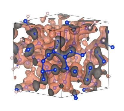
Figure 11: A snapshot of the electron density profile of CH in the polymeric state Sherman et al. (2012) around thermodynamic equilibrium at 3.15 g/cm³ and 2$\times 10^{4}$ K. The C and H atoms are represented by blue and pink spheres, respectively. Electron density which mitigates the bonding effects is illustrated by the light brown isosurface.

Table 1: Comparison of chemical bond lifetime $\tau$ in fs.

$\rho$ (g/cm3)	$T$ (K)	$P$ (Mbar)	$\tau_{\text{C-C}}$	$\tau_{\text{C-H}}$	$\tau_{\text{H-H}}$	$\tau_{\text{C-C-C}}$
2.10	6.7$\times 10^{3}$	0.44	89.62	16.68	4.60	44.12
2.10	1.0$\times 10^{4}$	0.61	48.77	11.36	4.00	23.92
3.15	6.7$\times 10^{3}$	1.76	69.72	12.63	4.18	35.67
3.15	1.0$\times 10^{4}$	2.04	43.13	10.19	3.80	21.72
3.15	2.0$\times 10^{4}$	2.89	25.63	7.58	3.15	12.93
3.15	5.0$\times 10^{4}$	5.55	14.63	5.06	2.28	7.55
3.15	6.7$\times 10^{4}$	7.19	12.44	4.34	2.06	6.58
3.15	1.3$\times 10^{5}$	13.4	9.50	3.30	1.60	4.88
3.15	2.0$\times 10^{5}$	22.1	7.47	2.68	1.32	3.85
3.15	5.1$\times 10^{5}$	60.9	4.70	1.66	0.88	2.47

Changes in chemical bonding in hydrocarbons have been proposed to interpret experimental results along the Hugoniot curves. For example, Barrios et al. Barrios et al. (2010) tentatively attributed a slight softening that is observed for polystyrene at 2-4 Mbar to the decomposition of chemical bonds. Bond dissociation is also included in the SESAME EOS model for CH at 2-4 Mbar Lyon and Johnson (1992). Our findings of dramatic decrease in the lifetimes of C-H bonds and changes in $g(r)$ at 0.4-4 Mbar are consistent with previous calculations Wang, He, and Zhang (2011); Hamel et al. (2012); Huser et al. (2015); Hu et al. (2015). However, our analysis shows that the decrease in bond lifetime is gradual, spaning a few Mbar and tens of thousands of Kelvin. This indicates that the dissociation of chemical bonds is continuous along the Hugoniot curve, instead of suddenly complete at certain $T$ and $P$.

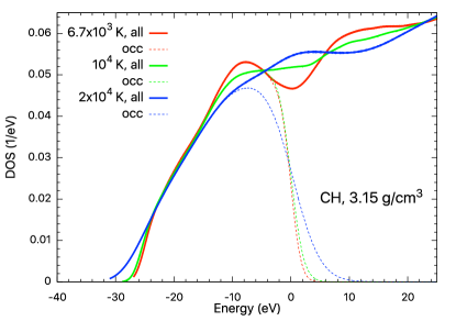
Figure 12: Electronic density of states (DOS) of CH at a series of temperatures and 3.15 g/cm³ based on DFT simulations. The dashed curves denote the occupied states. The Fermi energies are aligned at E=0 eV. A pseudo-bandgap exists at 6.7$\times 10^{3}$ K. With increasing temperature, the gap is gradually filled. We have compared the results by using the $\Gamma$ point, and 2$\times$2$\times$2 and 4$\times$4$\times$4 Monkhorst-Pack $k$ meshes Monkhorst and Pack (1976), and found very similar relationships between the three DOS curves.

We also investigated the electronic density of states of CH at the same ($\rho,T$) conditions as in the $g(r)$ analyses (Fig. 9). We find a pseudo-bandgap exists at the valence band maximum at 6.7$\times 10^{3}$ K. This gap is partially filled, resulting in a more continuous transition between the valence and the conduction bands, at $10^{4}$ K, and is completely filled at 2$\times 10^{4}$ K (see Fig. 12). Closure of the gap indicates metalization of the system, which increases the electrical conductivity and reflectivity that can be observed in experiments. The corresponding pressure range (1.5-2.5 Mbar) is in accord with experimental findings Barrios et al. (2010); Koenig et al. (2003) of optical reflectivity changes of CH samples. Note that band gap closure does not necessarily accompany complete chemical decomposition, because the changes in the lifetimes of the chemical bonds are gradual. It is therefore not appropriate to equate the origin of reflectivity change with chemical bond dissociation. We also do not see the changes in bonding to have an obvious effect on the shape of the Hugoniot curve.

IV.2 Composition dependence of the Hugoniot curve of GDP

ICF experiments routinely use GDP as an ablator material; GDP is mostly hydrocarbon (CH_1.36) doped with small amounts of heavier elements, such as O or Ge. As has been shown in Sec. IV.1 and in Ref. Zhang et al., 2017b, the linear mixing approximation is a reasonable way of estimating the EOS and shock compression of hydrocarbons. In this section, we apply this approximation to study the shock compression of GDP, compare with other EOS models, and investigate the effects of varying hydrogen and oxygen concentrations on the shock Hugoniot curve.

Figure 6 shows the Hugoniot curve of GDP (C₄₃H₅₆O), in comparison with those given by other models and that of CH. The initial density of GDP is set to 1.05 g/cm³, as relevant to polystyrene and to the hydrocarbon materials used in recent laser shock experiments Barrios et al. (2012). The initial energy $E_{0}$ is determined by approximating GDP as an ideal mixture of three polymers—PAMS (C₉H₁₀), polyethylene (C₂H₄) and polyvinylalcohol (C₂H₄O)—which allows for a higher flexibility in the composition of GDP. The energy of each polymer is determined as described in the supplementary material of Ref. Zhang et al., 2017b. We determine the energy of diamond, isolated H₂ and O₂ molecules using DFT calculations and combine them with tabulated thermochemical data on the enthalpy of combustion Roberts and Jessup (1951); Walters, Hackett, and Lyon (2000) to estimate the energy of these polymers. As a proof of concept, we compare the energy of coronene C₂₄H₁₂ determined as a combination of PAMS and polyethylene to the thermochemical data and find very small difference (less than 15 mHa/carbon). Initial densities in Fig. 13 are determined in the ideal mixture approximation, using the density of PAMS (1.075 g/cm³), polyethylene (0.95 g/cm³) and polyvinylalcohol (1.19 g/cm³).

Figure 6 shows the Hugoniot curve of GDP obtained from our first-principles EOS. It is slightly stiffer than that of CH at low pressures ($P<5$ Mbar) and near the compression maximum. Similar trends are found in the results of the QSEM model Colin-Lalu et al. (2016). For compression ratios between 3.3-4.3, a shoulder develops along the Hugoniot curve. The shoulder structure is also found along the Hugoniot curve of LEOS 5400 GDP, which exhibits higher compressibility than that predicted by the first-principles calculations in this work. This may be traced to the start of ionization of the 1s electron shell of carbon, which leads to the shoulder, and the much lower Grüeneisen $\gamma$ used in LEOS 5400 than in LEOS 5112 for compression ratios larger than 3.5, which causes the softer behavior predicted by LEOS 5400.

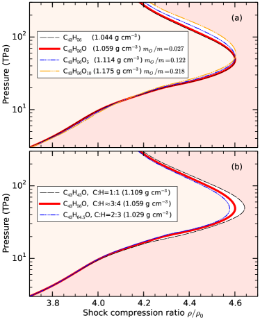
Figure 13: Comparison of the effects of varying oxygen (a) and hydrogen (b) content on the shock Hugoniot curve of GDP.

Considering that the chemical composition of GDP ablators varies Barrios et al. (2012); Colin-Lalu et al. (2016); Hamel et al. (2012); Sterne et al. (2016), it is thus useful to compare the Hugoniot curves of GDP with different C:H ratios and oxygen contents. We consider three oxygen mass percentages of 2.7%, 12.2%, and 21.8%, and C:H ratios of 1:1, 1:1.33, and 1:1.5. A comparison of the Hugoniot curves is shown in Fig. 13. With the addition of oxygen, the pressure at the maximum compression increases, while the compression ratio does not show any observable change. The effect of oxygen can be understood from the fact that its 1s electrons are more strongly bound to the oxygen nuclei, which requires a higher temperature for ionization. Changes to the maximum compression ratio are insignificant within the range of oxygen content that we consider, because the carbon 1s electrons dominate over those of oxygen. Increasing the amount of hydrogen leads to a decrease by 0.1 in the compression maximum when the C:H ratio decreases from 1:1 to 1:1.5, as shown in Fig. 13(b). This is the same trend with composition that has been seen in Fig. 3 of Ref. Zhang et al., 2017b. The pressure at the compression maximum is not affected.

V Conclusions

In this work, we presented the results of PIMC and DFT-MD simulations of a series of hydrocarbons. We obtained accurate internal energies and pressures from temperatures of 6.7$\times 10^{3}$ K to 1.3$\times 10^{8}$ K. PIMC and DFT-MD were shown to be consistent at $10^{6}$ K, typically to within 1 Ha/carbon in energy and 3% in pressure. This cross-validates the use of both methods at the temperature of $10^{6}$ K. We used these results to evaluate some of the detailed assumptions made in a recent EOS model for CH, LEOS-5112.

We investigated the principal Hugoniot curves using the obtained EOS data and found a maximum compression of 4.7, which is similar to that predicted by LEOS 5112 and 5400 but larger than SESAME 7593 and OF-DFT predictions. We expect future experiments will test this prediction.

We demonstrated the validity of the linear mixing approximation in obtaining the EOS and shock Hugoniot curves of hydrocarbons. This can be explained by the unstable, short-lived C-H chemical bonds (lifetime $\tau<4.4$ fs) for temperatures greater than $6.7\times 10^{4}$ K. The nuclear-pair correlation function $g(r)$ of hydrocarbons resembles that of a simple atomic liquid at the higher temperatures we considered. At lower temperatures, $g(r)$ as well as bond lifetime analysis of hydrocarbon systems show the possible existence of stable C-C bonds with lifetimes of 10-100 fs, weak C-H bonds with lifetimes of 4-16 fs, and no signature of stable H-H bonds.

By applying the linear mixing approximation, we investigated the Hugoniot curves of GDP as a function of oxygen content and C:H ratios. We found that the compression maximum remains unchanged when varying the oxygen mass percentage between 0 and 21.8% while the pressure increases by about 0.1 Gbar. When the C:H ratio decreases from 1:1 to 1:1.5, the shock compression maximum decreases by 0.1 while the pressure, which is determined by the 1s ionization of carbon, does not change.

Our results provide a benchmark for future theoretical investigations of the EOS of hydrocarbons, and should be useful for informing on-going dynamic compression experiments aimed at reaching Gbar conditions.

VI Supplementary Material

See the supplementary material for the tables of EOS data of C₂H, CH, C₂H₃, CH₂, CH₃, and CH₄ considered in this study.