The Einstein-Vlasov system in spherical symmetry II: spherical perturbations of static solutions

Abstract

We reduce the equations governing the spherically symmetric perturbations of static spherically symmetric solutions of the Einstein-Vlasov system (with either massive or massless particles) to a single stratified wave equation $-\psi_{,tt}=H\psi$, with $H$ containing second derivatives in radius, and integrals over energy and angular momentum. We identify an inner product with respect to which $H$ is symmetric, and use the Ritz method to approximate the lowest eigenvalues of $H$ numerically. For two representative background solutions with massless particles we find a single unstable mode with a growth rate consistent with the universal one found by Akbarian and Choptuik in nonlinear numerical time evolutions.

I Introduction

I.1 The Einstein-Vlasov system

The Vlasov-Einstein system describes an ensemble of particles of identical rest mass, each of which follows a geodesic. The particles interact with each other only through the spacetime curvature generated by their collective stress-energy tensor, whereas particle collisions are neglected.

For massive particles, this is a good physical model of a stellar cluster. For either massive or massless particles, the Einstein-Vlasov system also serves as a well-behaved toy model of matter in general relativity. In particular, spherically symmetric solutions of the Einstein-Vlasov system with small data are known to exist globally in time for massive ReinRendall1992 and massless particles Dafermos2006 . Self-similar spherically symmetric solutions with massless particles have been analyzed in JMMGundlach2002 and RendallVelazquez2011 . The existence of spherically symmetric static solutions with massive particles was proved in ReinRendall2000 , and there is numerical evidence that at least some are stable within spherical symmetry AndreassonRein2006 . Spherically symmetric static solutions with massless particles were analysed and constructed numerically in paperI , and we investigate their linear perturbations here. See also AndreassonLRR2011 for a review and additional references.

I.2 Motivation for this paper

This is the second paper in a series motivated by Akbarian and Choptuik’s AkbarianChoptuik (from now on, AC) recent study of numerical time evolutions of the massless Einstein-Vlasov system in spherical symmetry. AC found two apparently contradictory results:

I) Taking several 1-parameter families of generic smooth initial data and fine-tuning the parameter to the threshold of black hole formation, AC found what is known as type-I critical collapse: in the fine-tuning limit the time evolution goes through an intermediate static solution. The lifetime $\Delta\tau$ of this static solution increases with fine-tuning to the collapse threshold as

$$\Delta\tau\simeq\sigma\ln|p-p_{*}|+{\rm const},$$ (1)

where $p$ is the parameter of the family, $p_{*}$ its value at the black-hole threshold, and $\tau$ is the proper time at the centre, in units of the total mass of the critical solution. (1) implies the existence of a single unstable mode growing as $\exp(\tau/\sigma)$. AC found that $\sigma$ was approximately universal (independent of the family), with value $\sigma\simeq 1.4\pm 0.1$, and that the metric of the intermediate static solution was also approximately universal (up to an overall length and mass scale). In particular, its compactness $\Gamma:=\max(2M/r)$ was in the range $\Gamma\simeq 0.80\pm 0.01$ and its central redshift $Z_{c}\geq 0$ was in the range $Z_{c}\simeq 2.45\pm 0.05$.

II) Conversely, constructing static solutions by ansatz, AC found that these covered much larger ranges of $\Gamma$ and $Z_{c}$, but that each one was at the threshold of collapse. That is, adding a small generic perturbation to the static initial data and evolving in time with their nonlinear code, they found that for one sign of the perturbation the perturbed static solution collapsed while for the other sign it dispersed. They found that $\sigma$ was in the narrow range $\sigma\simeq 1.43\pm 0.07$, compatible with the value above.

Result II suggests that in spherical symmetry with massless particles, the black hole-threshold coincides with the space of static solutions. If so, then each static solution would have precisely one unstable mode (with its sign deciding between collapse and dispersion), with all other modes either zero modes (moving to a neighbouring static solution) or purely oscillating.

One aspect of Result I, namely that the spacetime of the critical solution is universal, would imply that this universal solution has one unstable mode (as before), but that all its other modes (including those tangential to the black hole threshold) are decaying ones, so that the attracting manifold of the critical solution is precisely the black hole threshold. Indeed, this is the familiar picture of type-I critical collapse in other matter-Einstein systems. However, this is in apparent contradiction to Result II.

In the first paper in this series paperI (from now Paper I), we used a symmetry of the massless spherically symmetric Einstein-Vlasov system to reduce its number of independent variables from four to three. We then numerically constructed static solutions with compactness in the range $0.7\simeq\Gamma\leq 8/9$. Based on this, we conjectured that the apparent contradiction above is resolved by the critical solution seen in fine-tuning generic initial data being universal only to leading order, and that this leading order is selected by the way in which it is approached during the evolution of generic smooth initial data.

To make further progress, it seems essential to analyse the spectrum of linear perturbations directly. This is the programme of the current paper. In contrast to the static solutions investigated in Paper I, their perturbations do not simplify significantly for $m=0$, and hence all of our analysis, except for the numerical examples in Sec. IV.5, will be for $m\geq 0$.

I.3 Plan of the paper

In order to make the presentation self-contained and to establish notation, we review some material from Paper I in Sec. II. We begin in Sec. II.1 by presenting the equations of the time-dependent spherically symmetric Einstein-Vlasov system. We do this in a form in which the massless particle limit is regular and leads to a reduction of the number of independent variables. We discuss static solutions in Sec. II.2, and the massless limit, for both the time-dependent and static case, in Sec. II.3.

In Sec. III we then derive the spherical perturbation equations. In Sec. III.1 we perturb the Vlasov and Einstein equations about a static background, splitting the perturbation of the Vlasov distribution function $f$ into parts $\phi$ and $\psi$ that are even and odd, respectively under reversing time. In Sec. III.2 we change independent variables from momentum to energy, as we did for the background solutions. We quickly dispense with static perturbations in Sec. III.3, and in Sec. III.4 we reduce the perturbed Vlasov and Einstein equations to a single integral-differential equation $-\psi_{,tt}=H\psi$. In Sec. III.5 we dispense with the relatively trivial perturbations on regions of phase space where the background solution is vacuum. We state the massless limit in Sec. III.6.

In Sec. IV we attempt to find the spectrum of eigenvalues. In Sec. IV.1 we identify a positive definite inner product with respect to which $H$ is symmetric. In Sec. IV.2 we rewrite the Hamiltonian as $H=A^{\dagger}A-D^{\dagger}D$ where $D$ is bounded, giving us at least a lower bound on $H$. We then switch to an approximation method, the Ritz method, which we review in Sec. IV.3. In Sec. IV.4 we specify some properties of the function space ${\mathbb{V}}$ in which to look for perturbation modes, that is eigenfunctions of $H$. In Sec. IV.5 we pick two specific background solutions that we obtained numerically in Paper I and use the Ritz method numerically. We find values of $\sigma$ in agreement with AC.

Sec. V contains a summary and outlook. Throughout the paper, $a:=b$ defines $a$, and we use units such that $c=G=1$.

II Background equations

II.1 Field equations in spherical symmetry

We consider the Einstein-Vlasov system in spherical symmetry, with particles of mass $m\geq 0$. We write the metric as

$$ds^{2}=-\alpha^{2}(t,r)dt^{2}+a^{2}(t,r)dr^{2}+r^{2}(d\theta^{2}+\sin^{2}\theta d\varphi^{2}).$$ (2)

To fix the remaining gauge freedom we set $\alpha(t,\infty)=1$. The Einstein equations give the following equations for the first derivatives of the metric coefficients:

$$\frac{\alpha_{,r}}{\alpha} = \frac{a^{2}-1}{2r}+4\pi ra^{2}p,$$ (3)

$$\frac{a_{,r}}{a} = -\frac{a^{2}-1}{2r}+4\pi ra^{2}\rho,$$ (4)

$$\frac{a_{,t}}{a} = 4\pi ra^{2}j,$$ (5)

where $p$, $\rho$ and $j$ are the radial pressure, energy density and radial momentum density, measured by observers at constant $r$. The fourth Einstein equation, involving the tangential pressure $p_{T}$, is a combination of derivatives of these three, and is redundant modulo stress-energy conservation.

The Vlasov density describing collisionless matter in general relativity is defined on the mass shell $p^{\mu}p_{\mu}=-m^{2}$ of the cotangent bundle of spacetime, or $f(t,x^{i},p_{i})$ in coordinates. We define the square of particle angular momentum

$$F:=p_{\theta}^{2}+\sin^{2}\theta\,p_{\varphi}^{2}.$$ (6)

In spherical symmetry this is conserved, leaving to $f=f(t,r,p_{r},F)$. In order to obtain a reduction of the Einstein-Vlasov system in the limit $m=0$, we replace $p_{r}$ by the new independent variable

$$z:={p_{r}\over a\sqrt{F}}.$$ (7)

The Vlasov equation for $f(t,r,z,F)$ is

$$\frac{\partial f}{\partial t}+{\alpha z\over aZ}\frac{\partial f}{\partial r}+\left({\alpha\over r^{3}aZ}-{\alpha_{,r}Z\over a}-{za_{,t}\over a}\right)\frac{\partial f}{\partial z}=0,$$ (8)

where we have defined the shorthand

$$Z(r,z,F):=\sqrt{{m^{2}\over F}+z^{2}+{1\over r^{2}}}={\alpha p^{t}\over\sqrt{F}}.$$ (9)

The non-vanishing components of the stress-energy tensor are

$$p:=T_{r}{}^{r} = \frac{\pi}{r^{2}}{\cal J}f\,{z^{2}\over Z},$$ (10)

$$\rho:=-T_{t}{}^{t} = \frac{\pi}{r^{2}}{\cal J}f\,Z,$$ (11)

$$j:=T_{t}{}^{r} = -\frac{\pi}{r^{2}}{\alpha\over a}{\cal J}f\,z,$$ (12)

$$p_{T}:={T_{\theta}}^{\theta}={T_{\varphi}}^{\varphi} = \frac{\pi}{2r^{4}}{\cal J}f\,{1\over Z},$$ (13)

where we have introduced the integral operator (acting to the right)

$${\cal J}:=\int_{0}^{\infty}FdF\int_{-\infty}^{\infty}dz.$$ (14)

II.2 Static solutions

In the static metric

$$ds^{2}=-\alpha_{0}^{2}(r)dt^{2}+a_{0}^{2}(r)dr^{2}+r^{2}(d\theta^{2}+\sin^{2}\theta d\varphi^{2})$$ (15)

with Killing vector $\xi:=\partial_{t}$, the particle energy

$$E:=-\xi^{\mu}p_{\mu}=-p_{t}=\alpha_{0}\sqrt{F}Z$$ (16)

is conserved along particle trajectories. In order to obtain a reduction of the static Einstein-Vlasov system in the limit $m=0$, we replace $E$ by

$$Q(r,z,F):={E^{2}\over F}=\alpha_{0}^{2}Z^{2}.$$ (17)

Hence we have

$$z=\pm\alpha_{0}(r)\sqrt{Q-U},$$ (18)

where we have defined

$$U(r,F):=\alpha_{0}^{2}\left({m^{2}\over F}+{1\over r^{2}}\right).$$ (19)

The general static solution of the Vlasov equation, for simplicity with a single potential well, is then given by

$$f(r,z,F)=k(Q,F).$$ (20)

(If $U$ forms more than one potential well, $k$ could be different in each of them Schaeffer1999 .)

The static Einstein equations are

$${\alpha_{0}^{\prime}\over\alpha_{0}} = {a_{0}^{2}-1\over 2r}+{4\pi^{2}a_{0}^{2}\over r}{\cal I}{k}{v},$$ (21)

$${a_{0}^{\prime}\over a_{0}} = -{a_{0}^{2}-1\over 2r}-{4\pi^{2}a_{0}^{2}\over r}{\cal I}{{k}\over{v}},$$ (22)

where we have defined the integral operator (acting to the right)

$${\cal I}:=\int_{0}^{\infty}FdF\int_{{U(r,F)}}^{\infty}\,dQ$$ (23)

and the shorthand

$${v}(r,Q,F):={|z|\over Z}={a|p^{r}|\over\alpha p^{t}}.$$ (24)

From (17) and (9) we have $dQ=2\alpha_{0}^{2}z\,dz$, and hence on a static background, where ${\cal I}$ is defined, it is related to ${\cal J}$ by

$${\cal I}=\alpha_{0}^{2}{\cal J}z.$$ (25)

The second equality in (24) shows that $\pm v$ is the radial particle velocity, expressed in units of the speed of light and measured by static observers. (Note that by definition $v\geq 0$.) The fact that (24) can be rewritten as

$$v=\sqrt{1-{U\over Q}}$$ (26)

shows that $U$ is an effective potential for the radial motion of the particles with given constant “energy” $Q$ and angular momentum squared $F$. In particular $Q=U(r,F)$ determines the radial turning points $r$ for all particles with a given $Q$ and $F$.

We define $U_{0}(F)$ as the value of $U(r,F)$ at its one local maximum $r_{0+}(F)$ in $r$. We define $r_{0-}(F)$ as the other value of $r$ for which $U$ takes the same value. We also define $U_{3}(F)$ as the value of $U(r,F)$ at its one local minimum $r_{3}(F)$ in $r$. Intuitively, $U_{0}(F)$ is the “lip” of the effective potential for particles of a given $F$, and $U_{3}(F)$ its “bottom”. We define $U_{1}(F)\leq U_{0}(F)$ as the upper boundary in $Q$ of the support of $k(Q,F)$ and $U_{2}(F)\geq U_{3}(F)$ as the lower boundary. We define $r_{1\pm}(F)$ and $r_{2\pm}(F)$ as the values where $Q=U_{1}(F)$ or $Q=U_{2}(F)$.

For massless particles, particles with all values of $F$ move in the same potential $U=U(r)$, and all other quantities we have just defined do also not depend on $F$. See Fig. 1 for an illustration.

Any particles with $Q>U_{0}(F)$ would be unbound, and if such particles were present in a static solution with the ansatz (20) they would be present everywhere and hence the total mass could not be finite. We must therefore have $k(Q,F)=0$ for $Q>U_{0}(F)$. $k(Q,F)$ must either have compact support in $F$, or fall off as $F\to\infty$ sufficiently rapidly for $\int kFdF$ to be finite. Both assumptions are assumed implicitly in the definition (23) of ${\cal I}$ when we formally extend the upper integration limits in $Q$ and $F$ to $\infty$.

By contrast, real values of $z$ require $Q\geq U(r,F)$, and when changing from $\int dz$ to $\int dQ$, the condition $Q\geq U$ must be imposed explicitly as a limit to the integration range in (23). Hence $k(Q,F)$ needs to be defined for all $U_{3}(F)\leq Q\leq U_{0}(F)$ (it can be zero in part of that range), but not all of that range contributes to the integral ${\cal I}$, and hence to the stress-energy tensor, at every value of $r$.

II.3 Reduction of the field equations for $m=0$

Because $F$ is conserved, the field equations already do not contain $\partial/\partial F$. Furthermore, $m$ and $F$ appear in the coefficients of the field equations only in the combination $m^{2}/F$. In the limit $m=0$, these coefficients become independent of $F$. As first used in JMMGundlach2002 , the integrated Vlasov density

$$\bar{f}(t,r,z):=\int_{0}^{\infty}f(t,r,z,F)FdF$$ (27)

then obeys the same PDE (8) as $f$ itself. The stress-energy tensor is now given by the expressions (10-13) above, with $\bar{f}$ in place of $f$, and

$${\bar{\cal J}}:=\int_{-\infty}^{\infty}dz$$ (28)

in place of ${\cal J}$. We have reduced the Einstein-Vlasov system to a system of integral-differential equations in the independent variables $(t,r,z)$ only. A solution $(a,\alpha,\bar{f})$ of the reduced system represents a class of solutions $(a,\alpha,f)$, all with the same spacetime but different matter distributions.

Similarly, in the static case with $m=0$ the Einstein equations are given by (21-22) with

$$\bar{k}(Q):=\int_{0}^{\infty}{k}(Q,F)FdF$$ (29)

in place of $k(Q,F)$ and

$${\bar{\cal I}}:=\int_{{U(r)}}^{\infty}\,dQ$$ (30)

in place of ${\cal I}$. Each solution of the reduced system $(a_{0},\alpha_{0},\bar{k})$ represents a class of solutions $(a_{0},\alpha_{0},k)$. We now define $U_{1}$ and $U_{2}$ as the limits of support of $\bar{k}(Q)$.

In Paper I, we conjectured that the space of spherically symmetric static solutions with massless particles is a space of single functions of one variable, subject to certain positivity and integrability conditions. This single function can be taken to be any one of $\alpha_{0}(r)$, $a_{0}(r)$ or $\bar{k}(Q)$.

As a postscript to Paper I, we note here that a mathematically similar result holds for Vlasov-Poisson system for a subclass of static solutions, namely the “isotropic” ones, where the Vlasov function is assumed to be a function of energy only. With the isotropic ansatz the Vlasov density uniquely defines the Newtonian gravitational potential and vice versa DeJonghe . Physically, however, the two results are different, as the relativistic result with massless particles holds for all solutions, depending on both energy and angular momentum.

III Spherical perturbation equations

III.1 Perturbation ansatz

In the study of the linear perturbations of a static solution we return to the general case $m\geq 0$. We make the perturbation ansatz

$$\alpha(t,r) = \alpha_{0}(r)+\delta\alpha(t,r),$$ (31)

$$a(t,r) = a_{0}(r)+\delta a(t,r),$$ (32)

$$f(t,r,z,F) = {k}({Q},F)+\phi(t,r,z,F)$$ (33)

$$+\,\psi(t,r,z,F),$$

where $(\alpha_{0},a_{0},k)$ is a static solution of the Einstein-Vlasov system, and where $Q$ is given by (17). We define $\phi$ to be even in $z$ and $\psi$ to be odd. In particular, as $\delta f(t,r,z,F)$ must be at least once continuously differentiable ($C^{1}$) to obey the Vlasov equation in the strong sense, its odd-in-$z$ part must vanish at $z=0$, or

$$\psi(t,r,z=0,F)=0.$$ (34)

We now expand to linear order in the perturbations. The linearised Vlasov equation splits into the pair

$$\phi_{,t}+{L}\psi = 2Qk_{,Q}{{v}^{2}\over a_{0}}\delta a_{,t},$$ (35)

$$\psi_{,t}+{L}\phi = 2Qk_{,Q}{{v}\alpha_{0}\over a_{0}}\left({\delta\alpha\over\alpha_{0}}\right)_{,r},$$ (36)

where we have defined the differential operator

$${L}:={z\alpha_{0}\over Za_{0}}{\partial\over\partial r}+\left({\alpha_{0}\over a_{0}r^{3}Z}-{Z\alpha_{0}^{\prime}\over a_{0}}\right){\partial\over\partial z}.$$ (37)

Note, from (8), that the time-dependent Vlasov equation in the fixed static spacetime $(a_{0},\alpha_{0})$ is $f_{,t}+{L}f=0$. By construction, ${Q}$ obeys ${L}{Q}=0$, and hence ${L}{k}({Q},F)=0$, as we have already used to construct static solutions. The even-odd split of the perturbed Vlasov equation into the pair (35,36) reflects the fact that reversing both $t$ and $z$ together must leave the field equations invariant.

The perturbed Einstein equations are

$$\left({\delta\alpha\over\alpha_{0}}\right)_{,r}-\left({1\over r}+{2\alpha_{0}^{\prime}\over\alpha_{0}}\right){\delta a\over a_{0}} = {4\pi^{2}a_{0}^{2}\over r}{\cal J}{z^{2}\over Z}\phi,$$ (38)

$$\left({r\delta a\over a_{0}^{3}}\right)_{,r} = 4\pi^{2}{\cal J}Z\phi,$$ (39)

$$\delta a_{,t} = -{4\pi^{2}a_{0}^{2}\over r}{\cal J}z\psi.$$ (40)

We have used the background Einstein equations to eliminate all integrals of $k$ in favour of $a_{0}^{\prime}$ and $\alpha_{0}^{\prime}$. The integrability condition for $\delta a$ between (39) and (40) is identically obyed modulo the perturbed Vlasov equation (35,36), and hence the perturbed Einstein equation (40) is redundant [just as (5) is in the nonlinear equations].

III.2 Change of variable from $z$ to $Q$

To simplify the perturbation equations, we change independent variables from $(t,r,z,F)$ to $(t,r,Q,F)$, with $Q$ again given by (17). From the resulting transformation of partial derivatives, we need only the following identities:

$$\left.{\partial\over\partial t}\right|_{z} = \left.{\partial\over\partial t}\right|_{Q},$$ (41)

$$\left.{\partial\over\partial r}\right|_{z} = \left.{\partial\over\partial r}\right|_{Q}+(\dots)\left.{\partial\over\partial Q}\right|_{r},$$ (42)

$${L} = {V}\left.{\partial\over\partial r}\right|_{Q},$$ (43)

where we have defined the shorthand

$${V}(r,Q,F)={\alpha_{0}\over a_{0}}{v},$$ (44)

with $v$ given by (26). $V$ is the coordinate speed $dr/dt$ corresponding to the physical speed $v$.

$\partial/\partial r|_{z}$ on its own appears in the field equations only acting on the metric and its perturbations, in which case the $\partial/\partial Q|_{r}$ term denoted by $(\dots)$ in (42) is irrelevant. On the matter perturbations, $\partial/\partial r|_{z}$ acts only in the combination ${L}$. From now on $\partial/\partial r$ is understood to mean $\partial/\partial r|_{Q}$.

With (43) the perturbed Vlasov equation becomes

$$\phi_{,t}+V\psi_{,r} = 2Qk_{,Q}{{v}^{2}\over a_{0}}\delta a_{,t},$$ (45)

$$\psi_{,t}+V\phi_{,r} = 2Qk_{,Q}{{v}\alpha_{0}\over a_{0}}\left({\delta\alpha\over\alpha_{0}}\right)_{,r}.$$ (46)

With (25) and (24) the perturbed Einstein equations (38-40) become

$$\left({\delta\alpha\over\alpha_{0}}\right)_{,r}-\left({1\over r}+{2\alpha_{0}^{\prime}\over\alpha_{0}}\right){\delta a\over a_{0}} = {4\pi^{2}a_{0}^{2}\over r\alpha_{0}^{2}}{\cal I}{v}\phi,$$ (47)

$$\left({r\delta a\over a_{0}^{3}}\right)_{,r} = {4\pi^{2}\over\alpha_{0}^{2}}{\cal I}{\phi\over{v}},$$ (48)

$$\delta a_{,t} = -{4\pi^{2}a_{0}^{2}\over r\alpha_{0}}{\cal I}\psi.$$ (49)

Equivalently, the stress-energy perturbations are given by

$$\delta p = {\pi\over r^{2}\alpha_{0}^{2}}{\cal I}v\phi,$$ (50)

$$\delta\rho = {\pi\over r^{2}\alpha_{0}^{2}}{\cal I}{\phi\over v},$$ (51)

$$\delta j = -{\pi\over r^{2}\alpha_{0}a_{0}}{\cal I}\psi.$$ (52)

Finally, the boundary condition on $\psi$ becomes

$$\psi(t,r,U(r,F),F)=0.$$ (53)

III.3 Static perturbations

Static perturbations can be obtained more directly by linear perturbation of the nonlinear static equations. The infinitesimal change $k\to k+\delta k$, $a_{0}\to a_{0}+\delta a_{0}$, $\alpha_{0}\to\alpha_{0}+\delta\alpha_{0}$ to a neighbouring static solution gives

$$\phi = \left.{d\over d\epsilon}\right|_{\epsilon=0}(k+\epsilon\delta k)\left((\alpha_{0}+\epsilon\delta\alpha)^{2}Z^{2},F\right)$$ (54)

$$= \delta k(Q,F)+2Qk_{,Q}{\delta\alpha\over\alpha_{0}},$$

$$\psi = 0.$$ (55)

As expected, this solves the perturbed Vlasov equations (45-46) and Einstein equation (49) identically for arbitrary functions $\delta k(Q,F)$, modulo the nontrivial perturbed Einstein equations (47-48).

III.4 Reduction to a single stratified wave equation

We can uniquely split any time-dependent perturbation that admits a Fourier transform with respect to $t$ into a static part (with frequency $\omega=0$) and a genuinely non-static part (with frequencies $\omega\neq 0$). For genuinely non-static perturbations we can uniquely invert $\partial/\partial t$ by dividing by $i\omega$ in the Fourier domain.

We now substitute (49) into (45), and (47) and $\left({\partial\over\partial t}\right)^{-1}(\ref{deltaadotm})$ into (46), and write the result in the compact form

$$\left(\begin{array}[]{cc}{\partial\over\partial t}&A\\ B&{\partial\over\partial t}+\left({\partial\over\partial t}\right)^{-1}C\end{array}\right)\left(\begin{array}[]{cc}\phi\\ \psi\end{array}\right)=0,$$ (56)

where we have defined the integral-differential operators (acting to the right)

$$A := {L}+g{v}{\cal I},$$ (57)

$$B := {L}-g{\cal I}{v},$$ (58)

$$C := hg{\cal I}$$ (59)

with the differential operator ${L}$ now given by (43), the integral operator ${\cal I}$ defined in (23) (both acting to the right), $v$ given by (26), and the shorthand expressions

$$g(r,Q,F) := {8\pi^{2}a_{0}\over r\alpha_{0}}Q\,k_{,Q}\,{v},$$ (60)

$$h(r) := {\alpha_{0}\over a_{0}}\left({1\over r}+{2\alpha_{0}^{\prime}\over\alpha_{0}}\right).$$ (61)

Note that $A$, $B$, $C$ do not commute with each other, while $\partial/\partial t$ commutes with all of them because their coefficients are independent of $t$.

In this compact notation it is easy to see that by row operations we can reduce the system (56) to the upper diagonal form

$$\left(\begin{array}[]{cc}{\partial\over\partial t}&A\\ 0&\left({\partial\over\partial t}\right)^{2}+C-BA\end{array}\right)\left(\begin{array}[]{cc}\phi\\ \psi\end{array}\right)=0.$$ (62)

Hence we have reduced the time-dependent problem to the single integral-differential equation

$$-\psi_{,tt}=H\psi,$$ (63)

where

$$H:=C-BA=hg{\cal I}-({L}-g{\cal I}{v})({L}+g{v}{\cal I}).$$ (64)

The coefficients $g$, $h$, $v$ and $V$ commute with each other but not with the operators $\partial/\partial r$ or ${\cal I}$. $\partial/\partial r$ and ${\cal I}$ do commute with each other because of the boundary condition (53).

It is convenient to split the time evolution operator $H$ into a kinematic and a gravitational part as

$$H=H_{0}+H_{1},$$ (65)

with

$$H_{0} := -L^{2}=-V{\partial\over\partial r}V{\partial\over\partial r},$$ (66)

$$H_{1} := g\left(h+\left({\cal I}v^{2}g\right)\right){\cal I}+g{\cal I}v{L}-{L}gv{\cal I}$$

$$= \left[g\left(h+\left({\cal I}v^{2}g\right)\right)-(Lgv)\right]{\cal I}+g\left({\cal I}v{L}-v{L}{\cal I}\right).$$

Hence we can write (63) as

$$-\psi_{,tt}+V{\partial\over\partial r}V{\partial\over\partial r}\psi=H_{1}\psi.$$ (69)

This form stresses that (69) is a stratified wave equation, in the sense that for fixed $Q$ and $F$ we have a wave equation in $(t,r)$, with coefficients also depending on $Q$ and $F$, while different values of $Q$ and $F$ are also coupled through the double integral ${\cal I}$ over $Q$ and $F$, which represents the gravitational interactions between particles of different momenta at the same spacetime point. Intuitively, the characteristic speeds of (69) are $\pm{V}$ because any matter perturbation is propagated simply at the velocity of its constituent particles.

We note in passing that in our notation the static perturbations are solutions of

$$B\phi=0,\qquad\psi=0.$$ (70)

Given a solution $\psi$ of the master equation (63), $\phi$ in any genuinely nonstatic perturbation can be reconstructed from $\psi$ as

$$\phi=-\left({\partial\over\partial t}\right)^{-1}A\psi,$$ (71)

and the metric perturbations are obtained by solving (47-48), with (49) obeyed automatically.

III.5 Preliminary classification of non-static perturbations

The right-hand side of (69) is generated by perturbations at all values of $Q$ and $F$ at at given spacetime point $(t,r)$, but because of the overall factor $k_{,Q}$ it only acts on perturbations at those values of $Q$ and $F$ where $k_{,Q}(Q,F)\neq 0$, that is, where background matter is present.

This suggests a preliminary classification of all perturbations into

• stellar modes, with support on the region in $(r,Q,F)$ space that lies inside the potential well and where also $k(Q,F)$ has support;

• bottom modes, with support inside the potential well and for values of $Q$ below the support of $k(Q,F)$;

• middle modes, with support inside the potential well and for values of $Q$ above the support of $k(Q,F)$ but below the top of the potential well;

• outer modes, with support outside the potential well and for values of $Q$ below the top of the potential well;

• top modes, with values of $Q$ above the top of the potential well.

This classification of modes is illustrated in Fig. 1 for the massless case, where all values of $F$ experience the same effective potential $U(r)$. Obviously, the middle modes do not exist if the potential well is filled to the top ($U_{1}=U_{0}$), and the bottom modes do not exist if it is filled to the bottom ($U_{2}=U_{3}$).

Figure 1: Sketch of the potential $U(r)$ for massless particles, illustrating the classification of perturbations. The black hatching shows the region in $(U,r)$ space where particles are present in the background solution. Outer modes have support in the green region, top modes in the yellow region, middle modes in the red region, bottom modes in the blue region, and stellar modes in the hatched region only. (The top, middle and bottom modes also drive stellar modes.) This figure can also be interpreted as the cross-section $U(r,\infty)$ of the potential $U(r,F)$ in the massive case, compare the definition (19) of $U$.

Particles contributing to the bottom, middle, top and outer modes move freely in the effective potential $U(r,F)$ set by the static background solution, without experiencing a gravitational back-reaction. We may call them the trivial modes. Mathematically, the trivial modes obey (69) in a region of $(Q,F)$ space where the right-hand side vanishes. In that region they can be solved in closed form. To do this, we define the “tortoise radius”

$$\sigma(r,Q,F):=\int^{r}{1\over{V}(r^{\prime},Q,F)}\,dr^{\prime}.$$ (72)

This gives us

$$L={V}\left.{\partial\over\partial r}\right|_{Q}=\left.{\partial\over\partial\sigma}\right|_{Q},$$ (73)

and hence (69) becomes

$$-\psi_{,tt}+\psi_{,\sigma\sigma}=0$$ (74)

for $\psi(t,\sigma,Q,F)$, subject to the Dirichlet boundary conditions

$$\psi(t,\sigma_{-}(Q,F),Q,F)=\psi(t,\sigma_{+}(Q,F),Q,F)=0,$$ (75)

where $\sigma_{\pm}$ are the left and right turning points given by $Q=U$. Hence we can write down the general local solution of (69) with $S=0$ in d’Alembert form as

$$\psi(t,r,Q,F)=\sum_{\pm}\psi_{\pm}\left[t\pm\sigma(r,Q,F),Q,F\right]$$ (76)

subject to the boundary conditions (75).

With $g=0$ for the trivial modes, (71) becomes $\phi_{,t}+\psi_{,\sigma}=0$, and hence

$$\phi(t,r,Q,F)=\sum_{\pm}\mp\psi_{\pm}\left[t\pm\sigma(r,Q,F),Q,F\right].$$ (77)

We note also that $\psi+\phi$ must be non-negative for physical trivial modes, as we cannot subtract particles from a vacuum region.

The trivial modes (except for the outer modes) induce stellar modes through gravitational interactions, or mathematically through the right-hand side of (69). This means that for a complete solution of the problem, we need to solve for stellar modes including an arbitrary driving term generated by the other modes, that is

$$-\psi_{,tt}+V{\partial\over\partial r}V{\partial\over\partial r}\psi=H_{1}\psi+H_{1}\psi_{\rm ext}$$ (78)

where $\psi$ describes the stellar modes and $\psi_{\rm ext}$ is the sum of the top, middle and bottom modes. (The outer modes do not couple to the stellar modes at all.)

III.6 Massless case

In the massless case, we define the integrated matter perturbations in the obvious way:

$${\bar{\phi}}(t,r,Q) := \int_{0}^{\infty}\phi(t,r,Q,F)\,FdF,$$ (79)

$${\bar{\psi}}(t,r,Q) := \int_{0}^{\infty}\psi(t,r,Q,F)\,FdF.$$ (80)

The reduced perturbation equations with $m=0$ are obtained from the ones in the general case by replacing $\phi$ and $\psi$ with $\bar{\phi}$ and $\bar{\psi}$, $k(Q,F)$ and $k_{,Q}(Q,F)$ with $\bar{k}(Q)$ and $\bar{k}^{\prime}(Q)$, and ${\cal I}$ with ${\bar{\cal I}}$. The coefficients $g$, $v$, $V$ and $U$ all become independent of $F$. In particular, all particles now move in the same effective potential $U(r)$.

IV Perturbation spectrum

IV.1 Inner product

Starting from (III.4), we rewrite the gravitational part $H_{1}$ of the Hamiltonian more explicitly as

$$H_{1} = Xc_{1}{\cal I}+X\left(c_{2}{\cal I}v^{2}{\partial\over\partial r}-{\partial\over\partial r}c_{2}v^{2}{\cal I}\right).$$ (81)

where we have defined the shorthands

$$X(Q,F,r) := Qk_{,Q}V,$$ (82)

$$c_{0}(r) := {8\pi^{2}a_{0}^{2}\over r\alpha_{0}^{2}},$$ (83)

$$c_{1}(r) := {8\pi^{2}a_{0}\over r\alpha_{0}}\left({1\over r}+{2\alpha_{0}^{\prime}\over\alpha_{0}}+c_{3}\right),$$ (84)

$$c_{2}(r) := {8\pi^{2}a_{0}\over r\alpha_{0}},$$ (85)

$$c_{3}(r) := {8\pi^{2}a_{0}^{2}\over r\alpha_{0}^{2}}{\cal I}{v}^{3}\,Q\,k_{,Q}.$$ (86)

We have defined $c_{0}$ for later use: note that $g=c_{0}X$. For clarity we have not written out function arguments, but recall that ${\cal I}$ acting on anything gives a function of $t$ and $r$ only, that $k=k(Q,F)$, $v^{2}=1-U/Q$, $U=U(r,m^{2}/F)$, and hence that $v=v(r,Q,m^{2}/F)$ and $V=V(r,Q,m^{2}/F)$.

We now construct an inner product $\langle\psi_{1},\psi_{2}\rangle$ with respect to which $H$ is a symmetric operator. Consider first solutions $\psi_{1}$, $\psi_{2}$ with support only where $k_{,Q}(Q,F)=0$, that is the modes we have characterised as trivial. Then only $H_{0}\psi$ is non-vanishing, and the perturbed Vlasov equation reduces to the free wave equation (74). The obvious inner product is therefore the well-known one for the free wave equation, that is

$$\langle\psi_{1},\psi_{2}\rangle:=\int_{0}^{\infty}\!\!\!\!\int_{0}^{\infty}\!\!\left(\int_{\sigma_{-}(Q,F)}^{\sigma_{+}(Q,F)}\psi_{1}\psi_{2}\,d\sigma\right)\mu(Q,F)\,dQ\,FdF,$$ (87)

where $\mu(Q,F)>0$ is an arbitray weight. Expressing this in terms of $r$, we have

$$\langle\psi_{1},\psi_{2}\rangle=\int_{0}^{\infty}\!\!\!\!\int_{0}^{\infty}\!\!\!\left(\int_{r_{-}(Q,F)}^{r_{+}(Q,F)}{\psi_{1}\psi_{2}\,dr\over V(r,Q,F)}\right)\mu(Q,F)\,dQ\,FdF.$$ (88)

If we interchange the integration over $r$ with the double integration over $Q$ and $F$, we obtain

$$\langle\psi_{1},\psi_{2}\rangle = \int_{0}^{\infty}\!\!\!\!\int_{0}^{\infty}\!\!\!\left(\int_{U(r,F)}^{\infty}{\mu(Q,F)\psi_{1}\psi_{2}\,dQ\over V(r,Q,F)}\right)FdF\,dr$$ (89)

$$= \int_{0}^{\infty}\!\!\left({\cal I}{\mu\psi_{1}\psi_{2}\over V}\right)dr$$

Integration by parts in $r$ in (88), and then transforming to (89), then gives

$$\langle\psi_{1},H_{0}\psi_{2}\rangle=\int_{0}^{\infty}\!\!\!\left({\cal I}\mu V\psi_{1,r}\psi_{2,r}\right)\,dr=\langle V\psi_{1,r},V\psi_{2,r}\rangle,$$ (90)

which is explicitly symmetric in $\psi_{1}$ and $\psi_{2}$.

Consider now solutions $\psi_{1}$, $\psi_{2}$ with support only where $k_{,Q}(Q,F)\neq 0$, that is stellar modes. Assuming further that $k_{,Q}<0$ wherever $k\neq 0$ (as will be the case for our examples), we must then make the choice

$$\mu(Q,F)=-{1\over Qk_{,Q}}$$ (91)

(up to a positive constant factor), that is

$$\langle\psi_{1},\psi_{2}\rangle = -\int_{0}^{\infty}\!\!\!\left({\cal I}{\psi_{1}\psi_{2}\over X}\right)\,dr$$ (92)

$$= -\int_{0}^{\infty}\!\!\!\!\int_{0}^{\infty}\!\!\!\left(\int_{r_{-}}^{r_{+}}{\psi_{1}\psi_{2}\over X}\,dr\right)\,dQ\,FdF,$$ (93)

with $X$ defined in (82). We then find from (90), (92) and (81) that

$$\langle\psi_{1},H_{0}\psi_{2}\rangle = -\int_{0}^{\infty}\left({\cal I}{V^{2}\psi_{1,r}\psi_{2,r}\over X}\right)dr,$$ (94)

$$\langle\psi_{1},H_{1}\psi_{2}\rangle = -\int_{0}^{\infty}c_{1}({\cal I}\psi_{1})({\cal I}\psi_{2})\,dr$$ (95)

$$-\int_{0}^{\infty}c_{2}\bigl{[}({\cal I}\psi_{1})({\cal I}v^{2}\psi_{2,r})$$

$$\qquad+({\cal I}\psi_{2})({\cal I}v^{2}\psi_{1,r})\big{]}\,dr,$$

where for the last term we have used integration by parts in $r$.

We now define $\mu(Q,F)>0$ on all of phase space by (91) on the support of $k(Q,F)$, and an arbitrary positive $\mu$, for example $\mu=1$, everywhere else.

IV.2 Quadratic form of the Hamiltonian

Consider the operator

$$\qquad{P}:={X{\cal I}\over({\cal I}X)}.$$ (96)

It is easy to see that ${P}$ is a projection operator, in the sense that

$${P}^{2}={P}.$$ (97)

We also have

$$\langle\psi_{1},{P}\psi_{2}\rangle=\int dr\,{\cal I}{\psi_{1}\over X}{X({\cal I}\psi_{2})\over({\cal I}X)}=\int dr\,{({\cal I}\psi_{1})({\cal I}\psi_{2})\over({\cal I}X)},$$ (98)

and so ${P}$ is symmetric,

$${P}^{\dagger}={P}.$$ (99)

As a projection operator, ${P}$ can only have eigenvalues $0$ and $1$. The corresponding eigenspaces $\hat{\mathbb{V}}$ and $\bar{\mathbb{V}}$ are orthogonal, as

$$\langle(1-{P})\psi_{1},{P}\psi_{2}\rangle=\langle({P}-{P}^{2})\psi_{1},\psi_{2}\rangle=0$$ (100)

for any two vectors $\psi_{1}$, $\psi_{2}$.

Hence every normalisable vector $\psi$ can be uniquely split into two vectors, one from each eigenspace, that is

$$\psi=\hat{\psi}+\bar{\psi},\qquad\bar{\psi}:=P\psi,\qquad\hat{\psi}:=\psi-\bar{\psi},$$ (101)

with ${\cal I}\hat{\psi}=0$. We write this statement as

$${\mathbb{V}}=\hat{\mathbb{V}}\oplus\bar{\mathbb{V}},\qquad\langle\hat{\mathbb{V}},\bar{\mathbb{V}}\rangle=0.$$ (102)

From (95) we see that

$$\langle\hat{\mathbb{V}},H_{1}\hat{\mathbb{V}}\rangle=0,$$ (103)

while all other matrix elements of $H_{1}$ and all of $H_{0}$ are non-trivial.

Using integration by parts in $r$ in (93) and the boundary conditions

$$\psi(t,r_{\pm}(Q,F),Q,F)=0,$$ (104)

we have

$$\langle\psi_{1},L\psi_{2}\rangle=-\int FdF\int dQ{1\over Qk_{,Q}}\int_{r_{-}}^{r_{+}}dr\,\psi_{1}\psi_{2,r}$$

$$= \int FdF\int dQ{1\over Qk_{,Q}}\int_{r_{-}}^{r_{+}}dr\,\psi_{1,r}\psi_{2}=\langle-L\psi_{1},\psi_{2}\rangle,$$

and so $L$ is antisymmetric,

$$L^{\dagger}=-L.$$ (106)

Similarly, if we define

$$K:=gv{\cal I}=c_{0}Xv{\cal I},$$ (107)

we have

$$\langle\psi_{1},c_{0}Xv{\cal I}\psi_{2}\rangle=-\int\!dr\,c_{0}\left({\cal I}v\psi_{1}\right)\left({\cal I}\psi_{2}\right)=\langle c_{0}X{\cal I}v\psi_{1},\psi_{2}\rangle,$$ (108)

and so

$$K^{\dagger}=c_{0}X{\cal I}v=g{\cal I}v.$$ (109)

Hence we have

$$A=L+K,\qquad B=L-K^{\dagger}=-A^{\dagger}.$$ (110)

We can also write $C$ as

$$C=hg{\cal I}=hc_{0}X{\cal I}=hc_{0}({\cal I}X){X{\cal I}\over({\cal I}X)}=-c_{4}P,$$ (111)

where we have defined the shorthand coefficient

$$c_{4}(r):=-c_{0}(r)h(r)({\cal I}X).$$ (112)

Recall that we have assumed that $X\leq 0$, and hence $({\cal I}X)\leq 0$. Evidently $c_{0}>0$, and from (21) we see that $h>0$, so we have $c_{4}\geq 0$. From

$$H=A^{\dagger}A-c_{4}P,$$ (113)

we then obtain a (negative) lower bound on the spectrum of $H$, namely $-\max_{r}c_{4}$. This is not sharp as $A\bar{\mathbb{V}}\neq 0$.

Using also that $P^{2}=P=P^{\dagger}$ and that $P$ commutes with multiplication by any function of $r$, we have

$$C=-D^{2},\qquad D:=\sqrt{c_{4}}P,\qquad D^{\dagger}=D.$$ (114)

We can therefore write the Hamiltonian also as the difference of two squares,

$$H=A^{\dagger}A-D^{\dagger}D.$$ (115)

IV.3 Ritz method

We briefly review the Ritz method to establish notation. Given a Hilbert space ${\mathbb{V}}$ with inner product $\langle\cdot,\cdot\rangle$ and an operator $H$ that is self-adjoint in ${\mathbb{V}}$, the method finds approximate eigenfunctions and eigenvalues of $H$ in the span of a finite set of functions $e_{i}\in{\mathbb{V}}$, $i=1\dots N$. (In contrast to the usual application in quantum mechanics, our ${\mathbb{V}}$ is a real vector space.) The $e_{i}$ are assumed to have finite norm under the inner product, but need not be orthogonal.

We try to find approximate eigenvectors $\psi$ of $H$ by determining the coefficients $c^{i}$ in the ansatz

$$\psi=\sum_{i=1}^{N}c^{i}e_{i}.$$ (116)

Our notion of “approximate eigenvector” is defined relative to the function set $\{e_{i}\}$, that is by

$$\langle e_{i},(H-\lambda)\psi\rangle=0$$ (117)

for $i=1\dots N$. We define the matrices

$$S_{ij}:=\langle e_{i},e_{j}\rangle,\quad H_{ij}:=\langle e_{i},He_{j}\rangle.$$ (118)

Then (117) is equivalent to

$$\sum_{j=1}^{N}(H_{ij}-\lambda S_{ij})c^{j}=0$$ (119)

for $i=1\dots N$. As $S_{ij}$ and $H_{ij}$ are real symmetric matrices, the (approximate) eigenvalues $\lambda$ are real and the corresponding (approximate) eigenvectors $\psi$ of the form (116) are orthogonal for different $\lambda$ (as must of course be the case for the exact eigenvalues and eigenvectors of $H$).

IV.4 The space of test functions $\psi$

We now attempt to restrict the real vector space ${\mathbb{V}}$ of test functions $e_{i}$ in which we look for eigenfunctions of $H$. To start with, we require functions in ${\mathbb{V}}$ to have a finite norm under $\langle\cdot,\cdot\rangle$.

Starting from (III.4), we can write $H_{1}$ as

$$H_{1}=Xc_{2}\left[\left(c_{5}+c_{6}v^{2}+c_{7}{m^{2}\over FQ}\right){\cal I}+{\cal I}v^{2}{\partial\over\partial r}-v^{2}{\cal I}{\partial\over\partial r}\right],$$ (120)

where we have defined the new shorthand coefficients

$$c_{5}(r) := {4\alpha_{0}^{\prime}\over\alpha_{0}}-{1\over r}+c_{3},$$ (121)

$$c_{6}(r) := -{\alpha_{0}^{\prime}\over\alpha_{0}}-{a_{0}^{\prime}\over a_{0}^{\prime}}+{3\over r},$$ (122)

$$c_{7}(r) := {2\alpha_{0}^{2}\over r}.$$ (123)

Note that

$$H_{1}\psi=\left(\psi_{1}+\psi_{2}v^{2}+\psi_{3}{m^{2}\over FQ}\right)X(r,Q,F).$$ (124)

The functions of one variable $\psi_{1}(r)$, $\psi_{2}(r)$ and $\psi_{3}(r)$ are given by integrals of $\psi$, but we do not need their explicit form for our argument.

Similarly, we can write $H_{0}\psi$ as

$$H_{0}\psi={\alpha_{0}^{2}\over a_{0}^{2}}v^{2}\psi_{,rr}+\left(c_{8}+c_{9}v^{2}+c_{10}{m^{2}\over FQ}\right)\psi_{,r},$$ (125)

where again the explicit form of the coefficients $c_{8}(r)$, $c_{9}(r)$ and $c_{10}(r)$ does not matter for the following argument.

Because $z=vZ$, with $Z$ an even function of $z$ by (9), and because we assume that $\psi(t,r,z,F)$ is even in $z$, $\psi(t,r,Q,F)$ cannot be completely regular at the boundary $Q=U$ where $v=0$. The closest to smoothness we can get is to consider $\psi$ of the form

$$\psi=\psi_{r}:=v(r,Q,F)\times\hbox{smooth}(t,r,Q,F),$$ (126)

where the second factor is smooth in particular at $Q=U(r,F)$ and at $Q=U_{1}(F)$. If $k_{,Q}(Q,F)$ is also smooth, in particular at the boundary $Q=U_{1}(F)$ of its support, then equivalently we can consider $\psi$ of the form

$$\psi=\psi_{s}:=X(r,Q,F)\times\hbox{smooth}(t,r,Q,F).$$ (127)

From (66) and (120) we see that for smooth $k_{,Q}$, $H$ maps functions of the form (126) into functions of the same form. Hence if $Qk_{,Q}$ and therefore $X$ is smooth, we can consistently restrict ${\mathbb{V}}$ to functions of the form (126) or equivalently (127).

However, we also want to consider background solutions where $k_{,Q}$ is not smooth at the boundary $Q=U_{1}$, and so $X$ is not smooth. The key example of this is the class of critical solutions with massless particles conjectured in Paper I, which is characterised by $U_{1}=U_{0}$, with $\bar{k}(Q)\sim(U_{0}-Q)^{1\over 2}$ for $Q\lesssim U_{0}$. Should we now use the ansatz (126) or (127), or a sum of both?

We note that $H_{0}$ maps each of (126) and (127) into a function of the same form, whereas $H_{1}$ maps both to a function of the form (127). If we try the superposition

$$\psi=\psi_{r}+\psi_{s},$$ (128)

we find

$$\left(\begin{array}[]{cc}(H\psi)_{r}\\ (H\psi)_{s}\end{array}\right)=\left(\begin{array}[]{cc}H_{0}&0\\ H_{1}&H\end{array}\right)\left(\begin{array}[]{cc}\psi_{r}\\ \psi_{s}\end{array}\right),$$ (129)

The eigenvalue problem $(H-\lambda)\psi=0$ then becomes

$$(H_{0}-\lambda)\psi_{r} = 0,$$ (130)

$$(H-\lambda)\psi_{s} = -H_{1}\psi_{r}.$$ (131)

Hence we can consistently assume that $\psi_{r}=0$, that is we can restrict to the ansatz (127). If we allow for the full ansatz (128), then $\psi_{r}$ behaves like a trivial mode, driving a particular integral contribution to $\psi_{s}$. Hence we can neglect $\psi_{r}$ when we are interested only in the spectrum of pure stellar modes.

IV.5 Numerical examples of the Ritz method for massless particles

A set of basis functions of compact support $e_{mnp}(r,Q,F)$ naturally has a triple discrete index $mnp$ corresponding to the index $i$ we used in the general discussion of the Ritz method. We focus here on the massless case, where we can work directly with integrated modes $\bar{\psi}(r,Q)$, and the integrations in $H$ and $\langle\cdot,\cdot\rangle$ are the integrals $\bar{\cal I}$ over $Q$ only. The basis functions $e_{mn}(r,Q)$ then only carry two indices.

Within the massless case, we further focus on backgrounds with the integrated Vlasov distribution given by “Ansatz 1” of paperI , or

$$\bar{k}(Q)\propto Q^{-(k+2)}(U_{1}-Q)^{k}_{+},$$ (132)

where $k\geq-1$ and $U_{1}$ are constant parameters, and the notation $(\dots)_{+}^{k}$ stands for $\theta(\dots)(\dots)^{k}$. We then have

$$Q\bar{k}^{\prime}(Q)\propto Q^{-(k+2)}(U_{1}-Q)_{+}^{k-1}[(k+2)U_{1}-2Q].$$ (133)

This motivates the perturbation ansatz

$$e_{mn}(r,Q) := N_{mn}\,(U_{1}-Q)_{+}^{m}\,(r-r_{3})^{n}\,\sqrt{Q-U(r)}$$ (134)

$$[(k+2)U_{1}-2Q]\,Q^{{l\over 2}-{k\over 2}-{5\over 4}}.$$

Here the constant factor $N_{mn}$ is a normalisation constant chosen so that $\langle e_{mn},e_{mn}\rangle=1$. The next two factors carry the basis indices $m$ and $n$, which we choose to be nonnegative integers. The implied factor $\theta(U_{1}-Q)$ restricts us to stellar modes (where $\psi$ can have either sign because there is a background particle distribution from which we can subtract an infinitesimal amount). We have chosen the integer powers of $U_{1}-Q$ and of $r-r_{3}$ as an ad-hoc basis of smooth functions of $Q$ and $r$ on an irregularly shaped domain. We have chosen $r-r_{3}$ as this always changes sign on the interval $[r_{-}(Q),r_{+}(Q)]$. The last factor on the first line makes $e_{mn}$ odd in $z$, as previously discussed.

The two factors on the second line have been chosen merely for convenience. Putting the factor $(k+2)U_{1}-2Q$ into our ansatz for $e_{mn}$ either eliminates this same factor in the integrals over $Q$ in (92), (94) and (95), or at least puts it into the numerator, where it can be split into linear factors already present and so does not make the integrand more complicated. This leaves us with a sum of integrals of the form

$$\int_{U}^{U_{1}}Q^{a}(Q-U)^{b}(U_{1}-Q)^{c}\,dQ,$$ (135)

where $b=-1/2$, $1/2$ or $3/2$, which can be evaluated in closed form as hypergeometric functions of $1-U/U_{1}$. The final factor in the ansatz allows us to set the power $a$ to a convenient, for example integer, value by the corresponding choice of $l$. The integral over $Q$ in the inner product (89) converges at $U=Q_{1}$ only if $m_{1}+m_{2}>k-2$, and so we must have $m>k/2-1$.

Note that the factor $(k+2)U_{1}-2Q$ is automically positive definite only for $k>0$. For $k=0$ it can and should be removed from the ansatz, as it would just increase $m$ by one. For $k<0$ our ansatz with this factor works only for $(k+2)U_{1}>2U_{3}$ [which must be verified numerically by finding $U(r)$].

We compute $S_{ij}$ and $H_{ij}$ by symbolic integration over $Q$ followed by numerical integration over $r$. We then solve (119) directly. As in AkbarianChoptuik and Paper I, we fix an arbitrary overall scale in solutions of the massless Einstein-Vlasov system by setting the total mass of the background solution to $1$.

As a first example, we take the background with $k=1$ and $U_{1}=U_{0}=1/27$, the lip of the effective potential. For any positive integer $k$, $\bar{k}^{\prime}(Q)$ and hence $X$ is smooth at $Q=u_{1}$, and we can consistently assume $m=0,1,2,\dots,M$ and $n=0,1,2,\dots,N$. We set $l=11/2$, which simplifies the two $Q$-integrals in $S_{ij}$ and $H_{0ij}$ somewhat, and reduces the two $Q$-integrals in $H_{1ij}$ to polynomials.

As a second example, we take $k=1/2$ with $U_{1}=U_{0}=1/27$. This ansatz seems to agree well with the critical solution observed in AkbarianChoptuik . We set $l=5$. All four integrals of $e_{mn}$ over $Q$ then reduce to polynomials of $U_{1}$ and $U(r)$. As discussed above, we then choose $m=-1/2,1/2,3/2,\dots,M-1/2$, and $n=0,1,2,\dots,N$ as before. In either example, the size of the basis, and hence the number of approximate eigenvalues obtained, is $(M+1)(N+1)$.

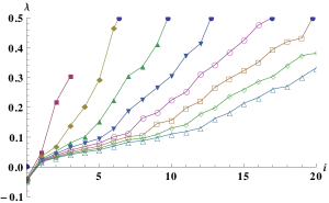
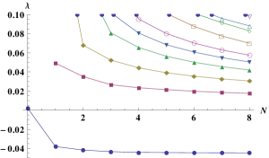
Figure 2: The eigenvalues $\lambda$ of (119), for the background given by the ansatz (132) with $k=1$ and $U_{1}=U_{0}$, for different basis sizes $M=N=0,1,\dots,8$. In both plots, the vertical axis is $\lambda$. In the upper plot, the horizontal axis is the number $i$ of the eigenvalue, starting from $0$, and the different graphs correspond to the different resolutions. In the lower plot, the horizontal axis is resolution indicated by $N$, with $M=N$, and the different graphs show different eigenvalues.

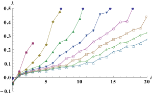
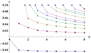
Figure 3: As before, but now for $k=1/2$.

In both examples, we have carried out the numerical integrations in $r$ for $M=N=8$. The results are similar in both examples. At all basis sizes up to and including this one, we find precisely one negative eigenvalue of $H$, as expected from the results of AkbarianChoptuik . Its value is $\lambda_{0}\simeq-0.045$ in both examples.

The approximate eigenvalues for different basis sizes are shown in Figs. 2 and 3. The lowest few eigenvalues appear to be converging with resolution to distinct values, providing evidence for the consistency of our method and a discrete spectrum.

The components $c^{mn}$ of the lowest eigenvector $\psi_{0}$ also seem to converge with $N$, but to diverge with $M$. The reason may be that the simple powers of $r-r_{3}$ and $Q-U_{1}$ are not good basis functions. The corresponding eigenfunctions appear visually to be smooth and converging with $M=N$ up to $M=N=7$. (In the $k=1/2$ example, $\psi_{0}$ diverges as expected, and this statement refers to $\sqrt{U_{0}-Q}\,\psi_{0}$, which is finite.) For the largest basis $M=N=8$, $\psi_{0}$ becomes noisy. Hence there is no point in increasing $M$ or $N$ beyond $M=N=8$ with our limited accuracy.

If we write the dynamics of the time-dependent perturbations as $-\psi_{,tt}=H\psi$, and $\lambda_{0}$ is the single negative eigenvalue of $H$, then the single unstable mode has time-dependence $\exp(\sqrt{-\lambda_{0}}t)$. This must correspond to $\exp(\tau/\sigma)$ in the notation of AkbarianChoptuik , where $\tau$ is the proper time at the centre. $\tau$ is related to our coordinate time $t$ (proper time at infinity) by $d\tau=\alpha_{c}\,dt$, where $\alpha_{c}$ is the lapse at the centre, and hence we have

$$\sigma={\alpha_{c}\over\sqrt{-\lambda_{0}}}.$$ (136)

With $\alpha_{c}\simeq 0.2968$ and $\lambda_{0}\simeq-0.0446$ for the $k=1$ background solution, and $\alpha_{c}\simeq 0.2874$ and $\lambda_{0}\simeq-0.0445$ for $k=1/2$, the formula (136) gives $\sigma\simeq 1.41$ and $1.36$, respectively, both compatible with the range $\sigma\simeq 1.43\pm 0.07$ given by AkbarianChoptuik .

However, we have implemented our numerics using only standard ODE solvers and nonlinear equations solvers (for solving the background equations by shooting) and numerical integration and linear algebra methods (for applying the Ritz method to the perturbations) in Mathematica, and have not tried to estimate our numerical error or optimise our methods.

V Conclusions

Numerical time evolutions of the Einstein-Vlasov system in spherical symmetry with massless particles AkbarianChoptuik have suggested the rather surprising conjecture that all static solutions of this system are one-mode unstable, with the time evolutions resulting in collapse for one sign of the initial amplitude of this mode, and dispersion for the other. In the language of critical phenomena in gravitational collapse, all static solutions are critical solutions at the threshold of collapse.

In Paper I paperI we have characterised all static solutions with massive particles in terms of a single function of two variables $k(Q,F)$. Here $F$ is essentially conserved angular momentum, and $Q$ essentially conserved energy per angular momentum, such that the orbit of a massless particle of given $Q$ and $F$ depends on $Q$ alone. Correspondingly, we have the degeneracy that all distributions $k(Q,F)$ of massless particles with the same $\bar{k}(Q):=\int k(Q,F)\,FdF$ give rise to the same spacetime.

In the current Paper II we have reduced the perturbations of static solutions (in spherical symmetry, with either massive or massless particles) to a single master variable $\psi(t,r,Q,F)$, which obeys an equation of motion of the form $-\psi_{,tt}=(H_{0}+H_{1})\psi$. In the massless case we have the same degeneracy for the perturbations as for the background, that is the metric perturbations only depend on $\bar{\psi}=\int\psi\,FdF$, but in contrast to the background equations this does simplify the equations significantly. Hence we have assumed $m\geq 0$ in most of this paper.

The kinetic part $H_{0}$ of $H$ is such that $\psi_{,tt}=H_{0}\psi$ is simply a second-order wave equation with characteristic speeds $\pm V(r,Q,F)$. There is no underlying wave equation in three space dimensions here. Rather, the left and right-going waves correspond to particles moving inwards and outwards in the background spacetime, with $V$ their radial velocity.

By contrast, the gravitational part $H_{1}$ of $H$ vanishes in the vacuum regions of the background solutions, and contains integrals over $Q$ and $F$ (as well as first $r$-derivatives) representing the gravitational pull of all the other particles represented by the perturbation $\psi$.

Following a suggestion by Olivier Sarbach, we have identified an inner product of perturbations $\psi$ which is positive definite for suitable background solutions and with respect to which the operator $H$ is symmetric. This additional mathematical structure allows us to find approximate eigenvectors $\psi$ and eigenvalues $\lambda$ of $H$ using the Ritz method. We have carried out the numerical procedure for two representative background solutions with massless particles (see Paper I for a discussion of these solutions and their significance), and we have found numerical evidence for a discrete spectrum of $\lambda$ with, for both backgrounds, a single negative eigenvalue with a value compatible with that found by Akbarian and Choptuik AkbarianChoptuik .

On the analytic side, we have characterised the space of functions $\psi(r,Q,F)$ as ${\mathbb{V}}=\hat{\mathbb{V}}\oplus\bar{\mathbb{V}}$, where a certain integral ${\cal I}\psi$ over $F$ and $Q$ vanishes for functions in $\hat{\mathbb{V}}$, while $\bar{\mathbb{V}}$ consists of functions of the form $f(r)X(r,Q,F)$ for a specific $X$ given by the background solution. Hence $\hat{\mathbb{V}}$ is infinitely larger than $\bar{\mathbb{V}}$. Unfortunately, eigenvectors $\psi$ of $H$ cannot lie entirely in either subspace. We have also found that we can write $H$ as the difference of two squares, $H=A^{\dagger}A-D^{\dagger}D$, with $D=D^{\dagger}$ annihilating $\hat{\mathbb{V}}$. Unfortunately, the commutators of $A^{\dagger}$, $A$ and $D$ are not simple, and so the apparent analogy with the quantisation of the harmonic oscillator does not seem to be helpful.

We had hoped that in bringing the perturbation equations into a sufficiently simple form we could prove the conjecture of AkbarianChoptuik that every spherically symmetric static solution with massless particles has precisely one unstable mode and/or calculate its value in closed form. We had also hoped to be able to show that some spherically symmetric static solutions with massive particles are stable, as conjectured in AndreassonRein2006 . We have not been able to do either, but hope that our formulation of the problem will be of future use.

- (1) G. Rein and A.D. Rendall, Commun. Math. Phys. 150, 561 (1992).
- (2) M. Dafermos J. Hyperbol. Differ. Equations 3, 589 (2006).
- (3) J.M. Martín-García and C. Gundlach, Phys. Rev. D 65, 084026, 1 (2002).
- (4) A.D. Rendall and J.J.L. Velazquez, Annales Henri Poincaré 12, 919 (2011).
- (5) G. Rein and A.D. Rendall Math. Proc. Camb. Phil. Soc. 128, 363 (2000).
- (6) H. Andréasson and G. Rein, Class. Quantum Grav. 23, 3659 (2006).
- (7) C. Gundlach, Phys. Rev. D 94, 124046 (2016).
- (8) H. Andréasson, Living Reviews in Relativity 2011-4 (2011).
- (9) A. Akbarian and M. W. Choptuik, Phys. Rev. D 90, 104023 (2014).
- (10) J. Schaeffer, Commun. Math. Phys. 204, 313 (1999).
- (11) H. DeJonghe, Phys. Rep. 133, 217 (1986).