11	Orbital Physics
	Andrzej M. Oleś
	Marian Smoluchowski Institute of Physics
Jagiellonian University
	Prof. S. Łojasiewicza 11, Kraków, Poland

1 Introduction: strong correlations at orbital degeneracy

Strong local Coulomb interactions lead to electron localization in Mott or charge transfer correlated insulators. The simplest model of a Mott insulator is the non-degenerate Hubbard model where large intraorbital Coulomb interaction $U$ suppresses charge fluctuations due to the kinetic energy $\propto t$. As a result, the physical properties of a Mott insulator are determined by an interplay of kinetic exchange $\propto J$, with

$$J=\frac{4t^{2}}{U},$$ (1)

derived from the Hubbard model at $U\gg t$, and the motion of holes in the restricted Hilbert space without double occupancies, as described by the $t$-$J$ model [1]. Although this generic model captures the essential idea of strong correlations, realistic correlated insulators arise in transition metal oxides (or fluorides) and the degeneracy of partly filled and nearly degenerate $3d$ (or $4d$) strongly correlated states has to be treated explicitly. Quite generally, strong local Coulomb interactions lead then to the multitude of quite complex behavior with often puzzling transport and magnetic properties [2]. The theoretical understanding of this class of compounds, including the colossal magneto-resistance (CMR) manganites as a prominent example [3], has to include not only spins and holes but in addition orbital degrees of freedom which have to be treated on equal footing with the electron spins [4]. For a Mott insulator with transition metal ions in $d^{m}$ configurations, charge excitations along the bond $\langle ij\rangle$, $d_{i}^{m}d_{j}^{m}\rightleftharpoons d_{i}^{m+1}d_{j}^{m-1}$, lead to spin-orbital superexchange which couples two neighboring ions at sites $i$ and $j$.

It is important to realize that modeling of transition metal oxides can be performed on different levels of sophistication. We shall present some effective orbital and spin-orbital superexchange models for the correlated $3d$-orbitals depicted in Fig. 1 coupled by hopping $t$ between nearest neighbor ions on a perovskite lattice, while the hopping for other lattices may be generated by the general rules formulated by Slater and Koster [5]. The orbitals have particular shapes and belong to two irreducible representations of the $O_{h}$ cubic point group: ($i$) a two-dimensional (2D) representation of $e_{g}$-orbitals $\{3z^{2}-r^{2},x^{2}-y^{2}\}$, and ($ii$) a three-dimensional (3D) representation of $t_{2g}$-orbitals $\{xy,yz,zx\}$. In case of absence of any tetragonal distortion or crystal-field due to surrounding oxygens, the $3d$-orbitals are degenerate within each irreducible representation of the $O_{h}$ point group and have typically a large splitting $10D_{q}\sim~{}2.0$ eV between them. When such degenerate orbitals are party filled, electrons (or holes) have both spin and orbital degree of freedom. The kinetic energy $H_{t}$ in a perovskite follows from the hybridization between $3d$ and $2p$-orbitals. In an effective $d$-orbital model the oxygen $2p$-orbitals are not included explicitly and we define the hopping element $t$ as the largest hopping element obtained for two orbitals of the same type which belong to the nearest neighbor $3d$ ions.

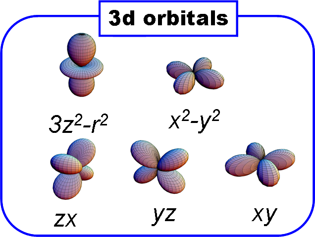
Fig. 1: Schematic representation of $3d$ orbitals: Top — two $e_{g}$ orbitals $\{3z^{2}-r^{2},x^{2}-y^{2}\}$; Bottom — three $t_{2g}$ orbitals $\{zx,yz,xy\}$. Image by courtesy of Yoshinori Tokura.

We begin with conceptually simpler $t_{2g}$ orbitals where finite hopping $t$ results from the ${d-p}$ hybridization along $\pi$-bonds and couples each a pair of identical orbitals active along a given bond. Each $t_{2g}$ orbital is active along two cubic axes and the hopping is forbidden along the one perpendicular to the plane of this orbital, e.g. the hopping between two $xy$-orbitals is not allowed along the $c$ axis (due to the cancelations caused by orbital phases). It is therefore convenient to introduce the following short-hand notation for the orbital degree of freedom [6],

$$|a\rangle\equiv|yz\rangle,\hskip 19.91684pt|b\rangle\equiv|zx\rangle,\hskip 19.91684pt|c\rangle\equiv|xy\rangle.$$ (2)

The labels $\gamma=a,b,c$ thus refer to the cubic axes where the hopping is absent for orbitals of a given type,

$$H_{t}(t_{2g})=-t\sum_{\alpha}\sum_{\langle ij\rangle\parallel\gamma\neq\alpha}a_{i\alpha\sigma}^{\dagger}a_{j\alpha\sigma},$$ (3)

Here $a^{\dagger}_{i\alpha\sigma}$ is an electron creation operator in a $t_{2g}$-orbital $\alpha\in\{xy,yz,zx\}$ with spin $\sigma=\uparrow,\downarrow$ at site $i$, and the local electron density operator for a spin-orbital state is $n_{i\alpha\sigma}=a^{\dagger}_{i\alpha\sigma}a_{i\alpha\sigma}$. Not only spin but also orbital flavor is conserved in the hopping process $\propto t$.

The hopping Hamiltonian for $e_{g}$ electrons couples two directional $e_{g}$-orbitals $\{|i\zeta_{\alpha}\rangle,|i\zeta_{\alpha}\rangle\}$ along a $\sigma$-bond $\left\langle ij\right\rangle$ [7],

$$H_{t}(e_{g})=-t\sum_{\alpha}\sum_{\langle ij\rangle\parallel\alpha,\sigma}a_{i\zeta_{\alpha}\sigma}^{\dagger}a_{j\zeta_{\alpha}\sigma}.$$ (4)

Indeed, the hopping with amplitude $-t$ between sites $i$ and $j$ occurs only when an electron with spin $\sigma$ transfers between two directional orbitals $|\zeta_{\alpha}\rangle$ oriented along the bond $\langle ij\rangle$ direction, i.e., $|\zeta_{\alpha}\rangle\propto 3x^{2}-r^{2}$, $3y^{2}-r^{2}$, and $3z^{2}-r^{2}$ along the cubic axis $\alpha=a$, $b$, and $c$. We will similarly denote by $|\xi_{\alpha}\rangle$ the orbital which is orthogonal to $|\zeta_{\alpha}\rangle$ and is oriented perpendicular to the bond $\langle ij\rangle$ direction, i.e., $|\xi_{\alpha}\rangle\propto y^{2}-z^{2}$, $z^{2}-x^{2}$, and $x^{2}-y^{2}$ along the axis $\alpha=a$, $b$, and $c$. For a moment we consider only electrons with one spin, $\sigma=\uparrow$, to focus on the orbital problem. While such a choice of an over-complete basis $\{\zeta_{a},\zeta_{b},\zeta_{c}\}$ is convenient for writing down the kinetic energy, a particular orthogonal basis is needed. The usual choice is to take

$$\textstyle{|z\rangle\equiv\frac{1}{\sqrt{6}}(3z^{2}-r^{2}),\hskip 19.91684pt|\bar{z}\rangle\equiv\frac{1}{\sqrt{2}}(x^{2}-y^{2}),}$$ (5)

called real $e_{g}$ orbitals [7]. However, this basis is the natural one only for the bonds parallel to the $c$ axis but not for those in the $(a,b)$ plane, and for $\uparrow$-spin electrons the hopping reads (here for clarity we omit spin index $\sigma$)

$$H_{t}^{\uparrow}(e_{g})=-\frac{1}{4}t\!\sum_{\langle ij\rangle\parallel ab}\!\left[3a_{i\bar{z}}^{\dagger}a_{j\bar{z}}+a_{iz}^{\dagger}a_{jz}\mp\sqrt{3}\left(a_{i\bar{z}}^{\dagger}a_{jz}+a_{iz}^{\dagger}a_{j\bar{z}}\right)\right]-t\sum_{\langle ij\rangle\parallel c}a_{iz}^{\dagger}a_{jz},$$ (6)

and although this expression is of course cubic invariant, it does not manifest this symmetry but takes a very different appearance depending on the bond direction. However, the symmetry is better visible using the basis of complex $e_{g}$ orbitals at each site $j$ [7],

$$\textstyle{|j+\rangle=\frac{1}{\sqrt{2}}\big{(}|jz\rangle-i|j\bar{z}\rangle\big{)},\hskip 19.91684pt|j-\rangle=\frac{1}{\sqrt{2}}\big{(}|jz\rangle+i|j\bar{z}\rangle\big{)},}$$ (7)

corresponding to “up” and“down” pseudospin flavors, with the local pseudospin operators defined as

$$\tau_{i}^{+}\equiv c_{i+}^{\dagger}c_{i-},\hskip 19.91684pt\tau_{i}^{-}\equiv c_{i-}^{\dagger}c_{i+},\hskip 19.91684pt\tau_{i}^{z}\equiv\textstyle{\frac{1}{2}}(c_{i+}^{\dagger}c_{i+}-c_{i-}^{\dagger}c_{i-})=\textstyle{\frac{1}{2}}(n_{i+}-n_{i-}).$$ (8)

The three directional $|i\zeta_{\alpha}\rangle$ and three planar $|i\xi_{\alpha}\rangle$ orbitals at site $i$, associated with the three cubic axes ($\alpha=a$, $b$, $c$), are the real orbitals,

$$|i\zeta_{\alpha}\rangle = \textstyle{\frac{1}{\sqrt{2}}}\,\left[e^{-i\vartheta_{\alpha}/2}|i+\rangle+e^{+i\vartheta_{\alpha}/2}|i-\rangle\right]=\cos(\vartheta_{\alpha}/2)|iz\rangle-\sin(\vartheta_{\alpha}/2)|i\bar{z}\rangle,$$ (9)

$$|i\xi_{\alpha}\rangle = \textstyle{\frac{1}{\sqrt{2}}}\,\left[e^{-i\vartheta_{\alpha}/2}|i+\rangle-e^{+i\vartheta_{\alpha}/2}|i-\rangle\right]=\sin(\vartheta_{\alpha}/2)|iz\rangle+\cos(\vartheta_{\alpha}/2)|i\bar{z}\rangle,$$ (10)

with the phase factors $\vartheta_{ia}=-4\pi/3$, $\vartheta_{ib}=+4\pi/3$, and $\vartheta_{ic}=0$, and thus correspond to the pseudospin lying in the equatorial plane and pointing in one of the three equilateral “cubic” directions defined by the angles $\{\vartheta_{i\alpha}\}$.

Using the above complex-orbital representation (7) we can write the orbital Hubbard model for $e_{g}$ electrons with only one spin flavor $\sigma=\uparrow$ in a form similar to the spin Hubbard model,

$${\cal H}^{\uparrow}(e_{g})=-\frac{1}{2}t\sum_{\alpha}\!\sum_{\langle ij\rangle\parallel\alpha}\Big{[}\Big{(}a_{i+}^{\dagger}a_{j+}+a_{i-}^{\dagger}a_{j-}\Big{)}+\gamma\Big{(}e^{-i\chi_{\alpha}}a_{i+}^{\dagger}a_{j-}+e^{+i\chi_{\alpha}}a_{i-}^{\dagger}a_{j+}\Big{)}\Big{]}+\,\bar{U}\sum_{i}n_{i+}n_{i-},$$ (11)

with $\chi_{a}=+2\pi/3$, $\chi_{b}=-2\pi/3$, and $\chi_{c}=0$, and where the parameter $\gamma$, explained below, takes for $e_{g}$ orbitals the value $\gamma=1$. The appearance of the phase factors $e^{\pm i\chi_{\alpha}}$ is characteristic of the orbital problem — they occur because the orbitals have an actual shape in real space so that each hopping process depends on the bond direction and may change the orbital flavor. The interorbital Coulomb interaction $\propto\bar{U}$ couples the electron densities in basis orbitals ${n_{i\alpha}=a_{i\mu}^{\dagger}a_{i\mu}}$, with $\mu\in\{+,-\}$; its form in invariant under any local basis transformation to a pair of orthogonal orbitals, i.e., it gives an energy $\bar{U}$ for a double occupancy either when two real orbitals are simultaneously occupied, $\bar{U}\sum_{i}n_{iz}n_{i\bar{z}}$, or when two complex orbitals are occupied, $\bar{U}\sum_{i}n_{i+}n_{i-}$.

In general, on-site Coulomb interactions between two interacting electrons in $3d$-orbitals depend both on spin and orbital indices and the interaction Hamiltonian takes the form of the degenerate Hubbard model. Note that the electron interaction parameters in this model are effective ones, i.e., the $2p$-orbital parameters of O (F) ions renormalize on-site Coulomb interactions for $3d$-orbitals. The general form which includes only two-orbital interactions and the anisotropy of Coulomb and exchange elements is [8]:

$$H_{int} = U\sum_{i\alpha}n_{i\alpha\uparrow}n_{i\alpha\downarrow}+\sum_{i,\alpha<\beta}\left(U_{\alpha\beta}-\frac{1}{2}J_{\alpha\beta}\right)\,n_{i\alpha}n_{i\beta}-2\sum_{i,\alpha<\beta}J_{\alpha\beta}\,{\vec{S}}_{i\alpha}\cdot{\vec{S}}_{i\beta}$$ (12)

$$+ \sum_{i,\alpha<\beta}J_{\alpha\beta}\left(a^{\dagger}_{i\alpha\uparrow}a^{\dagger}_{i\alpha\downarrow}a_{i\beta\downarrow}a_{i\beta\uparrow}+a^{\dagger}_{i\beta\uparrow}a^{\dagger}_{i\beta\downarrow}a_{i\alpha\downarrow}a_{i\alpha\uparrow}\right).$$

Here $a^{\dagger}_{i\alpha\sigma}$ is an electron creation operator in any $3d$-orbital $\alpha\in\{xy,yz,zx,3z^{2}-r^{2},x^{2}-y^{2}\}$ and $\bar{\sigma}equiv-\sigma$, with spin states $\sigma=\uparrow,\downarrow$ at site $i$. The parameters $\{U,U_{\alpha\beta},J_{\alpha\beta}\}$ depend in the general case on the three Racah parameters $A$, $B$ and $C$ [9] which may be derived from somewhat screened atomic values. While the intraorbital Coulomb element is identical for all $3d$-orbitals,

$$U=A+4B+3C$$ (13)

the interorbital Coulomb $U_{\alpha\beta}$ and exchange $J_{\alpha\beta}$ elements are anisotropic and depend on the involved pair of orbitals; the values of $J_{\alpha\beta}$ are given in Table 1. The Coulomb $U_{\alpha\beta}$ and exchange $J_{\alpha\beta}$ elements are related to the intraorbital element $U$ by a relation which guarantees the invariance of interactions in the orbital space,

$$U=U_{\alpha\beta}+2J_{\alpha\beta}.$$ (14)

Table 1: On-site interorbital exchange elements $J_{\alpha\beta}$ for $3d$ orbitals as functions of the Racah parameters $B$ and $C$ (for more details see Ref. [9]).

$3d$ orbital	$xy$	$yz$	$zx$	$x^{2}-y^{2}$	$3z^{2}-r^{2}$
$xy$	$0$	$3B+C$	$3B+C$	$C$	$4B+C$
$yz$	$3B+C$	$0$	$3B+C$	$3B+C$	$B+C$
$zx$	$3B+C$	$3B+C$	$0$	$3B+C$	$B+C$
$x^{2}-y^{2}$	$C$	$3B+C$	$3B+C$	$0$	$4B+C$
$3z^{2}-r^{2}$	$4B+C$	$B+C$	$B+C$	$4B+C$	$0$

In all situations where only the orbitals belonging to a single irreducible representation of the cubic group ($e_{g}$ or $t_{2g}$) are partly filled, as e.g. in the titanates, vanadates, nickelates, or copper fluorides, the filled (empty) orbitals do not contribute, and the relevant exchange elements $J_{\alpha\beta}$ are all the same (see Table 1), i.e., for $t_{2g}$ ($e_{g}$) orbitals,

$$J_{H}^{t} = 3B+C,$$ (15)

$$J_{H}^{e} = 4B+C.$$ (16)

Then one may use a simplified degenerate Hubbard model with isotropic form of on-site interactions (for a given subset of $3d$ orbitals) [10],

$$H_{int}^{(0)} = U\sum_{i\alpha}n_{i\alpha\uparrow}n_{i\alpha\downarrow}+\left(U-\frac{5}{2}J_{H}\right)\sum_{i,\alpha<\beta}n_{i\alpha}n_{i\beta}-2J_{H}\sum_{i,\alpha<\beta}\,\vec{S}_{i\alpha}\cdot\vec{S}_{i\beta}$$ (17)

$$+ J_{H}\sum_{i,\alpha<\beta}\left(a^{\dagger}_{i\alpha\uparrow}a^{\dagger}_{i\alpha\downarrow}a_{i\beta\downarrow}a_{i\beta\uparrow}+a^{\dagger}_{i\beta\uparrow}a^{\dagger}_{i\beta\downarrow}a_{i\alpha\downarrow}a_{i\alpha\uparrow}\right).$$

It has two Kanamori parameters: the Coulomb intraorbital element $U$ (13) and Hund’s exchange $J_{H}$ standing either for $J_{H}^{t}$ (15) or for $J_{H}^{e}$ (16). Now $\bar{U}\equiv(U-3J_{H})$ in Eq. (11). We emphasize that in a general case when both types of orbitals are partly filled (as in the CMR manganites) and both thus participate in charge excitations, the above Hamiltonian with a single Hund’s exchange element $J_{H}$ is insufficient and the full anisotropy given in Eq. (17) has to be used instead to generate correct charge excitation spectra of a given transition metal ion [9].

2 Orbital and compass models

If the spin state is ferromagnetic (FM) as e.g. in the $ab$ planes of KCuF₃ (or LaMnO₃), charge excitations $d_{i}^{m}d_{j}^{m}\rightleftharpoons d_{i}^{m+1}d_{j}^{m-1}$ with $m=9$ (or $m=4$) concern only high-spin (HS) ${}^{3}A_{1}$ (or ${}^{6}A_{1}$) state and the superexchange interactions reduce to an orbital superexchange model [11]. Thus we begin with an orbital model for $e_{g}$-holes in K₂CuF₄, with a local basis at site $i$ defined by two real $e_{g}$-orbitals, see Eq. (5), being a local $e_{g}$-orbital basis at each site. The basis consists of a directional orbital $|i\zeta_{c}\rangle\equiv|iz\rangle$ and the planar orbital $|i\xi_{c}\rangle\equiv|i\bar{z}\rangle$. Other equivalent orbital bases are obtained by rotation of the above pair of orbitals by angle $\vartheta$ to

$$|i\vartheta\rangle = \cos\left(\vartheta/2\right)|iz\rangle-\sin\left(\vartheta/2\right)|i\bar{z}\rangle,$$

$$|i\bar{\vartheta}\rangle = \sin\left(\vartheta/2\right)|iz\rangle+\cos\left(\vartheta/2\right)|i\bar{z}\rangle,$$ (18)

i.e., to a pair $\{|i\vartheta\rangle,|i,\vartheta+\pi\rangle\}$. For angles $\vartheta=\pm 4\pi/3$ one finds equivalent pairs of directional and planar orbitals in a 2D model, $\{|i\zeta_{a}\rangle,|i\xi_{a}\rangle\}$ and $\{|i\zeta_{b}\rangle,|i\xi_{b}\rangle\}$, to the usually used  $e_{g}$-orbital real basis given by Eq. (5).

Consider now a bond $\langle ij\rangle\!\parallel\!\gamma$ along one of the cubic axes $\gamma=a,b,c$, and a charge excitation generated by a hopping process $i\rightarrow j$. The hopping $t$ couples two directional orbitals $\{|i\zeta_{\gamma}\rangle,|j\zeta_{\gamma}\rangle\}$. Local projection operators on these active and the complementary inactive $\{|i\xi_{\gamma}\rangle,|j\xi_{\gamma}\rangle\}$ orbitals are

$${\cal P}_{i\zeta}^{\gamma}=|i\zeta_{\gamma}\rangle\langle i\zeta_{\gamma}|=\left(\frac{1}{2}+\tau^{(\gamma)}_{i}\right),\hskip 19.91684pt{\cal P}_{i\xi}^{\gamma}=|i\xi_{\gamma}\rangle\langle i\xi_{\gamma}|=\left(\frac{1}{2}-\tau^{(\gamma)}_{i}\right),$$ (19)

where

$$\tau^{(\gamma)}_{i}\equiv\,\frac{1}{2}\,\left(|i\zeta_{\gamma}\rangle\langle i\zeta_{\gamma}|-|i\xi_{\gamma}\rangle\langle i\xi_{\gamma}|\right),$$ (20)

and these operators are represented in the fixed $\{|iz\rangle,|i\bar{z}\rangle\}$ basis as follows:

$$\tau^{(a)}_{i}=-\frac{1}{4}\left(\sigma^{z}_{i}-\sqrt{3}\sigma^{x}_{i}\right),\hskip 19.91684pt\tau^{(b)}_{i}=-\frac{1}{4}\left(\sigma^{z}_{i}+\sqrt{3}\sigma^{x}_{i}\right),\hskip 19.91684pt\tau^{(c)}_{i}=\frac{1}{2}\sigma^{z}_{i}.$$ (21)

A charge excitation between two transition metal ions with partly filled $e_{g}$-orbitals will arise by a hopping process between two active orbitals, $|i\zeta_{\gamma}\rangle$ and $|j\zeta_{\gamma}\rangle$. To capture such processes we introduce two projection operators on the orbital states for each bond,

$${\cal P}_{\langle ij\rangle}^{(\gamma)} \equiv \left(\frac{1}{2}+\tau^{(\gamma)}_{i}\right)\left(\frac{1}{2}-\tau^{(\gamma)}_{j}\right)+\left(\frac{1}{2}-\tau^{(\gamma)}_{i}\right)\left(\frac{1}{2}+\tau^{(\gamma)}_{j}\right),$$ (22)

$${\cal Q}_{\langle ij\rangle}^{(\gamma)} \equiv 2\left(\frac{1}{2}-\tau^{(\gamma)}_{i}\right)\left(\frac{1}{2}-\tau^{(\gamma)}_{j}\right).$$ (23)

Unlike for a spin system, the charge excitation $d_{i}^{m}d_{j}^{m}\rightleftharpoons d_{i}^{m+1}d_{j}^{m-1}$ is allowed only in one direction when one orbital is directional $|\zeta_{\gamma}\rangle$ and the other is planar $|\xi_{\gamma}\rangle$ on the bond $\langle ij\rangle\parallel\gamma$, i.e., $\left\langle{\cal P}_{\langle ij\rangle}^{(\gamma)}\right\rangle=1$; such processes generate both HS and low-spin (LS) contributions. On the contrary, when both orbitals are directional, i.e., one has $\left\langle{\cal Q}_{\langle ij\rangle}^{(\gamma)}\right\rangle=2$, only LS terms contribute.

(c)

Fig. 2: Virtual charge excitations leading to the $e_{g}$ orbital superexchange model for a strongly correlated system with $|z\rangle$ and $|x\rangle\equiv|\bar{z}\rangle$ real $e_{g}$ orbitals (5) in the subspace of $\uparrow$-spin states: (a) for a bond along the $c$ axis $\langle ij\rangle\parallel c$; (b) for a bond in the $ab$ plane $\langle ij\rangle\parallel ab$. In a FM plane of KCuF₃ (LaMnO₃) the superexchange (27) favors (c) AO state of $|{\rm AO}\pm\rangle$ orbitals (28). Images (a-b) are reproduced from Ref. [11]; image (c) by courtesy of Krzysztof Bieniasz.

To write the superexchange model we need the charge excitation energy which for the HS channel is,

$$\varepsilon_{1}\equiv E_{1}(d^{m+1})+E_{0}(d^{m-1})-2E_{0}(d^{m})=U-3J_{H}=\bar{U},$$ (24)

where $E_{0}(d^{m})$ in the ground state energy for an ion with $m$ electrons. Note that this energy is the same for KCuF₃ and LaMnO₃ [8], so the $e_{g}$ orbital model presented here is universal. Second order perturbation theory shown in Figs. 2(a-b) gives [11],

$${\cal H}^{\uparrow}(e_{g})=-\frac{t^{2}}{\varepsilon_{1}}\sum_{\langle ij\rangle\parallel\gamma}{\cal P}_{\langle ij\rangle}^{(\gamma)}.$$ (25)

For convenience we define the dimensionless Hund’s exchange parameter $\eta$,

$$\eta \equiv \frac{J_{H}}{U}.$$ (26)

The value of $J$ defines the superexchange energy scale and is the same as in the $t$-$J$ model [1], while the parameter $\eta$ (26) characterizes the multiplet structure when LS states are included as well, see below. The $e_{g}$ orbital model (25) (for HS states) takes the form,

$${\cal H}^{\uparrow}(e_{g})=\frac{1}{2}Jr_{1}\sum_{\langle ij\rangle\parallel\gamma}\left(\tau^{(\gamma)}_{i}\tau^{(\gamma)}_{j}-\frac{1}{4}\right)+E_{z}\sum_{i}\tau_{i}^{(c)},$$ (27)

where $r_{1}=U/\varepsilon_{\rm HS}=U/\bar{U}=1/(1-3\eta)$. Here we include the crystal-field term $\propto E_{z}$ which splits off the $e_{g}$ orbitals. The same effective model is obtained from the $e_{g}$ Hubbard model Eq. (11) at half-filling in the regime of $\bar{U}\gg t$. It favors consistently with its derivation pairs of orthogonal orbitals along the axis $\gamma$, with the energy gain for such a configuration $-\frac{1}{4}Jr_{1}$. When both orbitals would be instead selected as directional along the bond, $\left\langle\tau^{(\gamma)}_{i}\tau^{(\gamma)}_{j}\right\rangle=\frac{1}{4}$, the energy gain vanishes as this orbital configuration corresponds to the situation incompatible with the HS excited states considered here and the superexchange is blocked. The ground state in the 2D $ab$ plane has alternating orbital (AO) order between the sublattices $i\in A$ and $j\in B$,

$$\textstyle{|i+\rangle=\frac{1}{\sqrt{2}}\big{(}|iz\rangle+|i\bar{z}\rangle\big{)},\hskip 19.91684pt|j-\rangle=\frac{1}{\sqrt{2}}\big{(}|jz\rangle-|j\bar{z}\rangle\big{)},}$$ (28)

of orbitals occupied by holes in KCuF₃ and by electrons in LaMnO₃, see Fig. 2(c).

(a-b)   (c)

Fig. 3: (a-b) Orbital-wave excitations obtained for different values of the crystal-field splitting $E_{z}$ for a 3D (left) and 2D (right) orbital superexchange model (27), with $Jr_{1}\equiv J$. The result shown for a 3D model at $E_{z}=0$ corresponds to the $E_{z}\to 0$ limit. (c) Gap $\Delta/J$ in the orbital excitation spectrum and energy quantum correction $\Delta E/J$ as functions of the crystal-field splitting $E_{z}/J$, for the 3D (2D) model shown by full (dashed) lines. Images are reproduced from Ref. [11].

Here we are interested in the low temperature range $T<0.1J$ and the 2D (and 3D) $e_{g}$ orbital model orders at finite temperature $T<T_{c}$ [12], i.e., below $T_{c}=0.3566J$ for a 2D model [13], so we assume perfect orbital order given by a classical Ansatz for the ground state,

$$|\Phi_{0}\rangle=\prod_{i\in A}|i\theta_{A}\rangle\prod_{j\in B}|j\theta_{B}\rangle,$$ (29)

with the orbital states, $|i\theta_{A}\rangle$ and $|j\theta_{B}\rangle$, characterized by opposite angles ($\theta_{A}=-\theta_{B}$) and alternating between two sublattices $A$ and $B$ in the $ab$ planes. The orbital state at site $i$:

$$|i\theta\rangle=\cos\left(\theta/2\right)|iz\rangle+\sin\left(\theta/2\right)|i\bar{z}\rangle,$$ (30)

is here parameterized by an angle $\theta$ which defines the amplitudes of the orbital states defined in Eq. (5). The AO state specified in Eq. (29) is thus defined by:

$$|i\theta_{A}\rangle = \cos\left(\theta/2\right)|iz\rangle+\sin\left(\theta/2\right)|ix\rangle,$$

$$|j\theta_{B}\rangle = \cos\left(\theta/2\right)|jz\rangle-\sin\left(\theta/2\right)|jx\rangle,$$ (31)

with $\theta_{A}=\theta$ and $\theta_{B}=-\theta$.

The excitations from the ground state of the orbital model (27) are orbital waves (orbitons) which may be obtained in a similar way to magnons in a quantum antiferromagnet. An important difference is that the orbitons have two branches which are in general nondegenerate, see Fig. 3(a-b). In the absence of crystal field ($E_{z}=0$) the spectrum for the 2D $e_{g}$ orbital model has a gap and the orbitons have weak dispersion, so the quantum corrections to the order parameter are rather small. They are much larger in the 3D model but still smaller than in an antiferromagnet [11]. The gap closes in the 3D model at $E_{z}=0$, but the quantum corrections are smaller than in the Heisenberg model. Note that the shape of the occupied orbitals changes at finite crystal field, and the orbitons have a remarkable evolution, both in the 3D and 2D model, see Figs. 3(a-b). Increasing $E_{z}>0$ first increases the gap but when the field overcomes the interactions and polarizes the orbitals (at $E_{z}=4J$ in 2D and $E_{z}=6J$ in 3D model), the gap closes, see Fig. 3(c). This point marks a transition from the AO order to uniform ferro-orbital (FO) order. Note that in agreement with intuition the quantum corrections $\Delta E/J$ are maximal when the gap closes and low-energy orbitons contribute.

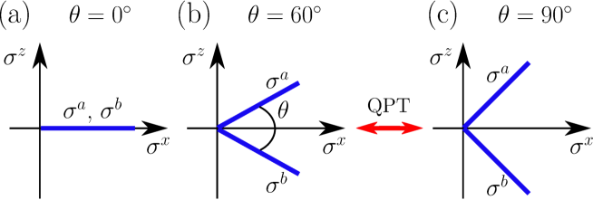
Fig. 4: Artist’s view of the evolution of orbital interactions in the generalized compass model Eq. (32) with increasing angle $\theta$. Heavy (blue) lines indicate favored spin direction induced by interactions along two nonequivalent lattice axes $a$ and $b$. Different panels show: (a) the Ising model at $\theta=0^{\circ}$, (b) the 2D $e_{g}$ orbital model at $\theta=60^{\circ}$, and (c) the OCM at $\theta=90^{\circ}$. Spin order follows the interactions in the Ising limit, while it follows one of the equivalent interactions, $\sigma^{a}$ or $\sigma^{b}$, in the OCM. This results in the symmetry breaking quantum phase transition (QPT) which occurs between (b) and (c). Image is reproduced from Ref. [15].

To see the relation of the 2D $e_{g}$ orbital model to the compass model [14] we introduce a 2D generalized compass model (GCM) with pseudospin interactions on a square lattice in $ab$ plane ($J_{\rm cm}>0$) [15],

$${\cal H}(\theta)=-J_{\rm cm}\sum_{\{ij\}\in ab}\left\{\sigma^{a}_{ij}(\theta)\sigma^{a}_{i+1,j}(\theta)+\sigma^{b}_{ij}(\theta)\sigma^{b}_{i,j+1}(\theta)\right\}\,.$$ (32)

The interactions occur along nearest neighbor bonds and are balanced along both lattice directions $a$ and $b$. Here $\{ij\}$ labels lattice sites in the $ab$ plane and $\{\sigma^{a}_{ij}(\theta),\sigma^{b}_{ij}(\theta)\}$ are linear combinations of Pauli matrices describing interactions for $T=\frac{1}{2}$ pseudospins:

$$\sigma^{a}_{ij}(\theta)\! = \cos(\theta/2)\;\sigma^{x}_{ij}+\sin(\theta/2)\;\sigma^{z}_{ij}\,,$$

$$\sigma^{b}_{ij}(\theta)\! = \cos(\theta/2)\;\sigma^{x}_{ij}-\sin(\theta/2)\;\sigma^{z}_{ij}\,.$$ (33)

The interactions in Eq. (32) include the classical Ising model for $\sigma^{x}_{ij}$ operators at $\theta=0^{\circ}$ and become gradually more frustrated with increasing angle $\theta\in(0^{\circ},90^{\circ}]$ — they interpolate between the Ising model (at $\theta=0^{\circ}$) and the isotropic compass model (at $\theta=90^{\circ}$), see Fig. 4. The latter case is equivalent by a standard unitary transformation to the 2D compass model with standard interactions, $\sigma^{x}_{ij}\sigma^{x}_{i,j+1}$ along the $a$ and $\sigma^{z}_{ij}\sigma^{z}_{i+1,j}$ along the $b$ axis [15],

$${\cal H}(\pi/2)=-J_{\rm cm}\sum_{\langle ij\rangle\parallel a}\,\sigma^{x}_{ij}\sigma^{x}_{i+1,j}-J_{\rm cm}\sum_{\langle ij\rangle\parallel b}\,\sigma^{z}_{ij}\sigma^{z}_{i,j+1}\,.$$ (34)

The model (32) includes as well the 2D $e_{g}$ orbital model as a special case, i.e., at $\theta=60^{\circ}$. Increasing angle $\theta$ between the interacting orbital-like components (2) in Fig. 4 is equivalent to increasing frustration which becomes maximal in the 2D compass model. As a result, a second order quantum phase transition from Ising to nematic order [16] occurs at $\theta_{c}\simeq 84.8^{\circ}$ which is surprisingly close to the compass point $\theta=90^{\circ}$, i.e., only when the interactions are sufficiently strongly frustrated. The ground state has high degeneracy $d=2^{L+1}$ for a 2D cluster $L\times L$ of one-dimensional (1D) nematic states which are entirely different from the 2D AO order in the $e_{g}$ orbital model depicted in Fig. 4(c), yet it is stable in a range of temperature below $T_{c}\simeq 0.06J_{\rm cm}$ [17].

3 Superexchange models for active $e_{g}$ orbitals

3.1 General structure of the spin-orbital superexchange

We consider the case of partly filled degenerate $3d$-orbitals and large Hund’s exchange $J_{H}$. In the regime of $t\ll U$, electrons localize and effective low-energy superexchange interactions consist of all the contributions which originate from possible virtual charge excitations, $d_{i}^{m}d_{j}^{m}\rightleftharpoons d_{i}^{m+1}d_{j}^{m-1}$ — they take a form of a spin-orbital model, see Eq. (37) below. The charge excitation $n$ costs the energy

$$\varepsilon_{n}=E_{n}(d^{m+1})+E_{0}(d^{m-1})-2E_{0}(d^{m}),$$ (35)

where the $d^{m}$ ions are in the initial HS ground states with spins $S=\frac{m}{2}$ and have the Coulomb interaction energy $E_{0}(d^{m})={m\choose 2}(U-3J_{H})$ each (if $m<5$, else if $m>5$ one has to consider here $m$ holes instead, while the case of $m=5$ is special and will not be considered here as in the $t_{2g}^{3}e_{g}^{2}$ configuration the orbital degree of freedom is quenched). The same formula for ground state energy applies as well to Mn³⁺ ions in $d^{4}$ configuration with $S=2$ spin HS ground state, see Sec. 3.3. By construction also the ion with less electrons (holes) for $m<5$ is in the HS state and $E_{0}(d^{m-1})={m-1\choose 2}(U-3J_{H})$. The excitation energies (35) are thus defined by the multiplet structure of an ion with more electrons (holes) in the configuration $d^{m+1}$, see Fig. 5. The lowest energy excitation is given by Eq. (24) — it is obtained from the HS state of the $3d^{m+1}$ ion with total spin ${\cal S}=S+\frac{1}{2}$ and energy $E_{1}(d^{m+1})={m+1\choose 2}(U-3J_{H})$. Indeed, one recovers the lowest excitation energy in the HS subspace, see Eq. (24), with $J_{H}$ being Hund’s exchange element for the electron (hole) involved in the charge excitation, either $e_{g}$ or $t_{2g}$. We emphasize that this lowest excitation energy $\varepsilon_{1}$ (24) is universal and is found both in $t_{2g}$ and $e_{g}$ systems, i.e., it does not depend on the electron valence $m$. In contrast, the remaining energies $\{\varepsilon_{n}\}$ for $n>1$ are all for LS excitations and are specific to a given valence $m$ of the considered insulator with $d^{m}$ ions. They have to be determined from the full local Coulomb interaction Hamiltonian (12), in general including also the anisotropy of $\{U_{\alpha\beta}\}$ and $\{J_{\alpha\beta}\}$ elements.

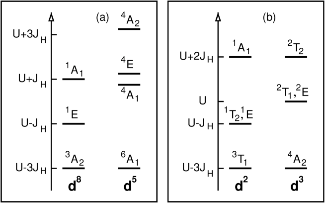
Fig. 5: Energies of charge excitations $\varepsilon_{n}$ (35) for selected cubic transition metal oxides, for: (a) $e_{g}$ excitations to Cu³⁺ ($d^{8}$) and Mn²⁺ ($d^{5}$) ions; (b) $t_{2g}$ excitations to Ti²⁺ ($d^{2}$) and V²⁺ ($d^{3}$) ions. The splittings between different states are due to Hund’s exchange element $J_{H}$ which refers to a pair of $e_{g}$ and $t_{2g}$ electrons in (a) and (b). Image is reproduced from Ref. [8].

Effective interactions in a Mott (or charge transfer) insulator with orbital degeneracy take the form of spin-orbital superexchange [4, 18]. Its general structure is given by the sum over all the nearest neighbor bonds $\langle ij\rangle\!\parallel\!\gamma$ connecting two transition metal ions and over the excitations $n$ possible for each of them as,

$${\cal H}=-\sum_{n}\frac{t^{2}}{\varepsilon_{n}}\sum_{\langle ij\rangle\parallel\gamma}\,P_{\langle ij\rangle}({\cal S})\,{\cal O}_{\langle ij\rangle}^{\gamma},$$ (36)

where $P_{\langle ij\rangle}({\cal S})$ is the projection on the total spin ${\cal S}=S\pm\frac{1}{2}$ and ${\cal O}_{\langle ij\rangle}^{\gamma}$ is the projection operator on the orbital state at the sites $i$ and $j$ of the bond. Following this general procedure, one finds a spin-orbital model with Heisenberg spin interaction for spins $S=\frac{m}{2}$ of SU(2) symmetry coupled to the orbital operators which have much lower cubic symmetry, with the general structure of spin-orbital superexchange $\propto J$ (1) [8],

$${\cal H}_{J}=J\sum_{\gamma}\sum_{\langle ij\rangle\parallel\gamma}\left\{{\hat{\cal K}}_{ij}^{(\gamma)}\left({\vec{S}}_{i}\cdot{\vec{S}}_{j}+S^{2}\right)+{\hat{\cal N}}_{ij}^{(\gamma)}\right\}.$$ (37)

It connects ions at sites $i$ and $j$ along the bond $\langle ij\rangle\parallel\gamma$ and involves orbital operators, ${\hat{\cal K}}_{ij}^{(\gamma)}$ and ${\hat{\cal N}}_{ij}^{(\gamma)}$ which depend on the bond direction $\gamma=a,b,c$ for the three a priori equivalent directions in a cubic crystal. The spin scalar product, $\left({\vec{S}}_{i}\cdot{\vec{S}}_{j}\right)$, is coupled to orbital operators ${\hat{\cal K}}_{ij}^{(\gamma)}$ which together with the other ”decoupled” orbital operators, ${\hat{\cal N}}_{ij}^{(\gamma)}$, determine the orbital state in a Mott insulator. The form of these operators depends on the type of orbital degrees of freedom in a given model. They involve active orbitals on each bond $\langle ij\rangle\parallel\gamma$ along direction $\gamma$. Thus the orbital interactions are directional and have only the cubic symmetry of a (perovskite) lattice provided the symmetry in the orbital sector is not broken by other interactions, for instance by crystal-field or Jahn-Teller terms.

The magnetic superexchange constants along each cubic axis $J_{ab}$ and $J_{c}$ in the effective spin model,

$$H=J_{ab}\sum_{\langle ij\rangle\parallel ab}{\vec{S}}_{i}\cdot{\vec{S}}_{j}+J_{c}\sum_{\langle ij\rangle\parallel c}{\vec{S}}_{i}\cdot{\vec{S}}_{j},$$ (38)

are obtained from the spin-orbital model (37) by decoupling spin and orbital operators and next averaging the orbital operators over a given orbital (ordered or disordered) state. It gives effective magnetic exchange interactions: $J_{c}$ along the $c$ axis, and $J_{ab}$ within the $ab$ planes. The latter $J_{ab}$ ones could in principle still be different between the $a$ and $b$ axes in case of finite lattice distortions due to the Jahn-Teller effect or octahedra tilting, but we limit ourselves to idealized structures with $J_{ab}$ being the same for both planar directions. We show below that the spin-spin correlations along the $c$ axis and within the $ab$ planes,

$$s_{c}=\langle\vec{S}_{i}\cdot\vec{S}_{j}\rangle_{c},\hskip 19.91684pts_{ab}=\langle\vec{S}_{i}\cdot\vec{S}_{j}\rangle_{ab},$$ (39)

next to the orbital correlations, play an important role in the intensity distribution in optical spectroscopy.

In the correlated insulators with partly occupied degenerate orbitals not only the structure of the superexchange (37) is complex, but also the optical spectra exhibit strong anisotropy and temperature dependence near the magnetic transitions, as found e.g. in LaMnO₃ [28] or in the cubic vanadates LaVO₃ and YVO₃ [29]. In such systems several excitations contribute to the excitation spectra, so one may ask how the spectral weight redistributes between individual subbands originating from these excitations. The spectral weight distribution is in general anisotropic already when orbital order sets in and breaks the cubic symmetry, but even more so when $A$-type or $C$-type AF spin order occurs below the Néel temperature $T_{\rm N}$.

At orbital degeneracy the superexchange consists of the terms $H_{n}^{(\gamma)}(ij)$ as a superposition of individual contributions on each bond $\langle ij\rangle$ due to charge excitation $n$ (35) [19],

$${\cal H}=J\sum_{n}\sum_{\langle ij\rangle\parallel\gamma}H_{n}^{(\gamma)}(ij),$$ (40)

with the energy unit for each individual $H_{n}^{(\gamma)}(ij)$ term given by the superexchange constant $J$ (1). It follows from $d-d$ charge excitations with an effective hopping element $t$ between neighboring transition metal ions and is the same as that obtained in a Mott insulator with nondegenerate orbitals in the regime of $U\gg t$. The spectral weight in the optical spectroscopy is determined by the kinetic energy, and reflects the onset of magnetic order and/or orbital order [19]. In a correlated insulator the electrons are almost localized and the only kinetic energy which is left is associated with the same virtual charge excitations that contribute also to the superexchange. Therefore, the individual kinetic energy terms $K_{n}^{(\gamma)}$ may be directly determined from the superexchange (40) using the Hellman-Feynman theorem,

$$K_{n}^{(\gamma)}=-2J\left\langle H_{n}^{(\gamma)}(ij)\right\rangle.$$ (41)

For convenience, we define here the $K_{n}^{(\gamma)}$ as positive quantities. Each term $K_{n}^{(\gamma)}$ (41) originates from a given charge excitation $n$ along a bond $\langle ij\rangle\parallel\gamma$. These terms are directly related to the partial optical sum rule for individual Hubbard subbands, which reads [19]

$$\frac{a_{0}\hbar^{2}}{e^{2}}\int_{0}^{\infty}\sigma_{n}^{(\gamma)}(\omega)d\omega=\frac{\pi}{2}K_{n}^{(\gamma)},$$ (42)

where $\sigma_{n}^{(\gamma)}(\omega)$ is the contribution of band $n$ to the optical conductivity for polarization along the $\gamma$ axis, $a_{0}$ is the distance between transition metal ions, and the tight-binding model with nearest neighbor hopping is implied. Using Eq. (41) one finds that the intensity of each band is indeed determined by the underlying orbital order together with the spin-spin correlation along the direction corresponding to the polarization.

One has to distinguish the above partial sum rule (42) from the full sum rule for the total spectral weight in the optical spectroscopy for polarization along a cubic direction $\gamma$, involving

$$K^{(\gamma)}=-2J\sum_{n}\big{\langle}H_{n}^{(\gamma)}(ij)\big{\rangle},$$ (43)

which stands for the total intensity in the optical $d-d$ excitations. This quantity is usually of less interest as it does not allow for a direct insight into the nature of the electronic structure being a sum over several excitations with different energies $\varepsilon_{n}$ (35) and has a much weaker temperature dependence. In addition, it might be also more difficult to deduce from experiment.

3.2 Kugel-Khomskii model for KCuF₃ and K₂CuF₄

The simplest and seminal spin-orbital model is obtained when a fermion has two flavors, spin and orbital, and both have two components, i.e., spin and pseudospin are $S=T=\frac{1}{2}$. The physical realization is found in cuprates with degenerate $e_{g}$ orbitals, such as KCuF₃ or K₂CuF₄ [4], where Cu²⁺ ions are in the $d^{9}$ electronic configuration, so charge excitations $d_{i}^{9}d_{j}^{9}\rightleftharpoons d_{i}^{10}d_{j}^{8}$ are made by holes. By considering the degenerate Hubbard model for two $e_{g}$ orbitals one finds that $d^{8}$ ions have an equidistant multiplet structure, with three excitation energies which differ by $2J_{H}$ [here $J_{H}$ stands for $J_{H}^{e}$ in Eq. (16)], see Table 2. We emphasize that the correct spectrum has a doubly degenerate energy $(U-J_{H})$ and the highest non-degenerate energy is $(U+J_{H})$, see Fig. 5(a). Note that this result follows from the diagonalization of the local Coulomb interactions in the relevant subspaces — it reflects the fact that a double occupancy ($|z{\uparrow}z{\downarrow}\rangle$ or $|\bar{z}{\uparrow}\bar{z}{\downarrow}\rangle$) in either orbital state ($|z\rangle$ or $|\bar{z}\rangle$) is not an eigenstate of the degenerate Hubbard in the atomic limit (17), so the excitation energy $U$ is absent in the spectrum, see Table 2.

Table 2: Elements needed for the construction of the Kugel-Khomskii model from charge excitations on the bond $\langle ij\rangle$: excitation $n$, its type (HS or LS) and energy $\varepsilon_{n}$, total spin state (triplet or singlet) and the spin projection operator $P_{\langle ij\rangle}({\cal S})$, and the orbital state and the corresponding orbital projection operator.

charge excitation			spin state		orbital state
$n$	type	$\varepsilon_{n}$	${\cal S}$	$P_{\langle ij\rangle}({\cal S})$	orbitals on $\langle ij\rangle\parallel\gamma$	projection
1	HS	$U-3J_{H}$	$1$	$\,\,\,\,\left({\vec{S}}_{i}\cdot{\vec{S}}_{j}+\frac{3}{4}\right)$	$|i\zeta_{\gamma}\rangle\,|j\xi_{\gamma}\rangle$ $\left(|i\xi_{\gamma}\rangle\,|j\zeta_{\gamma}\rangle\right)$	${\cal P}_{\langle ij\rangle}^{(\gamma)}$
2	LS	$U-J_{H}$	$0$	$-\left({\vec{S}}_{i}\cdot{\vec{S}}_{j}-\frac{1}{4}\right)$	$|i\zeta_{\gamma}\rangle\,|j\xi_{\gamma}\rangle$ $\left(|i\xi_{\gamma}\rangle\,|j\zeta_{\gamma}\rangle\right)$	${\cal P}_{\langle ij\rangle}^{(\gamma)}$
3	LS	$U-J_{H}$	$0$	$-\left({\vec{S}}_{i}\cdot{\vec{S}}_{j}-\frac{1}{4}\right)$	$|i\zeta_{\gamma}\rangle\,|j\zeta_{\gamma}\rangle$	${\cal Q}_{\langle ij\rangle}^{(\gamma)}$
4	LS	$U+J_{H}$	$0$	$-\left({\vec{S}}_{i}\cdot{\vec{S}}_{j}-\frac{1}{4}\right)$	$|i\zeta_{\gamma}\rangle\,|j\zeta_{\gamma}\rangle$	${\cal Q}_{\langle ij\rangle}^{(\gamma)}$

The total spin state on the bond corresponds to ${\cal S}=1$ or 0, so the spin projection operators $P_{\langle ij\rangle}(1)$ and $P_{\langle ij\rangle}(0)$ are easily deduced, see Table 2. The orbital configuration which corresponds to a given bond $\langle ij\rangle$ is given by one of the orbital operators in Sec. 2, either ${\cal P}_{\langle ij\rangle}^{(\gamma)}$ for the doubly occupied states involving different orbitals, or ${\cal Q}_{\langle ij\rangle}^{(\gamma)}$ for a double occupancy in a directional orbital at site $i$ or $j$. This gives a rather transparent structure of one HS and three LS excitations in Table 2. The 3D Kugel-Khomskii (KK) model then follows from Eq. (36) [20, 21]:

$${\cal H}(d^{9}) = \sum_{\gamma}\sum_{\langle ij\rangle\parallel\gamma}\left\{-\frac{t^{2}}{U-3J_{H}}\left({\vec{S}}_{i}\cdot{\vec{S}}_{j}+\frac{3}{4}\right){\cal P}_{\langle ij\rangle}^{(\gamma)}+\frac{t^{2}}{U-J_{H}}\left({\vec{S}}_{i}\cdot{\vec{S}}_{j}-\frac{1}{4}\right){\cal P}_{\langle ij\rangle}^{(\gamma)}\right.$$ (44)

$$\hskip 51.21504pt\left.+\left(\frac{t^{2}}{U-J_{H}}+\frac{t^{2}}{U+J_{H}}\right)\left({\vec{S}}_{i}\cdot{\vec{S}}_{j}-\frac{1}{4}\right){\cal Q}_{\langle ij\rangle}^{(\gamma)}\right\}+E_{z}\sum_{i}\tau_{i}^{c}.$$

The last term $\propto E_{z}$ is the crystal field which splits off the degenerate $e_{g}$ orbitals when Jahn-Teller lattice distortion occurs, and is together with Hund’s exchange $\eta$ a second parameter to construct phase diagrams, see below. Here it refers to holes, i.e., large $E_{z}>0$ favors hole occupation in $|\bar{z}\rangle\equiv|x^{2}-y^{2}\rangle/\sqrt{2}$ orbitals, as in La₂CuO₄. On the other hand, while $E_{z}\simeq 0$, both orbitals have almost equal hole density.

Another form of the Hamiltonian (44) is obtained by introducing the coefficients,

$$r_{1}=\frac{1}{1-3\eta},\hskip 19.91684ptr_{2}=r_{3}=\frac{1}{1-\eta},\hskip 19.91684ptr_{4}=\frac{1}{1+\eta},$$ (45)

and defining the superexchange constant $J$ in the same way as in the $t-J$ model Eq. (1). With the explicit representation of the orbital operators ${\cal P}_{\langle ij\rangle}^{(\gamma)}$ and ${\cal Q}_{\langle ij\rangle}^{(\gamma)}$ in terms of $\left\{\tau_{i}^{(\gamma)}\right\}$ one finds,

$${\cal H}(d^{9})\!\! = \!\frac{1}{2}J\sum_{\gamma}\sum_{\langle ij\rangle\parallel\gamma}\left\{\left[-r_{1}\left({\vec{S}}_{i}\cdot{\vec{S}}_{j}+\frac{3}{4}\right)+r_{2}\left({\vec{S}}_{i}\cdot{\vec{S}}_{j}-\frac{1}{4}\right)\right]\left(\frac{1}{4}-\tau_{i}^{(\gamma)}\tau_{j}^{(\gamma)}\right)\right.$$ (46)

$$\!\hskip 19.91684pt\left.+\left(r_{3}+r_{4}\right)\left({\vec{S}}_{i}\cdot{\vec{S}}_{j}-\frac{1}{4}\right)\left(\tau_{i}^{(\gamma)}+\frac{1}{2}\right)\left(\tau_{j}^{(\gamma)}+\frac{1}{2}\right)\right\}+E_{z}\sum_{i}\tau_{i}^{c}.$$

In the FM state spins are integrated out and one finds from the first term just the superexchange in the $e_{g}$ orbital model analyzed before in Sec. 2.

The magnetic superexchange constants $J_{ab}$ and $J_{c}$ in the effective spin-orbital model (46) are obtained by decoupling spin and orbital operators and next averaging the orbital operators $\left\langle{\hat{\cal K}}_{ij}^{(\gamma)}\right\rangle$ over the classical state $|\Phi_{0}\rangle$ as given by Eq. (29). The relevant averages are given in Table 3, and they lead to the following expressions for the superexchange constants in Eq. (38),

$$J_{c} = \frac{1}{8}J\Big{\{}-r_{1}\sin^{2}\theta+(r_{2}+r_{3})(1+\cos\theta)+r_{4}(1+\cos\theta)^{2}\Big{\}},$$ (47)

$$J_{ab} = \frac{1}{8}J\left\{-r_{1}\left(\frac{3}{4}+\sin^{2}\theta\right)+(r_{2}+r_{3})\left(1-\frac{1}{2}\cos\theta\right)+r_{4}\left(\frac{1}{2}-\cos\theta\right)^{2}\right\},$$ (48)

which depend on two parameters: $J$ (1) and $\eta$ (26), and on the orbital order (2) specified by the orbital angle $\theta$. It is clear that the FM term $\propto r_{1}$ competes with all the other AF LS terms. Nevertheless, in the $ab$ planes, where the occupied hole $e_{g}$ orbitals alternate, the larger FM contribution dominates and makes the magnetic superexchange $J_{ab}$ weakly FM ($J_{ab}\lesssim 0$) (when $\sin^{2}\theta\simeq 1$), while the stronger AF superexchange along the $c$ axis ($J_{c}\gg|J_{ab}|$) favors quasi one-dimensional (1D) spin fluctuations. Thus KCuF₃ exhibits spinon excitations for $T>T{\rm N}$.

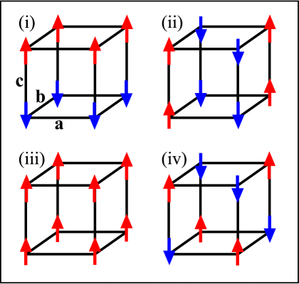
Fig. 6: Left — schematic view of four simplest orbital configurations on a representative cube of the 3D lattice: (a) AO order with $\langle\tau_{i}^{a(b)}\rangle=\pm\frac{1}{2}$ changing from site to site and $\langle\tau_{i}^{c}\rangle=\frac{1}{4}$, obtained for $E_{z}<0$, (b) AO order with $\langle\tau_{i}^{a(b)}\rangle=-\frac{1}{2}$ changing from site to site and $\langle\tau_{i}^{c}\rangle=-\frac{1}{4}$, obtained for $E_{z}>0$, (c) FO order with occupied $z$ orbitals and $\langle\tau_{i}^{c}\rangle=\frac{1}{2}$ (cigar-shaped orbitals), and (d) FO order with occupied $\bar{z}$ orbitals and $\langle\tau_{i}^{c}\rangle=-\frac{1}{2}$ (clover-shaped orbitals). Right — schematic view of four spin configurations (arrows stand for up or down spins) in phases with spin order: (i) $A$-AF, (ii) $C$-AF, (iii) FM, and (iv) $G$-AF. Images are reproduced from Ref. [24].

Table 3: Averages of the orbital projection operators standing in the spin-orbital interactions in the KK model (46) and determine the spin interactions in $H_{s}$ (38) for the $C$-type orbital order of occupied $e_{g}$ orbitals which alternate in $ab$ planes, as given by Eqs. (2). Nonequivalent cubic directions are labeled by $\gamma=ab,c$.

operator	average		$ab$		$c$
${\cal Q}_{\langle ij\rangle}^{(\gamma)}$	$2\left\langle\big{(}\frac{1}{2}-\tau_{i}^{(\gamma)}\big{)}\big{(}\frac{1}{2}-\tau_{j}^{(\gamma)}\big{)}\right\rangle$		$\frac{1}{2}\big{(}\frac{1}{2}-\cos\theta\big{)}^{2}$		$\frac{1}{2}\big{(}1+\cos\theta\big{)}^{2}$
${\cal P}_{\langle ij\rangle}^{(\gamma)}$	$\left\langle\frac{1}{4}-\tau_{i}^{(\gamma)}\tau_{j}^{(\gamma)}\right\rangle$		$\frac{1}{4}\big{(}\frac{3}{4}+\sin^{2}\theta\big{)}$		$\frac{1}{4}\sin^{2}\theta$
${\cal R}_{\langle ij\rangle}^{(\gamma)}$	$2\left\langle\big{(}\frac{1}{2}+\tau_{i}^{(\gamma)}\big{)}\big{(}\frac{1}{2}+\tau_{j}^{(\gamma)}\big{)}\right\rangle$		$\frac{1}{2}\big{(}\frac{1}{2}+\cos\theta\big{)}^{2}$		$\frac{1}{2}\big{(}1-\cos\theta\big{)}^{2}$

Consider first the 2D KK model on a square lattice, with $\gamma=a,b$ in Eq. (46), as in K₂CuF₄. In the absence of Hund’s exchange, interactions between $S=\frac{1}{2}$ spins are AF. However, they are quite different depending on which of the two $e_{g}$ orbitals are occupied by holes: $J_{ab}^{z}=\frac{1}{16}J$ for $|z\rangle$ and $J_{ab}^{\bar{z}}=\frac{9}{16}J$ for $|\bar{z}\rangle$ hole orbitals. As a result, the AF phases with spin order in Fig. 6(iv) and the FO order shown in Figs. 6(c) and 6(d) are degenerate at finite crystal field $E_{z}=-\frac{1}{2}J$. This defines a quantum critical point $Q_{2{\rm D}}=(-0.5,0)$ in the $(E_{z}/J,\eta)$ plane. Actually, at this point also one more phase has the same energy — the FM spin phase of Fig. 6(i) with AO order of $|\pm\rangle$ orbitals (28) shown in Fig. 6(a) [21].

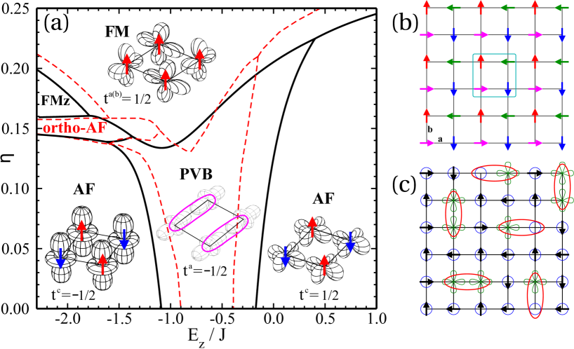
Fig. 7: Spin-orbital phase diagram and entanglement in the 2D KK model: (a) phase diagram in the plaquette mean field (solid lines) and ERA (dashed lines) variational approximation, with insets showing representative spin and orbital configurations on a $2\times 2$ plaquette — ${\bar{z}}$-like $\left(t^{c}\!=\!-\left\langle\tau^{c}_{i}\right\rangle=\frac{1}{2}\right)$ and $z$-like $\left(t^{a,c}\!=\!-\left\langle\tau^{c(a)}_{i}\right\rangle=-\frac{1}{2}\right)$ orbitals are accompanied either by AF long range order (arrows) or by spin singlets on bonds in the PVB phase; (b) view of an exotic four-sublattice ortho-AF phase near the onset of FM (or FM$z$) phase; (c) artist’s view of the ortho-AF phase — spin singlets (ovals) are entangled with either one or two orbital excitations $|z\rangle\rightarrow|\bar{z}\rangle$ (clovers). Images are reproduced from Ref. [22].

To capture the corrections due to quantum fluctuations, one may construct a plaquette mean field approximation or entanglement renormalization ansatz (ERA) [22]. One finds important corrections to a mean field phase diagram near the quantum critical point $Q_{2{\rm D}}$, and a plaquette valence bond (PVB) state is stable in between the above three phases with long range order, with spin singlets on the bonds $\parallel\!a$ $\left(\parallel\!b\right)$, stabilized by the directional orbitals $|\zeta_{a}\rangle$ $\left(|\zeta_{b}\rangle\right)$. A novel ortho-AF phase appears as well when the magnetic interactions change from AF to FM ones due to increasing Hund’s exchange $\eta$, and for $E_{z}/J<-1.5$, see Fig. 7(a). Since the nearest neighbor magnetic interactions are very weak, exotic four-sublattice ortho-AF spin order is stabilized by second and third nearest neighbor interactions, shown in Fig. 7(b). Such further neighbor interactions follow from spin-orbital excitations shown in Fig. 7(c). Note that both approximate methods employed in Ref. [22] (plaquette mean field approximation and ERA) give very similar range of stability of ortho-AF phase.

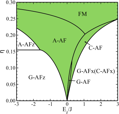
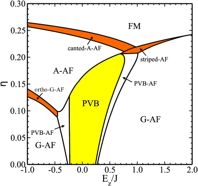
(a)     (b)

Fig. 8: Phase diagram of the 3D KK model obtained in two mean field methods: (a) the single-site mean field, and (b) the cluster mean field. Shaded (green) area indicates phases with AO order while the remaining magnetic phases are accompanied by FO order with fully polarized orbitals, either ${\bar{z}}$ ($x$) (for $E_{z}>0$) or $z$ (for $E_{z}<0$). In this approach plaquette valence-bond (PVB) phase with alternating spin singlets in the $ab$ planes (yellow) separates the phases with magnetic long range order, see Fig. 6. Phases with exotic magnetic order are shown in orange. Note different ranges of $E_{z}/J$ shown. Images are reproduced from Ref. [24].

In the 3D KK model the exchange interaction in the $ab$ planes (48) and along the $c$ axis (47) are exactly balanced at the orbital degeneracy ($E_{z}=0$) and the quantum critical point where several classical phases meet in mean field approximation is $Q_{3{\rm D}}=(0,0)$, see Fig. 8(a). While finite $E_{z}$ favors one or the other $G$-AF phase, finite Hund’s exchange $\eta$ favors AO order stabilizing $A$-AF spin order, see Fig. 6(i). This phase is indeed found in KCuF₃ at low temperature $T<T_{\rm N}$ and is also obtained from the electronic structure calculations [23]. We remark that for unrealistically large $\eta>0.2$, spin order changes to FM.

Large qualitative changes in the phase diagram are found when spin correlations on bonds are treated in cluster mean field approximation (using plaquettes or linear clusters [24]), see Fig. 8(b). Phases with long range spin order ($G$-AF, $A$-AF, and FM) are again separated by exotic types of magnetic order which arise by a similar mechanism to that described above for an $ab$ monolayer, i.e., nearest neighbor exchange changes sign along one cubic direction. Near the QCP $Q_{3{\rm D}}$ one finds again PVB phase, as in the 2D KK model. In addition to the phase diagram of Fig. 7(a), the transitions between $G$-AF and PVB phases are continuous and mixed PVB-AF phases arise.

3.3 Spin-orbital superexchange model for LaMnO₃

Electronic structure calculations give $A$-AF spin order, in agreement with experiment. It follows from the spin-orbital superexchange for spins $S=2$ in LaMnO₃, ${\cal H}_{e}$, due to the excitations involving $e_{g}$ electrons. The energies of the five possible excited states [9] shown in Fig. 5(a) are: ($i$) the HS (${\cal S}=\frac{5}{2}$) ${}^{6}\!A_{1}$ state, and ($ii$) the LS (${\cal S}=\frac{3}{2}$) states: ${}^{4}\!A_{1}$, ${}^{4}E$ (${}^{4}E_{\epsilon}$, ${}^{4}E_{\theta}$), and ${}^{4}\!A_{2}$, will be parameterized again by the intraorbital Coulomb element $U$ and by Hund’s exchange $J_{H}^{e}$ between a pair of $e_{g}$ electrons in a Mn²⁺ ($d^{5}$) ion, defined in Eq. (16). The Racah parameters $B=0.107$ eV and $C=0.477$ eV justify an approximate relation $C\simeq 4B$, and we find the LS excitation spectrum: $\varepsilon(^{4}\!A_{1})=U+\frac{3}{4}J_{H}$, $\varepsilon(^{4}E)=U+\frac{5}{4}J_{H}$ (twice), and $\varepsilon(^{4}\!A_{2})=U+\frac{13}{4}J_{H}$.

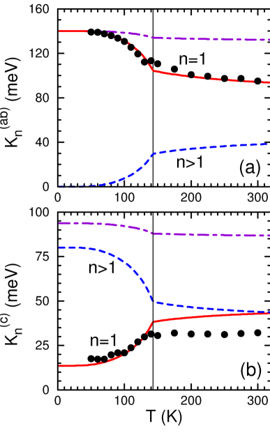
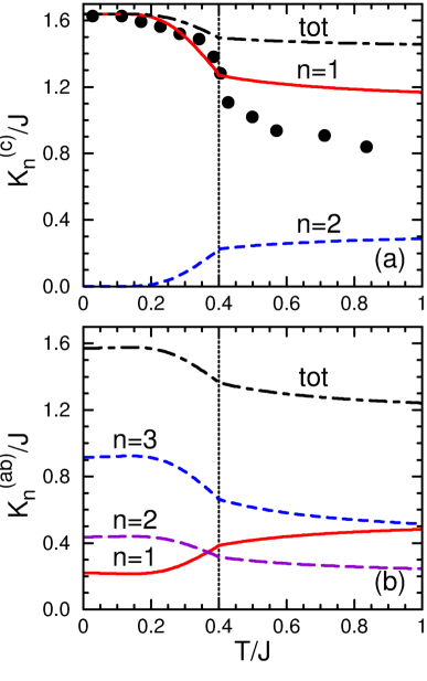
(A)       (B)

Fig. 9: Kinetic energies per bond $K_{n}^{(\gamma)}$ (41) for increasing temperature $T$ obtained from the respective spin-orbital models for FM (top) and AF (bottom) bonds along the axis $\gamma$: (A) LaMnO₃ (with $J=150$ meV, $\eta\simeq 0.18$ [8], end experimental points [28]); (B) LaVO₃ with $\eta\!=\!0.13$ [19] and experimental points [29]. The kinetic energies in HS states ($n=1$, red lines) and compared with the experiment (filled circles). Vertical dotted lines indicate the value of $T_{N}$. Images are reproduced from Ref. [8].

Using the spin algebra (Clebsch-Gordan coefficients) and considering again two possible $e_{g}$ orbital configurations, see Eqs. (22) and (23), and charge excitations by $t_{2g}$ electrons, one finds a compact expression [25],

$${\cal H}_{e}\!\! = \!\!\frac{1}{16}\sum_{\gamma}\!\sum_{\langle ij\rangle\parallel\gamma}\left\{-\frac{8}{5}\frac{t^{2}}{\varepsilon(^{6}A_{1})}\left(\vec{S}_{i}\cdot\vec{S}_{j}+6\right){\cal P}_{\langle ij\rangle}^{(\gamma)}+\left[\frac{t^{2}}{\varepsilon(^{4}E)}+\frac{3}{5}\frac{t^{2}}{\varepsilon(^{4}A_{1})}\right]\left(\vec{S}_{i}\cdot\vec{S}_{j}-4\right){\cal P}_{\langle ij\rangle}^{(\gamma)}\right.$$ (49)

$$\left.\hskip 62.59596pt+\left[\frac{t^{2}}{\varepsilon(^{4}E)}+\frac{t^{2}}{\varepsilon(^{4}A_{2})}\right]\left(\vec{S}_{i}\cdot\vec{S}_{j}-4\right){\cal Q}_{\langle ij\rangle}^{(\gamma)}\right\}+E_{z}\sum_{i}\tau_{i}^{c}.$$

$${\cal H}_{t}\!\! = \frac{1}{8}J\beta r_{t}\Big{(}\vec{S}_{i}\!\cdot\!\vec{S}_{j}-4\Big{)}.$$ (50)

Here $\beta=(t_{\pi}/t)^{2}$ follows from the difference between the effective $d-d$ hopping elements along the $\sigma$ and $\pi$ bonds, i.e., $\beta\simeq\frac{1}{9}$, while the coefficient $r_{t}$ stands for a superposition of all $t_{2g}$ excitations involved in the $t_{2g}$ superexchange [8]. Note that spin-projection operators for high (low) total spin ${\cal S}=2$ (${\cal S}=1$) cannot be used, but again the HS term stands for a FM contribution which dominates over the other LS terms when $\left\langle{\cal P}_{\langle ij\rangle}^{(\gamma)}\right\rangle\simeq 1$. Charge excitations by $t_{2g}$ electrons give double occupancies in active $t_{2g}$ orbitals, so ${\cal H}_{t}$ is AF but this term is small — as a result FM interactions may dominate but again only along two spatial directions. Indeed, this happens for the realistic parameters of LaMnO₃ for the $ab$ planes where spin order is FM and coexists with AO order, while along the $c$ axis spin order is AF accompanied by FO order, i.e., spin-orbital order is $A$-AF/$C$-AF. Indeed, this type of order is found both from the theory for realistic parameters and from the electronic structure calculations [26]. One concludes that Jahn-Teller orbital interactions are responsible for the enhanced value of the orbital transition temperature [27].

The optical spectral weight due to HS states in LaMnO₃ may be easily derived from the present model (49), following the general theory, see Eq. (41). One finds a very satisfactory agreement between the present theory and the experimental results of [28], as shown in Fig. 9(A). We emphasize, that no fit is made here, i.e., the kinetic energies (41) are calculated using the same parameters as those used for the magnetic exchange constants [8]. Therefore, such a good agreement with experiment suggests that indeed the spin-orbital superexchange may be disentangled, as also verified later [27].

(a)      (b)

Fig. 10: Band structure along the high symmetry directions in: (a) $G$-AF phase at $x=0$ and (b) $C$-AF phase at $x=0.05$. Spin majority (minority) bands are shown by solid (dashed) lines. Parameters: $t=0.4$ eV, $J_{H}=0.74$ eV, $g=3$ eV. Insets shows the Fermi surfaces at low doping. The special points: $\Gamma=(0,0,0)$, $X=(\pi,0,0)$, $M=(\pi,\pi,0)$, $R=(\pi,\pi,\pi)$, $Z=(0,0,\pi)$. Images are reproduced from Ref. [30].

To give an example of a phase transition triggered by $e_{g}$ electron doping of Sr_1-xLa_xMnO₃ we show the results obtained with double exchange model for degenerate $e_{g}$ electrons extended by the coupling to the lattice [30],

$${\cal H}\!=-\!\sum_{ij,\alpha\beta,\sigma}t_{\alpha\beta}^{ij}a_{i\alpha\sigma}^{\dagger}a_{j\beta\sigma}-2J_{H}\sum_{i}{\vec{S}}_{i}\cdot{\vec{s}}_{i}+\!J\sum_{\langle ij\rangle}{\vec{S}}_{i}\cdot{\vec{S}}_{j}-\!gu\sum_{i}(n_{iz}-n_{i\bar{z}})+\!\frac{1}{2}NKu^{2}.$$ (51)

It includes the hopping of $e_{g}$ electrons between orbitals $\alpha=z,\bar{z}$ as in Eq. (6). The tetragonal distortion $u$ is finite only in the $C$-AF phase. Here we define it as proportional to a difference between two lattice constants $a$ and $c$ along the respective axis, $u\equiv 2(c-a)/(c+a)$, and $N$ is the number of lattice sites. The microscopic model that explains the mechanism of the magnetic transition in electron doped manganites from canted $G$-AF to collinear $C$-AF phase at low doping $x\simeq 0.04$. The double exchange supported by the cooperative Jahn-Teller effect leads then to dimensional reduction from an isotropic 3D $G$-AF phase to a quasi-1D order of partly occupied $3z^{2}-r^{2}$ orbitals in the $C$-AF phase [30]. We emphasize that this theory prediction relies on the shape of the Fermi surface which is radically different in the $G$-AF and $C$-AF phase. Due to the Fermi surface topology, spin canting is suppressed in the $C$-AF phase, in agreement with the experiment.

4 Superexchange for active $t_{2g}$ orbitals

4.1 Spin-orbital superexchange model for LaTiO₃

LaTiO₃ would be electron-hole symmetric compound to KCuF₃, if not the orbital degree of freedom which $t_{2g}$ here. This changes the nature of orbital operators from the projections for each bond to scalar products of pseudospin $T=\frac{1}{2}$ operators. The superexchange spin-orbital model (37) in the perovskite titanates couples $S=\frac{1}{2}$ spins and $T=\frac{1}{2}$ pseudospins arising from the $t_{2g}$ orbital degrees of freedom at nearest neighbor Ti³⁺ ions, e.g. in LaTiO₃ or YTiO₃ [6]. Due to large intraorbital Coulomb element $U$ electrons localize and the densities satisfy the local constraint at each site $i$,

$$n_{ia}+n_{ib}+n_{ic}=1.$$ (52)

The charge excitations lead to one of four different excited states [9], shown in Fig. 5(b): ($i$) the high-spin ${}^{3}T_{1}$ state at energy $U-3J_{H}$, and ($ii$) three low-spin states — degenerate ${}^{1}T_{2}$ and ${}^{1}E$ states at energy $(U-J_{H})$, and ($iii$) an ${}^{1}\!A_{1}$ state at energy $(U+2J_{H})$. As before, the excitation energies are parameterized by $\eta$, defined by Eq. (26), and we introduce the coefficients

$$r_{1}=\frac{1}{1-3\eta},\hskip 19.91684ptr_{2}=\frac{1}{1-\eta},\hskip 19.91684ptr_{3}=\frac{1}{1+2\eta}.$$ (53)

One finds the following compact expressions for the terms contributing to superexchange ${\cal H}_{J}(d^{1})$ Eq. (40) [6]:

$$H_{1}^{(\gamma)}\! = \!\frac{1}{2}Jr_{1}\left(\vec{S}_{i}\!\cdot\!\vec{S}_{j}+\frac{3}{4}\right)\left(A_{ij}^{(\gamma)}\!-\frac{1}{2}n_{ij}^{(\gamma)}\right),$$ (54)

$$H_{2}^{(\gamma)}\! = \!\frac{1}{2}Jr_{2}\left(\vec{S}_{i}\!\cdot\!\vec{S}_{j}-\frac{1}{4}\right)\left(A_{ij}^{(\gamma)}\!-\frac{2}{3}B_{ij}^{(\gamma)}\!+\frac{1}{2}n_{ij}^{(\gamma)}\right),$$ (55)

$$H_{3}^{(\gamma)}\! = \!\frac{1}{3}Jr_{3}\left(\vec{S}_{i}\!\cdot\!\vec{S}_{j}-\frac{1}{4}\right)B_{ij}^{(\gamma)},$$ (56)

where

$$A_{ij}^{(\gamma)}\!=2\left(\vec{\tau}_{i}\cdot\vec{\tau}_{j}+\frac{1}{4}n_{i}n_{j}\right)^{(\gamma)}\!,\hskip 8.5359ptB_{ij}^{(\gamma)}\!=2\left(\vec{\tau}_{i}\otimes\vec{\tau}_{j}+\frac{1}{4}n_{i}n_{j}\right)^{(\gamma)}\!,\hskip 8.5359ptn_{ij}^{(\gamma)}\!=n_{i}^{(\gamma)}+n_{j}^{(\gamma)}.$$ (57)

As in Sec. 3.2, the orbital (pseudospin) operators $\left\{A_{ij}^{(\gamma)},B_{ij}^{(\gamma)},n_{ij}^{(\gamma)}\right\}$ depend on the direction of the $\langle ij\rangle\parallel\gamma$ bond. Their form follows from two active $t_{2g}$ orbitals (flavors) along the cubic axis $\gamma$, e.g. for $\gamma=c$ the active orbitals are $a$ and $b$, and they give two components of the pseudospin $T=\frac{1}{2}$ operator $\vec{\tau}_{i}$. The operators $\left\{A_{ij}^{(\gamma)},B_{ij}^{(\gamma)}\right\}$ describe the interactions between these two active orbitals, which include the quantum fluctuations, and take either the form of a scalar product $\vec{\tau}_{i}\cdot\vec{\tau}_{j}$ in $A_{ij}^{(\gamma)}$, or lead to a similar expression,

$$\vec{\tau}_{i}\otimes\vec{\tau}_{j}=\tau_{i}^{x}\tau_{j}^{x}-\tau_{i}^{y}\tau_{j}^{y}+\tau_{i}^{z}\tau_{i}^{z},$$ (58)

in $B_{ij}^{(\gamma)}$. These latter terms enhance orbital fluctuations by double excitations due to the $\tau_{i}^{+}\tau_{j}^{+}$ and $\tau_{i}^{-}\tau_{j}^{-}$ terms. The interactions along the axis $\gamma$ are tuned by the number of electrons occupying active orbitals, $n_{i}^{(\gamma)}=1-n_{i\gamma}$, which is fixed by the number of electrons in the inactive orbital $n_{i\gamma}$ by the constraint (52). The cubic titanates are known to have particularly pronounced quantum spin-orbital fluctuations [18], and their proper treatment requires a rather sophisticated approach. Therefore, in contrast to AF long range order found in $e_{g}$-orbital systems, spin-orbital disordered state may occur in titanium perovskites, as suggested for LaTiO₃ [6].

4.2 Spin-orbital superexchange model for LaVO₃

As the last cubic system we present the spin-orbital model for V³⁺ ions in $d^{2}$ configurations in the vanadium perovskite $R$VO₃ ($R$=La,$\dots$,Lu). Due to Hund’s exchange one has $S=1$ spins and three ($n=1,2,3$) charge excitations $\varepsilon_{n}$ arising from the transitions to [see Fig. 5(b)]: ($i$) a high-spin state ${}^{4}\!A_{2}$ at energy $(U-3J_{H})$, ($ii$) two degenerate low-spin states ${}^{2}T_{1}$ and ${}^{2}E$ at $U$, and ($iii$) ${}^{2}T_{2}$ low-spin state at $(U+2J_{H})$ [31]. Using $\eta$ (26) we parameterize this multiplet structure by

$$r_{1}=\frac{1}{1-3\eta},\hskip 28.45274ptr_{3}=\frac{1}{1+2\eta}.$$ (59)

The cubic symmetry is broken and the crystal field induces orbital splitting in $R$VO₃, hence $\langle n_{ic}\rangle=1$ and the orbital degrees of freedom are given by the doublet $\{a,b\}$ which defines the pseudospin operators ${\vec{\tau}}_{i}$ at site $i$. One derives a HS contribution $H_{1}^{(c)}(ij)$ for a bond ${\langle ij\rangle}$ along the $c$ axis, and $H_{1}^{(ab)}(ij)$ for a bond in the $ab$ plane:

$$H_{1}^{(c)}(ij) = -\frac{1}{3}Jr_{1}\left(\vec{S}_{i}\!\cdot\!\vec{S}_{j}+2\right)\left(\textstyle{\frac{1}{4}}-\vec{\tau}_{i}\!\cdot\!\vec{\tau}_{j}\right),$$ (60)

$$H_{1}^{(ab)}(ij) = -\frac{1}{6}Jr_{1}\left(\vec{S}_{i}\!\cdot\!\vec{S}_{j}+2\right)\left(\textstyle{\frac{1}{4}}-\tau_{i}^{z}\tau_{j}^{z}\right).$$ (61)

In Eq. (60) pseudospin operators $\vec{\tau}_{i}$ describe low-energy dynamics of (initially degenerate) $\{xz,yz\}$ orbital doublet at site $i$; this dynamics is quenched in $H_{1}^{(ab)}$ (61). Here $\frac{1}{3}(\vec{S}_{i}\cdot\vec{S}_{j}+2)$ is the projection operator on the HS state for $S=1$ spins. The terms $H_{n}^{(c)}(ij)$ for LS excitations ($n=2,3$) contain instead the spin operator $(1-\vec{S}_{i}\cdot\vec{S}_{j})$ (which guarantees that these terms cannot contribute for fully polarized spins $\langle\vec{S}_{i}\cdot\vec{S}_{j}\rangle=1$):

$$H_{2}^{(c)}(ij) = -\frac{1}{12}J\left(1-\vec{S}_{i}\!\cdot\!\vec{S}_{j}\right)\left(\textstyle{\frac{7}{4}}-\tau_{i}^{z}\tau_{j}^{z}-\tau_{i}^{x}\tau_{j}^{x}+5\tau_{i}^{y}\tau_{j}^{y}\right),$$

$$H_{3}^{(c)}(ij) = -\frac{1}{4}Jr\left(1-\vec{S}_{i}\!\cdot\!\vec{S}_{j}\right)\left(\textstyle{\frac{1}{4}}+\tau_{i}^{z}\tau_{j}^{z}+\tau_{i}^{x}\tau_{j}^{x}-\tau_{i}^{y}\tau_{j}^{y}\right),$$ (62)

while again the terms $H_{n}^{(ab)}(ij)$ differ from $H_{n}^{(c)}(ij)$ only by orbital operators:

$$H_{2}^{(ab)}(ij) = -\frac{1}{8}J\left(1-\vec{S}_{i}\!\cdot\!\vec{S}_{j}\right)\left(\textstyle{\frac{19}{12}}\mp\textstyle{\frac{1}{2}}\tau_{i}^{z}\mp\textstyle{\frac{1}{2}}\tau_{j}^{z}-\textstyle{\frac{1}{3}}\tau_{i}^{z}\tau_{j}^{z}\right),$$

$$H_{3}^{(ab)}(ij) = -\frac{1}{8}Jr\left(1-\vec{S}_{i}\!\cdot\!\vec{S}_{j}\right)\left(\textstyle{\frac{5}{4}}\mp\textstyle{\frac{1}{2}}\tau_{i}^{z}\mp\textstyle{\frac{1}{2}}\tau_{j}^{z}+\tau_{i}^{z}\tau_{j}^{z}\right),$$ (63)

where upper (lower) sign corresponds to bonds along the $a$($b$) axis.

First we present a mean field approximation for the spin and orbital bond correlations which are determined self-consistently after decoupling them from each other in ${\cal H}_{J}$ (37). Spin interactions in Eq. (38) are given by two exchange constants:

$$J_{c} = \frac{1}{2}J\left\{\eta r_{1}-(r_{1}-\eta r_{1}-\eta r_{3})(\textstyle{\frac{1}{4}}+\langle\vec{\tau}_{i}\!\cdot\!\vec{\tau}_{j}\rangle)-2\eta r_{3}\langle\tau_{i}^{y}\tau_{j}^{y}\rangle\right\},$$

$$J_{ab} = \frac{1}{4}J\left\{1-\eta r_{1}-\eta r_{3}+(r_{1}-\eta r_{1}-\eta r_{3})(\textstyle{\frac{1}{4}}+\langle\tau_{i}^{z}\tau_{j}^{z}\rangle)\right\},$$ (64)

determined by orbital correlations $\langle\vec{\tau}_{i}\!\cdot\!\vec{\tau}_{j}\rangle$ and $\langle\tau_{i}^{\alpha}\tau_{j}^{\alpha}\rangle$. By evaluating them one finds $J_{c}<0$ and $J_{ab}>0$ supporting $C$-AF spin order. In the orbital sector one finds

$$H_{\tau}=\sum_{\langle ij\rangle_{c}}\left[J_{c}^{\tau}\vec{\tau}_{i}\cdot\vec{\tau}_{j}-J(1-s_{c})\eta r_{3}\tau_{i}^{y}\tau_{j}^{y}\right]+J_{ab}^{\tau}\sum_{\langle ij\rangle_{ab}}\tau_{i}^{z}\tau_{j}^{z},$$ (65)

with:

$$J_{c}^{\tau} = \frac{1}{2}J\left[(1+s_{c})r_{1}+(1-s_{c})\eta(r_{1}+r_{3})\right],$$

$$J_{ab}^{\tau} = \frac{1}{4}J\left[(1-s_{ab})r_{1}+(1+s_{ab})\eta(r_{1}+r_{3})\right],$$ (66)

depending on spin correlations: $s_{c}=\langle\vec{S}_{i}\cdot\vec{S}_{j}\rangle_{c}$ and $s_{ab}=-\langle\vec{S}_{i}\cdot\vec{S}_{j}\rangle_{ab}$. In a classical $C$-AF state ($s_{c}=s_{ab}=1$) this mean field procedure becomes exact, and the orbital problem maps to Heisenberg pseudospin chains along the $c$ axis, weakly coupled (as $\eta\ll 1$) along $a$ and $b$ bonds,

$$H_{\tau}^{(0)}=Jr_{1}\left[\sum_{\langle ij\rangle_{c}}\vec{\tau}_{i}\cdot\vec{\tau}_{j}+\frac{1}{2}\eta\left(1+\frac{r_{3}}{r_{1}}\right)\sum_{\langle ij\rangle_{ab}}\tau_{i}^{z}\tau_{j}^{z}\right],$$ (67)

releasing large zero-point energy. Thus, spin $C$-AF and $G$-AO order with quasi-1D orbital quantum fluctuations support each other in $R$VO₃. Orbital fluctuations play here a prominent role and amplify the FM exchange $J_{c}$, making it even stronger that the AF exchange $J_{ab}$ [31].

Having the individual terms $H_{n}^{(\gamma)}$ of the spin-orbital model, one may derive the spectral weights of optical spectra (41). The HS excitations have remarkable temperature dependence and the spectral weight decreases in the vicinity of the magnetic transition at $T_{\rm N}$, see Fig. 9(B). The observed behavior is reproduced in the theory only when spin-orbital interactions are treated in a cluster approach, i.e. they cannot be disentangled, see Sec. 5.2.

(a)     (b)

Fig. 11: Phase transitions in the vanadium perovskites $R$VO₃: (a) phase diagram with the orbital $T_{\rm OO}$ and Néel $T_{N1}$ transition temperature obtained from the theory with and without orbital-lattice coupling (solid and dashed lines) [32], and from experiment (circles) [33]; (b) spin $\langle S_{i}^{z}\rangle$ (solid) and $G$-type orbital $\langle\tau_{i}^{z}\rangle_{G}$ (dashed) order parameters, vanishing at $T_{\rm OO}$ and $T_{N1}$, and the transverse orbital polarization $\langle\tau_{i}^{x}\rangle$ (dashed-dotted lines) for LaVO₃ and SmVO₃ (thin and heavy lines). Images are reproduced from Ref. [32].

Unlike in LaMnO₃ where the spin and orbital phase transitions are well separated, in the $R$VO₃ ($R$=Lu,Yb,$\dots$,La) the two transitions are close to each other [33]. It is not easy to reproduce the observed dependence of the transition temperatures $T_{\rm OO}$ and Néel $T_{N1}$ on the ionic radius $r_{R}$ (in the $R$VO₃ compounds with small $r_{R}$ there is also another magnetic transition at $T_{N2}$ [34] which is not discussed here). The spin-orbital model was extended by the coupling to the lattice to unravel a nontrivial interplay between superexchange, the orbital-lattice coupling due to the GdFeO₃-like rotations of the VO₆ octahedra, and orthorhombic lattice distortions [32]. One finds that the lattice strain affects the onset of the magnetic and orbital order by partial suppression of orbital fluctuations, and the dependence of $T_{\rm OO}$ is non-monotonous in Fig. 11(a). Thereby the orbital polarization $\propto\left\langle\tau^{x}\right\rangle$ increases with decreasing ionic radius $r_{R}$, and the value of $T_{N1}$ is reduced, see Fig. 11(b). The theoretical approach demonstrates that orbital-lattice coupling is very important and reduces both $T_{\rm OO}$ and Néel $T_{N1}$ for small ionic radii.

5 Spin-orbital complementarity and entanglement

5.1 Goodenough-Kanamori rules

While rather advanced many-body treatment of the quantum physics characteristic for spin-orbital models is required in general, we want to present here certain simple principles which help to understand the heart of the problem and to give simple guidelines for interpreting experiments and finding relevant physical parameters of the spin-orbital models of undoped cubic insulators. We will argue that such an approach based upon classical orbital order is well justified in many known cases, as quantum phenomena are often quenched by the Jahn-Teller (JT) coupling between orbitals and the lattice distortions, which are present below structural phase transitions and induce orbital order both in spin-disordered and in spin-ordered or spin-liquid phases.

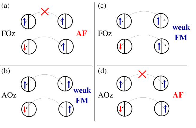
Fig. 12: Artist’s view of the GKR [35] for: (a) FO$z$ and AF spin order and (b) AO$z$ and FM spin order in a system with orbital flavor conserving hopping as is alkali $R$O₂ hyperoxides ($R$=K,Rb,Cs) [36]. The charge excitations generated by interorbital hopping fully violate the GKR and support the states with the same spin-orbital order: (c) FO$z$ and FM spin order and (d) AO$z$ and AF spin order. Image is reproduced from Ref. [36].

From the derivation of the Kugel-Khomskii model in Sec. 3.2, we have seen that pairs of directional orbitals on neighboring ions $\{|i\zeta_{\gamma}\rangle,|j\zeta_{\gamma}\rangle\}$ favor AF spin order while pairs of orthogonal orbitals such as $\{|i\zeta_{\gamma}\rangle,|j\xi_{\gamma}\rangle\}$ favor FM spin order. This is generalized to classical Goodenough-Kanamori rules (GKR) [35] that state that AF spin order is accompanied by FO order, while FM spin order is accompanied by AO order, see Figs. 12(a) and 12(b). Indeed, these rules emphasizing the complementarity of spin-orbital correlations are frequently employed to explain the observed spin-orbital order in several systems, particularly in those where spins are large, like in CMR manganites [3]. They agree with the general structure of spin-orbital superexchange in the Kugel-Khomskii model where it is sufficient to consider the flavor-conserving hopping between pairs of directional orbitals $\{|i\zeta_{\gamma}\rangle,|j\zeta_{\gamma}\rangle\}$. The excited states are then double occupancies in one of the directional orbitals while no effective interaction arises for two parallel spins (in triplet states), so the superexchange is AF. In contrast, for a pair of orthogonal orbitals, e.g. $\{|i\zeta_{\gamma}\rangle,|j\xi_{\gamma}\rangle\}$, two different orbitals are singly occupied and the FM term is stronger than the AF one as the excitation energy is lower. Therefore, configurations with AO order support FM spin order.

The above complementarity of spin-orbital order is frustrated by interorbital hopping, or may be modified by spin-orbital entanglement, see below. In such cases the order in both channels could be the same, either FM/FO, see Fig. 12(c), or AF/AO, see Fig. 12(d). Again, when different orbitals are occupied in the excited state, the spin superexchange is weak FM and when the same orbital is doubly occupied, the spin superexchange is stronger and AF. The latter AF exchange coupling dominates because antiferromagnetism, which is due to the Pauli principle, does not have to compete here with ferromagnetism. On the contrary, FM exchange is caused by the energy difference $\propto\eta$ between triplet and singlet excited states with two different orbitals occupied.

The presented modification of the GKR is of importance in alkali $R$O₂ hyperoxides ($R$=K,Rb,Cs) [36]. The JT effect is crucial for this generalization of the GKR — without it large interorbital hopping orders the $T^{x}$-orbital-mixing pseudospin component instead of the $T^{z}$ component in a single plane. More generally, such generalized GKR can arise whenever the orbital order on a bond is not solely stabilized by the same spin-orbital superexchange interaction that determines the spin exchange. On a geometrically frustrated lattice, another route to this behavior can occur when the ordered orbital component preferred by superexchange depends on the direction and the relative strengths fulfill certain criteria.

5.2 Spin-orbital entanglement

A quantum state consisting of two different parts of the Hilbert space is entangled if it cannot be written as a product state. Similar to it, two operators are entangled if they give entangled states, i.e., they cannot be factorized into parts belonging to different subspaces. This happens precisely in spin-orbital models and is the source of spin-orbital entanglement [37].

To verify whether entanglement occurs it suffices to compute and analyze the spin, orbital and spin-orbital (four-operator) correlation functions for a bond $\langle ij\rangle$ along $\gamma$ axis, given respectively by

$$S_{ij}\! \equiv \frac{1}{d}\;\sum_{n}\left\langle n\big{|}{\vec{S}}_{i}\cdot{\vec{S}}_{j}\big{|}n\right\rangle\,,$$ (68)

$$T_{ij}\! \equiv \frac{1}{d}\;\sum_{n}\left\langle n\big{|}({\vec{T}}_{i}\cdot{\vec{T}}_{j})^{(\gamma)}\big{|}n\right\rangle\,,$$ (69)

$$C_{ij}\! \equiv \frac{1}{d}\sum_{n}\left\langle n|(\vec{S}_{i}\cdot\vec{S}_{j}-S_{ij})(\vec{T}_{i}\cdot\vec{T}_{j}-T_{ij})^{(\gamma)}|n\right\rangle$$

$$= \!\frac{1}{d}\;\sum_{n}\left\langle n\big{|}({\vec{S}}_{i}\cdot{\vec{S}}_{j})({\vec{T}}_{i}\cdot{\vec{T}}_{j})^{(\gamma)}\big{|}n\right\rangle-\!\frac{1}{d}\sum_{n}\left\langle n\big{|}{\vec{S}}_{i}\!\cdot\!{\vec{S}}_{j}\big{|}n\right\rangle\frac{1}{d}\sum_{m}\left\langle m\big{|}({\vec{T}}_{i}\!\cdot\!{\vec{T}}_{j})^{(\gamma)}|m\right\rangle\,,$$

where $d$ is the ground state degeneracy, and the pseudospin scalar product in Eqs. (69) and (5.2) is relevant for a model with active $t_{2g}$ orbital degrees of freedom. As a representative example we evaluate here such correlations for a 2D spin-orbital model derived for NaTiO₂ plane [39], with the local constraint (52) as in LaTiO₃; other situations with spin-orbital entanglement are discussed in Ref. [37].

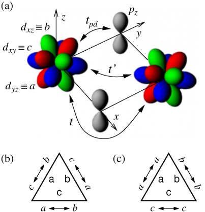
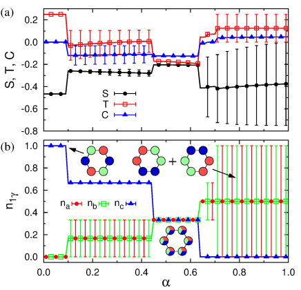
Fig. 13: Left — (a) Hopping processes between $t_{2g}$ orbitals along a bond parallel to the $c$ axis in NaTiO₂: (i) $t_{pd}$ between Ti($t_{2g}$) and O($2p_{z}$) orbitals — two $t_{pd}$ transitions define an effective hopping $t$, and (ii) direct $d-d$ hopping $t^{\prime}$. The $t_{2g}$ orbitals shown by different color are labeled as $a$, $b$, and $c$, see Eq. (2). The bottom part gives the hopping processes along $\gamma=a,b,c$ axes in the triangular lattice that contribute to Eq. (71): (b) superexchange and (c) direct exchange. Right — Ground state for a free hexagon as a function of $\alpha$ (71): (a) bond correlations — spin $S_{ij}$ Eq. (68) (circles), orbital $T_{ij}$ Eq. (69) (squares), and spin–orbital $C_{ij}$ Eq. (5.2) (triangles); (b) orbital electron densities $n_{1\gamma}$ at a representative site $i=1$ (left-most site): $n_{1a}$ (circles), $n_{1b}$ (squares), $n_{1c}$ (triangles). The insets indicate the orbital configurations favored by the superexchange ($\alpha=0$), by mixed $0.44<\alpha<0.63$, and by the direct exchange ($\alpha=1$). The vertical lines indicate an exact range due to the degeneracy. Images are reproduced from Ref. [40].

To explain the physical origin of the spin-orbital model for NaTiO₂ [39] we consider a representative bond along the $c$ axis shown in Fig. 13. For the realistic parameters of NaTiO₂ the $t_{2g}$ electrons are almost localized in $d^{1}$ configurations of Ti³⁺ ions, hence their interactions with neighboring sites can be described by the effective superexchange and kinetic exchange processes. Virtual charge excitations between the neighboring sites, $d_{i}^{1}d_{j}^{1}\rightleftharpoons d_{i}^{2}d_{j}^{0}$, generate magnetic interactions which arise from two different hopping processes for active $t_{2g}$ orbitals: ($i$) the effective hopping $t=t_{pd}^{2}/\Delta$ which occurs via oxygen $2p_{z}$ orbitals with the charge transfer excitation energy $\Delta$, in the present case along the 90^∘ bonds, and ($ii$) direct hopping $t^{\prime}$ which couples the $t_{2g}$ orbitals along the bond and give kinetic exchange interaction, as in the Hubbard model (1). Note that the latter processes couple orbitals with the same flavor, while the former ones couple different orbitals (for this geometry) so the occupied orbitals may be interchanged as a result of a virtual charge excitation — these processes are shown in Fig. 13.

The effective spin-orbital model considered here reads [39],

$${\cal H}=J\left\{(1-\alpha)\;{\cal H}_{s}+\sqrt{(1-\alpha)\alpha}\;{\cal H}_{m}+\alpha\;{\cal H}_{d}\right\}\,.$$ (71)

The parameter $\alpha$ in Eq. (71) is given by the hopping elements as follows,

$$\alpha=\frac{t^{\prime 2}}{t^{2}+t^{\prime 2}},$$ (72)

and interpolates between the superexchange ${\cal H}_{s}$ ($\alpha=0$) and kinetic exchange ${\cal H}_{d}$ ($\alpha=1$), while in between mixed exchange contributes as well; these terms are explained in Ref. [39]. This model is considered here in the absence of Hund’s exchange $\eta$ (26), i.e., at $\eta=0$. One finds that all the orbitals contribute equally in the entire range of $\alpha$, and each orbital state is occupied at two out of six sites in the entire regime of $\alpha$, see Fig. 13. The orbital state changes under increasing $\alpha$ and one finds four distinct regimes, with abrupt transitions between them. In the superexchange model ($\alpha=0$) there is precisely one orbital at each site which contributes, e.g. $n_{1c}=1$ as the $c$ orbital is active along both bonds. Having a frozen orbital configuration, the orbitals decouple from spins and the ground is disentangled, with $C_{ij}=0$, and one finds that the spin correlations $S_{ij}=-0.4671$, as for the AF Heisenberg ring of $L=6$ sites. Orbital fluctuations increase gradually with increasing $\alpha$ and this results in finite spin-orbital entanglement $C_{ij}\simeq-0.12$ for $0.10<\alpha<0.44$; simultaneously spin correlations weaken to $S_{ij}\simeq-0.27$.

In agreement with intuition, when $\alpha=0.5$ and all interorbital transitions shown in Fig. 13 have equal amplitude, there is large orbital mixing which is the most prominent feature in the intermediate regime of $0.44<\alpha<0.63$. Although spins are coupled by AF exchange, the orbitals fluctuate here strongly and reduce further spin correlations to $S_{ij}\simeq-0.21$. The orbital correlations are negative, $T_{ij}<0$, the spin-orbital entanglement is finite, $C_{ij}\simeq-0.13$, and the ground state is unique ($d=1$). Here all the orbitals contribute equally and $n_{1\gamma}=1/3$ which may be seen as a precursor of the spin-orbital liquid state which dominates the behavior of the triangular lattice. The regime of larger values of $\alpha>0.63$ is dominated by the kinetic exchange in Eq. (71), and the ground state is degenerate with $d=2$ [40], with strong scattering of possible electron densities $\{b_{i\gamma}\}$, see Fig. 13. Weak entanglement is found for $\alpha>0.63$, where $C_{ij}\simeq\neq 0$. Summarizing, except for the regimes of $\alpha<0.09$ and $\alpha>0.63$ the ground state of a single hexagon is strongly entangled, i.e., $C_{ij}<-0.10$, see Fig. 13.

5.3 Fractionalization of orbital excitations

As a rule, even when spin and orbital operators disentangle in the ground state, some of the excited states are characterized by spin-orbital entanglement. It is therefore even more subtle to separate spin-orbital degrees of freedom to introduce orbitons as independent orbital excitations, in analogy to the purely orbital model and the result presented in Fig. 3 [41]. This problem is not yet completely understood and we show here that in a 1D spin-orbital model the orbital excitation fractionalizes into freely propagating spinon and orbiton, in analogy to charge-spinon separation in the 1D $t$-$J$ model.

Fig. 14: Schematic representation of the orbital motion and the spin-orbital separation in a 1D spin-orbital model. The first hop of the excited state (a)$\to$(b) creates a spinon (wavy line) that moves via spin exchange $\propto J$. The next hop (b)$\to$(c) gives an orbiton freely propagating as a holon with an effective hopping $t\sim J/2$. Image is reproduced from Ref. [41].

While a hole doped to the FM chain propagates freely, it creates a spinon and a holon in an AF background described by the $t$-$J$ model. A similar situation occurs for an orbital excitation in AF/FO spin-orbital chain [41]. An orbital excitation may propagate through the system only after creating a spinon in the first step, see Figs. 14(a) and 14(b). The spinon itself moves via spin flips $\propto J>t$, faster than the orbiton, and the two excitations get well separated, see Fig. 14(c). The orbital-wave picture of Sec. 2, on the other hand, would require the orbital excitation to move without creating the spinon in the first step. Note that this would be only possible for imperfect Néel AF spin order. Thus one concludes that the symmetry between spin and orbital sector is broken also for this reason and orbitals are so strongly coupled to spin excitations in realistic spin-orbital models with AF/FO order that the mean field picture separating these two sectors of the Hilbert space breaks down.

6 $t$-$J$-like model for ferromagnetic manganites

Even more complex situations arise when charge degrees of freedom are added to spin-orbital models. The spectral properties of such models are beyond the scope of this discussion but we shall only point out that macroscopic doping changes radically spin-orbital superexchange by adding to it ferromagnetic exchange triggered by $e_{g}$ orbital liquid realized in hole doped manganites. As a result, the CMR effect is observed and the spin order changes to FM [3].

Similar to the spin case, the orbital Hubbard model Eq. (11) gives at large $\bar{U}\gg t$ the $e_{g}$ $t$-$J$ model [42], i.e., $e_{g}$ electrons may hop only in the restricted space without doubly occupied $e_{g}^{2}$ sites. The kinetic energy is gradually released with increasing doping $x$ in doped manganese oxides La${}_{1-x}A_{x}$MnO₃, with $A=$Sr,Ca,Pb, which is a driving mechanism for effective FM interaction generated by the kinetic energy $\propto{\tilde{H}}_{t}^{\uparrow}(e_{g})$ in the double exchange [3]. It competes with AF exchange which eventually becomes frustrated in FM metallic phase, arising typically at sufficient hole doping $x\simeq 0.17$. The evolution of magnetic order with increasing doping results from the above frustration: at low doping $x\sim 0.1$ AF spin order becomes stable and first changes to FM insulating phase, see Fig. 15(a). Only at larger doping $x$, an insulator-to-metal transition takes place which explains the CMR effect [3].

Fig. 15: Theoretical predictions for magnon spectra in the FM metallic phase in manganites: (a) spin-wave stiffness $D$ (solid line) as a function of hole doping $x$ given by double exchange (dashed) reduced by superexchange (SE) for: $A$-AF, FM insulating (FI), and FM metallic (FM) phases, and experimental points for La_1-xSr_xMnO₃ (diamonds) and La_0.7Pb_0.3MnO₃ (circle); empty circles for the hypothetical AO $|\pm\rangle$ state unstable against the $e_{g}$ orbital liquid; (b) magnon dispersion $\omega_{\vec{q}}$ obtained at $x=0.30$ (solid line) and the experimental points for La_0.7Pb_0.3MnO₃ [43] (circles and dashed line). Parameters: $U=5.9$, $J_{H}^{e}=0.7$, $t=0.41$, all in eV. Images are reproduced from Ref. [42].

In the FM metallic phase the magnon excitation energy is derived from manganite $t$-$J$ model and consists of two terms [42]: ($i$) superexchange being AF for the orbital liquid and ($ii$) FM double exchange $J_{\rm DE}$, proportional to the kinetic energy of $e_{g}$ electrons (6),

$$J_{\rm DE}=\frac{1}{2z{\cal S}^{2}}\,\left|\left\langle{\tilde{H}}_{t}^{\uparrow}(e_{g})\right\rangle\right|\,.$$ (73)

Here $z$ is the number of neighbors ($z=6$ for the cubic lattice), and $2{\cal S}=4-x$ is the average spin in a doped manganese oxide. The kinetic energy $\left|\left\langle{\tilde{H}}_{t}^{\uparrow}(e_{g})\right\rangle\right|$ measures directly the band narrowing due to the strong correlations in the $e_{g}$ orbital liquid. This explains why the spin-wave stiffness $D$ is: ($i$) reduced by the frustrating AF superexchange $J_{\rm SE}$ but ($ii$) increases proportionally to the hole doping $x$ in the FM metallic phase, see Fig. 15(a). As a result, the magnon dispersion in the FM metallic phase is given by,

$$\omega_{\vec{q}}=\left(J_{\rm DE}-J_{\rm SE}\right)z{\cal S}^{2}(1-\gamma_{\vec{q}}),$$ (74)

where $\gamma_{\vec{q}}=\frac{1}{z}\sum_{{\vec{\delta}}}e^{i{\vec{q}}\cdot{\vec{\delta}}}$, and ${\vec{\delta}}$ is a vector which connects the nearest neighbors.

An experimental proof that indeed the $e_{g}$ orbital liquid is responsible for isotropic spin excitations in the FM metallic phase of doped manganites we show the magnon spectrum observed in La_0.7Pb_0.3MnO₃, with rather large stiffness constant $D=7.25$ meV, see Fig. 15(b). Note that $D$ would be much smaller in the phase with AO order of $|\pm\rangle$ orbitals (28). Summarizing, the isotropy of the spin excitations in the simplest manganese oxides with FM metallic phase is naturally explained by the orbital liquid state of disordered $e_{g}$ orbitals.

7 Conclusions and outlook

Spin-orbital physics is a very challenging field in which only certain and mainly classical aspects have been understood so far. We have explained the simplest principles of spin-orbital models deciding about the physical properties of strongly correlated transition metal oxides with active orbital degrees of freedom. In the correlated insulators exchange interactions are usually frustrated and this frustration is released by certain type of spin-orbital order, with the complementarity of spin and orbital correlations at AF/FO or FM/AO bonds, as explained by the Goodenough-Kanamori rules [35].

One of the challenges is spin-orbital entanglement which becomes visible both in the ground and excited states. The coherent excitations such as magnons or orbitons are frequently not independent and also composite spin-orbital excitations are possible. Such excitations are not yet understood, except for some simplest cases as e.g. the 1D spin-orbital model with SU(4) symmetry where all these excitations are on equal footing and contribute to the entropy in the same way [44]. Such a perfect symmetry does not occur in nature however, and the orbital excitations are more complex due to finite Hund’s exchange interaction and, at least in some systems, orbital-lattice couplings. They may be a decisive factor explaining why spin-orbital liquids do not occur in certain models. For the same reason in the absence of geometrical frustration, the orbital liquid seems easier to obtain than the spin liquid.

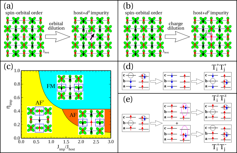
Fig. 16: Top — Doping by transition metal ions in an $ab$ plane with $C$-AF/$G$-AO order of $\{a,c\}$ orbitals found in $d^{4}$ Mott insulators (ruthenates) with: (a) orbital dilution by the $d^{3}$ impurity with $S=3/2$ spin, and (b) charge dilution by the $d^{2}$ impurity with $S=1$ spin. Host $S=1$ spins (red/black arrows) interact by $J_{\rm host}$ and doublons in $a$ ($c$) orbitals shown by green symbols. Here doping occurs at $a$ doublon site and spins are coupled by $J_{\rm imp}$ along hybrid (red) bonds. Bottom — (c) phase diagram for a single $d^{3}$ impurity replacing a doublon in $c$ orbital in the $C$-AF host [46], with changes in the orbital order indicated by dashed boxes (note $a\rightarrow b$ orbital flips); (d-e) orbital fluctuations promoted on $d^{2}$–$d^{4}$ hybrid bonds with (d) AF and (e) FM spin correlations. In the latter case (e) the doublons at two orbitals are coupled in excited states (doublon and hole in ovals), and one obtains orbital flips $\propto T_{i}^{-}T_{j}^{+}$ accompanied by Ising terms $\propto T_{i}^{z}T_{j}^{z}$, while double excitations $\propto T_{i}^{+}T_{j}^{+}$ occur on AF bonds (d) even in the absence of Hund’s exchange and are amplified by finite $\eta$. Image is reproduced from Ref. [47].

Doping of spin-orbital systems leads to very rich physics with phase transitions induced by moving charge carriers, as for instance in the well known example of the CMR manganites. Yet, the holes doped to the correlated insulators with spin-orbital order may be of quite different nature. Charge defects may prevent the holes from coherent propagation [45] and as a result the spin-orbital order will persist to rather high doping level.

Recently doping by transition metal ions with different valence was explored [46] — in such $t_{2g}$ systems local or global changes of spin-orbital order result from the complex interplay of spin-orbital degrees of freedom at orbital dilution, see Fig. 16(a). In general, the observed order in the doped system will then depend on the coupling between the ions with different valence compared with that within the host $J_{\rm imp}/J_{\rm host}$, and on Hund’s exchange at doped ions $\eta_{\rm imp}$. Not only a crossover between AF and FM spin correlations is expected with increasing $\eta_{\rm imp}$, but also the orbital state will change from inactive orbitals to orbital polarons on the hybrid bonds with increasing $J_{\rm imp}$, see Fig. 16(c). Quite a different case is given when double occupancies are replaced by empty orbitals in charge doping as shown in Fig. 16(b). Here orbital fluctuations are remarkably enhanced by the novel double excitation $\propto T_{i}^{+}T_{j}^{+}$ terms, see Figs. 16(d-e). On the one hand, large spin-orbital entanglement is expected in such cases when Hund’s exchange is weak, while on the other hand the superexchange will reduce to the orbital model in the FM regime. By mapping of this latter model to fermions one may expect interesting topological states in low dimension that are under investigation at present.

References

- [1] K.A. Chao, J. Spałek, and A.M. Oleś, J. Phys. C 10, L271 (1977)
- [2] M. Imada, A. Fujimori, and Y. Tokura, Rev. Mod. Phys. 70, 1039 (1998)
- [3] E. Dagotto, T. Hotta, and A. Moreo, Phys. Rep. 344, 1 (2001)
- [4] K.I. Kugel and D.I. Khomskii, Sov. Phys. Usp. 25, 231 (1982)
- [5] C. Slater and G.F. Koster, Phys. Rev. 94, 1498 (1954)
- [6] G. Khaliullin and S. Maekawa, Phys. Rev. Lett. 85, 3950 (2000)
- [7] Louis Felix Feiner and Andrzej M. Oleś, Phys. Rev. B 71, 144422 (2005)
- [8] A.M. Oleś, G. Khaliullin, P. Horsch, and L.F. Feiner, Phys. Rev. B 72, 214431 (2005)
- [9] J.S. Griffith, The Theory of Transition Metal Ions (Cambridge University Press, Cambridge, 1971)
- [10] Andrzej M. Oleś, Phys. Rev. B 28, 327 (1983)
- [11] J. van den Brink, P. Horsch, F. Mack, and A.M. Oleś, Phys. Rev. B 59, 6795 (1999)
- [12] A. van Rynbach, S. Todo, and S. Trebst, Phys. Rev. Lett. 105, 146402 (2010)
- [13] P. Czarnik, J. Dziarmaga, and A.M. Oleś, Phys. Rev. B 96, 014420 (2017)
- [14] Zohar Nussinov and Jeroen van den Brink, Rev. Mod. Phys. 87, 1 (2015)
- [15] L. Cincio, J. Dziarmaga, and A.M. Oleś, Phys. Rev. B 82, 104416 (2010)
- [16] Sandro Wenzel and Andreas M. Läuchli, Phys. Rev. Lett. 106, 197201 (2011)
- [17] P. Czarnik, J. Dziarmaga, and A.M. Oleś, Phys. Rev. B 93, 184410 (2016)
- [18] Giniyat Khaliullin, Prog. Theor. Phys. Suppl. 160, 155 (2005)
- [19] G. Khaliullin, P. Horsch, and A.M. Oleś, Phys. Rev. B 70, 195103 (2004)
- [20] L.F. Feiner, A.M. Oleś, and J. Zaanen, Phys. Rev. Lett. 78, 2799 (1997) J. Phys.: Condens. Matter 10, L555 (1998)
- [21] A.M. Oleś, L.F. Feiner, and J. Zaanen, Phys. Rev. B 61, 6257 (2000)
- [22] W. Brzezicki, J. Dziarmaga, and A.M. Oleś, Phys. Rev. Lett. 109, 237201 (2012)
- [23] Eva Pavarini, Erik Koch, and A.I. Lichtenstein, Phys. Rev. Lett. 101, 266405 (2008)
- [24] W. Brzezicki, J. Dziarmaga, and A.M. Oleś, Phys. Rev. B 87, 064407 (2013)
- [25] Louis Felix Feiner and Andrzej M. Oleś, Phys. Rev. B 59, 3295 (1999)
- [26] Eva Pavarini and Erik Koch, Phys. Rev. Lett. 104, 086402 (2010)
- [27] Mateusz Snamina and Andrzej M. Oleś, Phys. Rev. B 94, 214426 (2016)
- [28] N.N. Kovaleva, A.M. Oleś, A.M. Balbashov, A. Maljuk, D.N. Argyriou, G. Khaliullin, and B. Keimer, Phys. Rev. B 81, 235130 (2010)
- [29] S. Miyasaka, Y. Okimoto, and Y. Tokura, J. Phys. Soc. Jpn. 71, 2086 (2002)
- [30] Andrzej M. Oleś and Giniyat Khaliullin, Phys. Rev. B 84, 214414 (2011)
- [31] G. Khaliullin, P. Horsch, and A.M. Oleś, Phys. Rev. Lett. 86, 3879 (2001)
- [32] P. Horsch, A. M. Oleś, L. F. Feiner, and G. Khaliullin, Phys. Rev. Lett. 100, 167205 (2008)
- [33] S. Miyasaka, Y. Okimoto, M. Iwama, and Y. Tokura, Phys. Rev. B 68, 100406 (2003)
- [34] J. Fujioka, T. Yasue, S. Miyasaka, Y. Yamasaki, T. Arima, H. Sagayama, T. Inami, K. Ishii, and Y. Tokura, Phys. Rev. B 82, 144425 (2010)
- [35] J.B. Goodenough, Magnetism and the Chemical Bond (Interscience, New York, 1963)
- [36] K. Wohlfeld, M. Daghofer, and A.M. Oleś, Europhys. Lett. (EPL) 96, 27001 (2011)
- [37] Andrzej M. Oleś, J. Phys.: Condens. Matter 24, 313201 (2012)
- [38] Patrik Fazekas: Lecture Notes on Electron Correlation and Magnetism (World Scientific, Singapore, 1999)
- [39] Bruce Normand and Andrzej M. Oleś, Phys. Rev. B 78, 094427 (2008)
- [40] Jiří Chaloupka and Andrzej M. Oleś, Phys. Rev. B 83, 094406 (2011)
- [41] K. Wohlfeld, M. Daghofer, S. Nishimoto, G. Khaliullin, and J. van den Brink, Phys. Rev. Lett. 107, 147201 (2011)
- [42] Andrzej M. Oleś and Louis Felix Feiner, Phys. Rev. B 65, 052414 (2002)
- [43] J.A. Fernandez-Baca, P. Dai, H.Y. Hwang, C. Kloc, and S.-W. Cheong, Phys. Rev. Lett. 80, 4012 (1998)
- [44] B. Frischmuth, F. Mila, and M. Troyer, Phys. Rev. Lett. 82 835 (1999)
- [45] A. Avella, P. Horsch, and A.M. Oleś, Phys. Rev. Lett. 115, 206403 (2015)
- [46] W. Brzezicki, A.M. Oleś, and M. Cuoco, Phys. Rev. X 5, 011037 (2015)
- [47] W. Brzezicki, M. Cuoco, and A.M. Oleś, J. Supercond. Novel Magn. 30, 129 (2017)
Index
-
compass model §2
- generalized §2
- degenerate Hubbard model §1
- double exchange §6
- orbital Hubbard model §1
- orbital superexchange §2
- Goodenough-Kanamori rules §5.1
- Hund’s exchange §1
- Kugel-Khomskii model §3.2
- Mott insulator §1, §3.1
- on-site Coulomb interactions §1
- optical spectral weight §3.1, §3.3, §4.2
- quantum critical point Fig. 7, Fig. 8
- spin-orbital entanglement §5.2
- spin-orbital superexchange §3.1
- spinon-orbiton separation §5.3
- - model §1, §5.3, §6