X-ray Emission from SN 2012ca: A Type Ia-CSM Supernova Explosion in a Dense Surrounding Medium

Abstract

X-ray emission is one of the signposts of circumstellar interaction in supernovae (SNe), but until now, it has been observed only in core-collapse SNe. The level of thermal X-ray emission is a direct measure of the density of the circumstellar medium (CSM), and the absence of X-ray emission from Type Ia SNe has been interpreted as a sign of a very low density CSM. In this paper, we report late-time (500–800 days after discovery) X-ray detections of SN 2012ca in Chandra data. The presence of hydrogen in the initial spectrum led to a classification of Type Ia-CSM, ostensibly making it the first SN Ia detected with X-rays. Our analysis of the X-ray data favors an asymmetric medium, with a high-density component which supplies the X-ray emission. The data suggest a number density $>10^{8}$ cm^-3 in the higher-density medium, which is consistent with the large observed Balmer decrement if it arises from collisional excitation. This is high compared to most core-collapse SNe, but it may be consistent with densities suggested for some Type IIn or superluminous SNe. If SN 2012ca is a thermonuclear SN, the large CSM density could imply clumps in the wind, or a dense torus or disk, consistent with the single-degenerate channel. A remote possibility for a core-degenerate channel involves a white dwarf merging with the degenerate core of an asymptotic giant branch star shortly before the explosion, leading to a common envelope around the SN.

1 Introduction

Thermal X-ray emission is one of the clearest indications of circumstellar interaction in supernovae (SNe; Chevalier, 1982; Chevalier & Fransson, 1994). The intensity of the emission depends on the square of the density, and thus is a good estimator of the density of the ambient medium, as long as the emission is not absorbed by the medium. So far, over 60 SNe have been detected in X-rays (Dwarkadas & Gruszko, 2012; Dwarkadas, 2014). All of them are core-collapse SNe, where the circumstellar medium (CSM) is formed by mass loss from the progenitor star. Until now, no Type Ia SN has been detected in X-rays. Deep limits on the emission from SNe Ia in the radio (Chomiuk et al., 2016) and X-ray (Margutti et al., 2014) bands indicate a very low mass-loss rate ($\leq 10^{-9}$ M_⊙ yr^-1) for the stellar progenitor system, suggesting that SNe Ia are surrounded by a very low density CSM, if they even have one.

It is generally accepted that the progenitor of a SN Ia must be a white dwarf. In order to raise the mass of this white dwarf to nearly the Chandrasekhar limit to produce an explosion, it must have accreted mass transferred from a companion in a binary system. The nature of the companion is hotly debated (e.g., Ruiz-Lapuente, 2014), with evidence existing for both double-degenerate and single-degenerate systems (Maoz et al., 2014). In the former case, the companion is another white dwarf (Scalzo et al., 2010; Silverman et al., 2011; Nugent et al., 2011; Bloom et al., 2012; Brown et al., 2012), while in the latter case it is a main sequence or evolved star (Hamuy et al., 2003; Deng et al., 2004). It is likely that both channels are present.

Some SNe Ia exhibit narrow hydrogen lines superimposed on a SN Ia-like spectrum (Hamuy et al., 2003; Deng et al., 2004). The narrow line width suggests velocities much lower than that of the expanding shock wave, and are therefore presumed to arise in the surrounding medium. This indicates the presence of an ambient medium, perhaps arising from mass loss from the companion star. These SNe comprise the subclass of Type Ia-CSM. Silverman et al. (2013) composed a list of several common features of SNe Ia-CSM. The absolute magnitudes of SNe Ia-CSM are larger than those of normal SNe Ia. They even exceed those of most SNe IIn, whose spectra show relatively narrow lines (hence the “n” designation; see Filippenko (1997) for a review) on a broad base. The spectra of SNe Ia-CSM consist of a SN Ia spectrum diluted by relatively narrow hydrogen lines, a blue continuum created from many overlapping broad lines from iron-group elements, and strong H$\alpha$ emission with width $\sim 2000$ km s^-1. The H$\alpha$ profile varies for $\sim 100$ days post-explosion before steadily increasing. He I and H$\beta$ emission are observed, but are relatively weak. SNe Ia-CSM have larger Balmer decrements (the ratio of the intensity of the H$\alpha$ to H$\beta$ lines) than the typical value under interstellar conditions of $\sim 2.86$, most likely resulting from emission due to collisional excitation rather than recombination, suggesting high-density CSM shells that are collisionally excited when the faster-moving SN ejecta overtake them. SNe Ia-CSM have never been detected at radio wavelengths, and this work represents the first detection of a SN Ia-CSM in X-rays. The host galaxies of SNe Ia-CSM appear to be spiral galaxies having Milky-Way-like luminosities with solar metallicities, or irregular dwarf galaxies similar to the Magellenic Clouds with subsolar metallicities.

Since SNe Ia-CSM exhibit characteristic features of SNe Ia spectra with H lines that are the defining aspect of Type II SNe, there is still debate on their exact nature. Some suggest that they are odd core-collapse SNe masquerading as a SN Ia (Benetti et al., 2006). However, there are indications that some SNe Ia-CSM are likely thermonuclear explosions interacting with a CSM. PTF11kx is by most accounts a SN Ia produced from the single-degenerate channel (Dilday et al., 2012; Silverman et al., 2013). Observations of PTF11kx show the evolution of its spectrum to be similar to that of SN 1999aa, a SN Ia. It appears to have a multi-component CSM, with no signs of a CSM in the early-time observations. There exists faster-moving material closer to the SN, and shells of CSM (Dilday et al., 2012) expanding outward in radius from the SN. These features are interpreted by the authors as being consistent with recurrent nova eruptions, and thus suggest a thermonuclear explosion of a white dwarf through the single-degenerate channel.

SN 2012ca reignited the debate about whether all SNe Ia-CSM are thermonuclear explosions. While a thermonuclear progenitor is debated for SN 2012ca, its spectral classification is Type Ia with superimposed relatively narrow H lines. Inserra et al. (2014) argue that SN 2012ca is a core-collapse SN based on the identification of several intermediate-mass elements such as C, Mg, and O in its nebular spectrum. Furthermore, Inserra et al. (2016) point out that SN 2012ca is likely a core-collapse SN on the basis of energetics, suggesting that the conversion of kinetic energy into luminosity must be between 20% and 70%, an unusually large value. Fox et al. (2015) argue that the C, Mg, and O features seen by Inserra et al. (2014) are misidentified; instead, they suggest that those of Mg and O are actually iron lines, and that of C is the Ca II near-infrared (IR) triplet. Based on the lack of broad C, O, and Mg in the spectrum of SN 2012ca and the presence of broad iron lines, Fox et al. (2015) conclude that SN 2012ca is more consistent with a thermonuclear rather than a core-collapse explosion. They further point out that the high efficiency required for SN 2012ca is within the realm of possibility.

The goal of this paper is to further study the nature of SN 2012ca via its X-ray emission. Through the analysis of the X-ray data, we shed light on the density of the ambient medium and therefore the nature of the progenitor system. This paper is structured as follows. In §2, we summarize the X-ray data and analysis. In §3, we use the optical data to estimate the SN kinematics. In §4, we elaborate on the reduction and analysis of the spectra. An estimate of the density of the CSM, for both a homogeneous and a clumpy medium, is presented in §5. Finally, §6 summarizes our work and discusses the implications of the discovery.

2 Observations

SN 2012ca was discovered in the late-type spiral galaxy ESO 336-G009 on 2012 April 25.6 (Drescher et al., 2012). The NASA/IPAC Extragalactic Database (NED) gives the luminosity distance to the galaxy as 80.1 Mpc for a value of H${}_{0}=73$ km s^-1 Mpc^-1, $\Omega_{m}=0.27$, and $\Omega_{\Lambda}=0.73$. We observed SN 2012ca with the Chandra Advanced CCD Imaging Spectrometer (ACIS); see Table LABEL:table:12cadata for details. Two observations of 20 ks each were made about 6 months apart: ObsID 15632 (2013 September 17, hereafter epoch 1) and 15633 (2014 March 27, hereafter epoch 2). Using an explosion date of MJD $55998.2{\pm 20}$ (Inserra et al., 2016), these epochs occur 554 days and 745 days after the explosion, respectively. All epochs in this paper will be referenced from this explosion date, and all dates are listed in Universal Time (UT).

Table 1: Summary of X-ray data on SN 2012ca, listing the satellite and instrument which took the observation, the date, the age (days after explosion), the exposure time, the count rate, the column density, the derived temperature, and the unabsorbed flux, with 1$\sigma$ error bars where available.

Instrument	Obs Date	Days After	Exposure	Count Rate	$N_{\rm H}$	$kT$	0.5–7 keV
		Outburst	(ks)	($10^{-3}$	($10^{22}$	(keV)	Flux ($10^{-14}$
				counts s-1)	${\rm cm^{-2}}$)		erg s-1 cm-2)
Chandra ACIS	2013-09-17	554	20.0	1.4 $\pm 0.29$	6.0 $\pm 3.5$	$2.6\pm 1.8$	$7.6_{-5.1}^{+389}$
Chandra ACIS	2014-03-27	745	20.0	$0.29^{+0.26}_{-0.16}$	$5.2\pm 2.5$	$1.2\pm 0.5$	$3.7^{+104.0}_{-3.0}$

The data were analysed using Chandra Interactive Analysis of Observations (CIAO) version 4.7 and CalDB 4.8. The source and background regions were each taken to be $4^{\prime\prime}$ radius, which contains 90% of the Chandra point-spread function. Analysis and fitting were done using CIAO and Sherpa. Because the number of counts in each observation is low compared to the background, fitting methods involving minimizing the $\chi^{2}$ statistic are invalid. Instead, we used the “cstat” statistic, corresponding to the maximum likelihood function of the Poisson distribution, and fitted both the data and background together (Cash, 1979). While we used ungrouped spectra in our analysis, the grouped spectra for epochs 1 and 2 are shown in Figure 1.

We use the two optical spectra of SN 2012ca published by Fox et al. (2015) at 486 and 508 days after the explosion. The most recent spectra, on days 522.8, 548.9, 580.8, were obtained from WISeREP (Yaron & Gal-Yam, 2012) as part of the PESSTO SSDR2 (Smartt et al., 2015). We thank Dr. Cosimo Inserra for providing the rest of the optical spectra of SN 2012ca published by Inserra et al. (2014).

Figure 1: Left: X-ray spectrum at epoch 1. The data are grouped such that there are 4 counts per bin. Right: Spectrum for epoch 2, also grouped into 4 counts per bin. Although the grouped spectra are shown for clarity, ungrouped versions of these spectra were used in the analysis.

3 Supernova Kinematics

The velocity of the fast-moving gas is required for subsequent analysis. To determine this, we fit a cubic spline function to each H$\alpha$ profile in the optical spectra. This spectral fitting algorithm is similar to the one used by Silverman et al. (2012). We specifically recorded the velocity of the peak of the H$\alpha$ profile, as well as the blue-side width at zero intensity (BSWZI). All of the H$\alpha$ peaks have measured velocities consistent with 0 km s^-1 (in the rest frame of the host galaxy), and the velocity of the peak does not appear to evolve with time. As shown in Figure 2, the BSWZI is also measured to be approximately constant with time and has a value of $3200\pm 300$ km s^-1.

It is not clear if the BSWZI is representative of the shock velocity, since other factors could contribute to the broadening of the line. Electron scattering is one such factor, and has been shown to be relevant in SNe such as SN 2010jl (Fransson et al., 2014). However, it is unlikely that electron scattering could be important as late as 530 days, when the last optical spectra were obtained. The BSWZI also does not appear to change substantially in the first 500 days. Furthermore, the column density that we infer from the X-ray observations, although large, is still two orders of magnitude lower than that inferred for SN 2010jl (Fransson et al., 2014; Chandra et al., 2015), and would not lead to large electron scattering depths. Finally, electron scattering results in Lorentzian line shapes, whereas the line shapes here are better fitted by a Gaussian. Thus, we do not believe that electron scattering plays a large role. Other factors such as line blending or contamination from the reverse shock could be present. Therefore, although there is evidence of gas moving at velocities as high as 3200 km s^-1, we cannot easily assume that this represents the shock velocity.

The Gaussian shape of the lines indicates that there is material in the SN moving at all velocities from +3500 km s^-1 to $-3500$ km s^-1. We have also measured the full width at half-maximum intensity (FWHM) of the line from the two high-resolution spectra that we have, on days 436.2 and 458.1. The FWHM of the H$\alpha$ line is around 1300 km s^-1. The other spectra have low resolution, and measuring the FWHM is quite unreliable, even when corrected for instrument resolution. It is possible that the lower velocity is more indicative of the velocity of the bulk of the gas. We address this issue again in §5.

Figure 2: Blue-side width at zero intensity (BSWZI) of the H$\alpha$ line vs. time since explosion. The mean velocity indicated is $\sim 3200$ km s^-1.

4 Modeling the Spectrum

There are several indications of a high density in the surrounding medium: (1) the large Balmer decrement, which ranges from 3 to 20 for SN 2012ca, and can potentially be explained by collisional excitation rather than recombination, as for other Type Ia-CSM; (2) the slow velocity of the SN shock wave even at early times ($\la 3200$ km s^-1), compared to general SN Ia velocities in excess of $10^{4}$ km s^-1 (Wang et al., 2009); and (3) the high observed X-ray luminosity (see below) at a deduced redshift of $z=0.019$ (Inserra et al., 2014), generally seen in Type IIn SNe with high densities. In a high-density medium, thermal emission is expected to dominate. The low statistics make it difficult to robustly distinguish between nonthermal and thermal models, but the high density suggests that thermal models are a good starting point. We fit the X-ray spectrum with the “vmekal” model (Liedahl et al., 1995) using $z=0.019$, multiplied by the Tuebingen-Boulder model for X-ray absorption (Wilms et al., 2000). The background was fit with an 8-degree polynomial, and then the background plus data were simultaneously fit together, using the C-statistic to gauge the goodness of the fit.

Given the low statistics, it is difficult to accurately fit a model to the X-ray spectrum and extract relevant parameters, especially for the second epoch. Several models with different column densities and temperatures appear to provide a good fit. For example, we found two fits to epoch 2 which have reduced statistics of 0.5073 and 0.5071. The former has an $N_{\rm H}$ of $2.65\times 10^{22}$ cm^-2 and a $kT$ of 0.38 keV, while the latter has an $N_{\rm H}$ of $4.24\times 10^{22}$ cm^-2 and a $kT$ of 1.31 keV. To address this problem, we explore the likelihood parameter space with a modified Levenberg-Marquardt algorithm (Moré, 1979) to find many local minima which each provide a good fit to the data and are indisinguishable on statistical grounds. All such statistically indistinguishable local minima are shown in Figure 3, which was computed in the following manner. We first calculate the observed (absorbed) flux with 90% confidence error bars between 0.5 and 7 keV directly from the data using the CIAO srcflux command. At the first epoch the absorbed flux is $1.81^{0.9}_{-0.68}\times 10^{-14}$ erg cm^-2 s^-1, and at the second epoch the flux is $2.45^{+2.13}_{-1.35}\times 10^{-15}$ erg cm^-2 s^-1. We then attempted to fit the “vmekal” model to the X-ray spectrum 7000 different times. Each fit had different initial guesses for $N_{\rm H}$ and $kT$. The initial guesses for $N_{\rm H}$ ranged from $0.0882\times 10^{22}$ cm^-2 to $10\times 10^{22}$ cm^-2. The initial guesses for $kT$ ranged from 0.1 keV to 25 keV. We placed a lower bound on the column density ($N_{\rm H}$) of $0.0882\times 10^{22}$ cm^-2, which is the Galactic column density in the direction of SN 2012ca (Dickey & Lockman, 1990). We also placed a conservative upper bound on the temperature of 25 keV, slightly higher than the proton temperature for a shock velocity of $3500$ km s^-1.

For each fit, the model-dependent absorbed flux was computed using CIAO’s calc_energy_flux function. We rejected all fits for which the model-dependent absorbed flux was not within the 90% confidence interval of the model-independent flux. We then visually inspected the fits which passed this criteria to ensure that the model did not produce features which massively overestimated or underestimated the data in any energy range, and rejected all fits that gave a reduced test statistic exceeding 1. The final $N_{\rm H}$ and $kT$ values for acceptable fits are shown in Figure 3, which we treated as the parameter space of suitable values of $N_{\rm H}$ and $kT$.

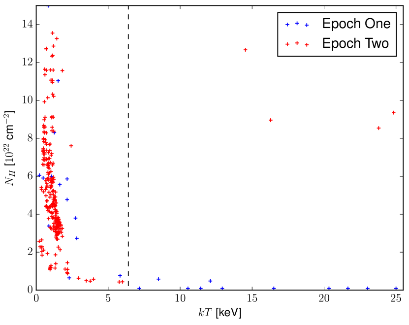
Figure 3: The red points (epoch 2) and blue points (epoch 1) represent acceptable X-ray spectral fit values for the column density ($N_{\rm H}$) and temperature ($kT$) for SN 2012ca, using the method outlined in the text. The points to the right of the dashed line are excluded from parameter estimation for reasons outlined in the text.

From Figure 3, fits to the X-ray spectrum for the second epoch cluster at low $kT$ and high $N_{\rm H}$. In contrast, the first epoch appears to have values that occupy two distinct regions: a region with low $N_{\rm H}$ and high $kT$, and a region with high $N_{\rm H}$ and low $kT$. This provides a clue to understanding the true best fits — since there is no obvious mechanism to add more material to the CSM as the SN evolves, we would expect the second epoch to have a lower value of $N_{\rm H}$ than the first, suggesting that the true $N_{\rm H}$ at the first epoch must be high, combined with a low $kT$.

Another clue to the correct fitting parameters is provided by the observed data. We can compute the electron number density $n_{e}$ directly from the X-ray luminosity $L=n_{e}^{2}\Lambda\,V$, given a cooling function $\Lambda$ and the volume of the emitting region $V$. Here we compute the minimum possible density and infer a constraint on $N_{\rm H}$. As a first guess, the minimum unabsorbed luminosity $L$ is calculated from the unabsorbed flux, which we determine from the observed count rate using the Galactic $N_{\rm H}$, the lowest possible value of $N_{\rm H}$. This is done with the Portable, Interactive Multi-Mission Simulator (PIMMS). Because unabsorbed flux and thus density decreases with temperature, a temperature of 12 keV is used as a conservative value to minimize the density calculation. The estimated unabsorbed fluxes are $2.0^{+1.0}_{-0.7}\times 10^{-14}$ erg cm^-2 s^-1 for epoch 1 and $2.6^{+2.3}_{-1.5}\times 10^{-15}$ erg cm^-2 s^-1 for epoch 2. This procedure gives luminosities of $1.48^{+0.74}_{-0.55}\times 10^{40}$ erg s^-1 for epoch 1, and $2.0^{+1.7}_{-1.1}\times 10^{39}$ erg s^-1 for epoch 2. Note that $\Lambda$ is an approximation of the cooling curve taken from Chevalier & Fransson (1994). The highest observed optical velocity is 3200 km s^-1, taken here to be the shock velocity, although it is possible that faster-moving material exists that is not observed at optical wavelengths because it has a lower emissivity, owing perhaps to a lower density. The radius is calculated assuming a shock velocity of $3200\pm 300$ km s^-1 and time since explosion. Since the inferred densities decrease with increasing shock velocity, by assuming the maximum observed gas velocity we minimize the inferred density. The shock is assumed to be strong and nonradiative to begin with because this is the simplest scenario, which can be tested and if necessary modified for consistency once we obtain a value for the density. We find that the minimum $n_{e}$ is $\sim 5.8^{+4.73}_{-1.8}\times 10^{6}$ cm^-3 at epoch 1, depending on the exact temperature, width of the shocked region, and shock velocity. The unshocked material has a density 4 times smaller for a strong shock. At epoch 2 the density of the shocked material is $\sim 1.4^{+1.44}_{-0.58}\times 10^{6}$ cm^-3. The cooling time for these densities and this temperature is much longer than the length of time between the explosion and observation, so our assumption of a nonradiative shock is self-consistent. This represents the absolute minimum luminosity and density. The density gives us an idea of what the minimum value of the column density should be, if integrated along the radius from the first observation to the second. Clearly, this indicates a very high column ${>5\times 10^{21}}$ cm^-2.

Because we do not have spectra before 50 days after the explosion, there is a possibility that the velocity of the shock was much higher than assumed for these first 50 days. In the worst case, the velocity is $10^{4}$ km s^-1, before sharply dropping to 3200 km s^-1. This would mean that the volume of material in the density calculation was underestimated, and thus our densities overestimated. In this worst-case scenario, our inferred shocked density for epoch 1 drops to $3.7^{+1.32}_{-1.05}\times 10^{6}$ cm^-3. For epoch 2, our inferred shocked density drops to $9.4^{+5.23}_{-3.92}\times 10^{5}$ cm^-3. The column density must still be $\ga 5\times 10^{21}$ cm^-2.

5 Calculating the Density of the CSM

5.1 Symmetric Medium

Keeping the above discussion in mind, we proceed to determine the actual fit parameters using Figure 3. We used a kernel density estimator with Gaussian kernels on the fits in Figure 3 to estimate the distributions for $N_{\rm H}$ and $kT$ for each epoch. We excluded all fits to epoch 1 in the high-$kT$ and low-$N_{\rm H}$ regime, those with $kT>6.4$ keV, because we have already determined that $N_{\rm H}>5\times 10^{21}$ cm^-2. We also excluded the fits to epoch 2 in the high-$kT$ and high-$N_{\rm H}$ region because $N_{\rm H}$ and $kT$ must be higher for epoch 1 than for epoch 2. To optimize the width of the Gaussian kernel, we performed the following procedure for a range of widths (Ivezić et al., 2014). First, we removed one point from the dataset. Next, we calculated the log of the likelihood of the density at the removed point. We repeated this step for each point. The sum of each log-likelihood divided by the number of fits was then used as a cost function. This cost function was minimized with respect to the width of the Gaussian kernel. We chose this cost function in order to minimize the estimator’s error between points, as the parameter space for epoch 1 is sparsely populated. For epoch 1, the width of the $kT$ kernel was 1.8 keV and the width of the $N_{\rm H}$ kernel was ${1.6}\times 10^{22}$ cm^-2. For epoch 2, the width of the $kT$ kernel was 0.15 keV and the width of the $N_{\rm H}$ kernel was ${0.15}\times 10^{22}$ cm^-2. From our distributions of temperature and column density, we calculated the expectation value and 68% confidence errors from the distribution. While the uncertainties may appear small, we emphasize that the full range of possible values is larger. A realistic value for epoch 1 is $kT=2.63_{-1.82}^{+1.80}$ keV and $N_{\rm H}=6.07_{-3.58}^{+3.46}\times 10^{22}$ cm^-2.

Taking the variation in all quantities into account, for epoch 1, this gives a flux of $7.57_{-5.11}^{+389}\times 10^{-14}$ erg cm^-2 s^-1, and thus a luminosity of $5.81_{-3.92}^{+298}\times 10^{40}$ erg s^-1. We assume, despite not knowing the true shock velocity, a strong nonradiative shock with velocity 3200 km s^-1. We use the same formula as in §4 to compute the number density of the unshocked region, which we find to be $3.46_{-1.44}^{+16.9}\times 10^{6}$ cm^-3 at epoch 1. The cooling time for this temperature and density is $\sim 1340$ days, greater than the length of time between the explosion and observation, so the assumption of a nonradiative shock is self-consistent.

At epoch 2, we have $kT=1.17_{-0.53}^{+0.37}$ keV and $N_{\rm H}=5.20_{-2.20}^{+2.48}\times 10^{22}$ cm^-2, which gives an unabsorbed flux of $3.68_{-3.05}^{+104.0}\times 10^{-14}$ erg cm^-2 s^-1. This results in a luminosity of $2.82^{+79.9}_{-2.34}\times 10^{40}$ erg s^-1 and an unshocked density of $1.22^{+5.03}_{-0.74}\times 10^{6}$ cm^-3. The cooling time for this temperature and density is $\sim 2340$ days, greater than the length of time between the explosion and observation, so the assumption of a nonradiative shock is self-consistent. Thus, realistically, the density of the surrounding medium is $\sim 4\times 10^{6}$ cm^-3 at epoch 1 and about a factor of 4 smaller at epoch 2.

Given an approximate mean molecular weight $\mu$ of 1, we can derive a mass density $\sim 5.8^{+28.3}_{-2.4}\times 10^{-18}$ g cm^-3 for epoch 1 and $\sim 2.0^{+8.5}_{-1.2}\times 10^{-18}$ g cm^-3 for epoch 2. Taking the value of $n_{e}$ at the radius at epoch 1 ($r_{1}$), and integrating $n_{e}$ along the line of sight from $r_{1}$ to the radius at epoch 2 ($r_{2}$), assuming a constant density profile, we find that $N_{\rm H}\approx 1.82\times 10^{22}$ cm^-2. If we assume that $n_{e}$ drops rapidly after $r_{1}$ to its value at $r_{2}$ and take the value of $n_{e}$ at $r_{2}$ as more representative, then we get a value of $N_{\rm H}$ lower by a factor of 3. In reality, it is probably somewhere between the two, or possibly greater due to material beyond $r_{2}$, and thus $>1\times 10^{22}$ cm^-2. If we assume the density at $r_{2}$ to be spread over the region all the way to at least $r_{2}$, there is $\sim 0.04$ M_⊙ of material around the SN between $r_{1}$ and $r_{2}$, a lower limit on the mass of the CSM. The density at $r_{1}$ increases this to 0.11 M_⊙. The actual value is again probably somewhere in between, suggesting that at least $\sim 0.1\pm 0.05$ M_⊙ of material is present around the SN.

In an ionised medium, the lower limit on $N_{\rm H}$ derived above may not be valid if some or all of the material is ionised. It is therefore worthwhile to check the ionisation state of the medium. Since there is no nearby photoionising source, it is the X-ray emission itself that tends to ionise the medium. We compute the ionisation parameter given by Kallman & McCray (1982), $\xi={L_{X}}/{n_{e}r^{2}}$. An ionisation parameter $\xi\ga 100$ indicates that elements such as C, N, and O are completely ionised, whereas ionisation of heavier elements such as S and Fe requires $\xi\ga 1000$ (Chevalier & Irwin, 2012). For epoch 1, $\xi=71.43_{-38.15}^{+703.83}$. For epoch 2, $\xi=54.72_{-34.78}^{+325.20}$. Our results show that the gas is far from being fully ionised and therefore this should not significantly affect the column density. Inferring the global ionisation state from $\xi$ may be more difficult. For a spherically symmetric medium and a steady-state wind (for example), $n_{e}\propto r^{-2}$, and $\xi$ is a constant that describes the global state of the medium. In the present scenario, we have no knowledge of the actual density variation with radius, and the geometry of the medium is likely not spherical as argued in the next section. In fact, using the densities inferred for the high-density component in the next section would reduce the ionisation parameter significantly, indicating an almost neutral medium, with the caveat that the covering fraction of the high-density component is unknown.

Since we are agnostic about the shock velocity for the first 50 days, we must assume it is $10^{4}$ km s^-1 during that time and calculate the density. In this worst-case scenario, our inferred density for epoch 1 drops to $2.16^{+10.12}_{-0.87}\times 10^{6}$ cm^-3. For epoch 2, our inferred density drops to $8.44^{+33.79}_{-5.05}\times 10^{5}$ cm^-3. The inferred minimum column density must still be $>1\times 10^{22}$ cm^-2.

5.2 Asymmetry in the Medium

The above calculations assume a spherically symmetric medium, which would be the simplest assumption. The calculations do, however, lead to a contradiction. The velocity indicated from the BSWZI, 3200 km s^-1, implies a post-shock proton temperature of 12–20 keV, depending on the mean molecular weight. The X-ray fits give an electron temperature on the order of 2 keV or less. However, the high densities implied by the above calculations would mean that Coulomb equilibration should be important. For number densities greater than $10^{6}$ cm^-3 and $T\approx 10^{7}$ K ($\sim 1$ keV), using Equation 3.6 of Fransson et al. (1996), the equilibration time is $<10$ days. The equilibration time for electrons and protons would be on the order of 2 days for epoch 1, so we would expect the electron and proton temperatures to be equilibrated.

One way to resolve this is to assume that the X-ray emission is not coming from the fastest-moving gas. This is not unreasonable, given that there is evidence in the Gaussian line profiles for gas moving at all velocities from $-3500$ km s^-1 to +3500 km s^-1. If most of the emission was coming from a thin shell of gas with a small velocity range, we would have seen more of a boxy line profile. This is best exemplified by the case of SN 1993J (Fransson et al., 2005), where the emission is inferred to arise from a thin shell having a small velocity range. Instead, we see profiles that can be fit with a Gaussian shape. Indeed, our high-resolution spectra suggest a FWHM of around 1300 km s^-1, indicating that there is sufficient material going at several hundred to a thousand km s^-1.

This indicates the possible existence of a two-phase medium. Part of the gas is traveling at speeds up to 3200 km s^-1, but is expanding into a lower-density medium. Given the temperatures from the X-ray fits, the X-ray emission arises from gas moving at velocities around $1157^{+346}_{-518}$ km s^-1 during the first observation and $773_{-219}^{+114}$ km s^-1 during the second observation. Thus, the X-ray emission must be arising within a medium where the shock velocity is lower than that of the forward shock, and therefore the density is correspondingly higher. In a single-degenerate scenario, the dense medium may be due to clumps in the surrounding environment, or a dense torus. A clumpy medium has been inferred for SN 2002ic from spectroscopic (Deng et al., 2004) and spectropolarimetric (Wang et al., 2004) observations. Most standard double-degenerate scenarios involving the merger of two white dwarfs would not produce a dense medium, but one special case proposed to explain H lines in SNe Ia via a double-degenerate scenario (Sparks & Stecher, 1974; Livio & Riess, 2003) results in a circumbinary cloud or common envelope around the SN. A surrounding disk is a possibility in both the single- and double-degenerate scenarios (Mochkovitch & Livio, 1990; Han & Podsiadlowski, 2006), although it is doubtful that the Mochkovitch & Livio (1990) model could explain the H lines. A circumstellar disk or torus is also an ingredient of binary evolution models of SNe Ia computed by Hachisu et al. (2008). If the clumps, torus, envelope, or disk are in pressure equilibrium with the surrounding material (which is not necessary in a transient situation), the velocity ratios of a factor of 3–4 would indicate that this medium was about 9–16 times denser than the interclump/interdisk medium.

The mass density of this high-density medium, $\rho_{\rm hd}$, can be estimated. A $\sim 1000$ km s^-1 shock moving into a medium of density $\sim 10^{7}$ cm^-3 would be radiative. Therefore, in this scenario we use the equation for a radiative shock to estimate the density, assuming that most of the emission from the radiative shock arises at X-ray energies:

$$L_{X}=0.5(\alpha\times 4\pi r^{2})\rho_{\rm hd}v_{\rm sh}^{3},$$ (1)

where we take $v_{sh}$ to be the velocity associated with the temperature given by the X-ray fits, and $\alpha\times 4\pi r^{2}$ is the area of the emitting region, taken as a fraction $\alpha\leq 1$ of the spherical emitting area $4\pi r^{2}$ . For epoch 1, $v_{\rm sh}=1157^{+346}_{-518}$ km s^-1, and for epoch 2, $v_{\rm sh}=773_{-219}^{+114}$ km s^-1. The radius, or the surface area, of the clumps/disk is not known. Given the X-ray temperatures we obtain, we set the radius assuming a constant velocity of $1157^{+346}_{-518}$ km s^-1 over 554 days. For the radius of the second observation, we assume the same constant velocity for the first 554 days and then a velocity of $773_{-219}^{+114}$ km s^-1 out to 745 days. We find $\rho_{\rm hd}=1.95^{+1977}_{-1.78}\times 10^{-16}{\alpha}^{-1}$ g cm^-3 and $\rho_{\rm hd}=3.10^{+562}_{-2.86}\times 10^{-16}{\alpha}^{-1}$ g cm^-3 for the first and second observations, respectively. These density values correspond to number densities of $1.16^{+1181}_{-1.06}\times 10^{8}{\alpha}^{-1}$ cm^-3 and $1.85^{+336}_{-1.70}\times 10^{8}{\alpha}^{-1}$ cm^-3 for the first and second observations, respectively. If the area is larger, the density will decrease correspondingly, and vice versa. The cooling time of both a 1157 km s^-1 shock and a 773 km s^-1 shock into a region with such a density is less than twenty days, so our assumption of a radiative shock is justified.

This model fits some aspects of the data better, and so may be preferable. While the lack of detailed information does not allow for accurate calculations, it is clear that the densities are possibly even higher than in the symmetrical case, as expected. However, they are consistent with densities suggested for other SNe Ia-CSM (Wang et al., 2004; Deng et al., 2004; Aldering et al., 2006). These high densities are also consistent with those required for collisional excitation to be responsible for the high Balmer decrement values (Drake & Ulrich, 1980), which require $n_{e}>10^{8}$ cm^-3.

6 Discussion and Conclusions

We describe here the X-ray emission from SN 2012ca, the first Type Ia-CSM SN to be detected in X-rays. Although the statistics preclude an accurate fit, there are several indicators that the SN is expanding in an extremely high density medium, with density exceeding $10^{6}$ cm^-3, and $>10^{8}$ cm^-3 in our preferred scenario. The high Balmer decrement seen in this SN, with values ranging from 3 to 20, has been interpreted in other SNe Ia-CSM as being most likely produced through excitation rather than recombination (Silverman et al., 2013), which requires a very high density medium, on the order of $n_{e}\approx 10^{8}$ cm^-3. The spectral fits to the X-ray data imply a large column density $>10^{22}$ cm^-2, consistent with a large CSM density. The relatively low shock velocity (3200 km s^-1 at early times) also suggests a density orders of magnitude higher than that of a normal SN Ia.

Although the data could be fit by a spherically symmetric medium, this does lead to a contradiction in that the electron and ion temperatures are quite different, whereas the low Coulomb equilibration time suggests that they should be similar. The difference between the post-shock proton temperature and the fitted electron temperatures could indicate that the X-ray emission does not arise from the fast-moving gas, but from slower-velocity gas expanding into a denser medium. The fact that the optical spectra indicate there is a large amount of gas moving at low velocities suggests that our low X-ray temperatures are correct. This dense medium could consist of high-density clumps, a dense torus, a dense equatorial disk, or a common envelope. The X-ray emission would arise from shocks, probably radiative, entering this dense medium. The existence of this dense medium renders most double-degenerate scenarios unviable, except perhaps for one which involves the degenerate core of an asymptotic giant branch (AGB) star that shed its H envelope in a merger with a companion white dwarf shortly before the explosion (Livio & Riess, 2003).

The BSWZI of the H$\alpha$ emission indicates that it arises from the main 3200 km s^-1 shock. This, however, presents a problem: it is unlikely that a nonradiative shock could give rise to such a level of Balmer emission. Using Chevalier & Raymond (1978), the ratio of H$\alpha$ power to shock power is of order 10^-6, which is much smaller than the observed H$\alpha$ luminosity (Fox et al., 2015). The emission is probably not due to a spherical shock— as noted earlier, this would result in a boxy line profile at the shock velocity that is not seen. A radiative shock could be inferred, but if we assume the X-ray luminosity to be the shock luminosity, the density inferred due to the high shock velocity (from Equation 1) is not enough to cool the shock in the required time. Thus, none of these solutions is particularly attractive, and there is an inherent lack of self-consistency in some of them. This suggests that the interaction is probably more complex than noted here, occurring presumably at different velocities and with variable-density ambient medium. We note that a similar problem also occurs in many SNe IIn.

Inserra et al. (2016) use the optical light curves to compute the mass of the CSM in SN 2012ca, finding 2.3–2.6 M_⊙. For the spherically symmetric case, our mass is only 0.1 M_⊙, much lower than their value. However, in the case of an asymmetric or clumpy medium, the densities of the high-density component are about two orders of magnitude greater. If this higher-density component has even a 10% filling factor, then we would expect a CSM mass in the asymmetric-medium model of $\sim 1$ M_⊙, which is more consistent with the value of Inserra et al. (2016). Thus, an additional factor in favor of the asymmetric-medium model is the higher CSM mass, which is more likely able to power the optical luminosity. The discrepancy in the computed masses is not significant, considering that Inserra et al. (2016) use an ejecta profile that is not appropriate for Type Ia SNe (Dwarkadas & Chevalier, 1998), and they do not make allowances for deviations from spherical symmetry and a clumpy medium. Their model also requires a kinetic energy input of 7–9 $\times 10^{51}$ erg, which is large even compared to that of other SNe Ia-CSM modelled by them.

While we are constrained by the available data, in §4 we computed the absolute minimum flux and thereby density, assuming merely the observed flux and the Galactic column density. We reiterate that these provide a minimum limit to the ambient number density of $>10^{6}$ cm^-3, and show clearly that it is still higher than is typical for most SNe after 1.5 yr, and in the range deduced for SNe Ia-CSM in general. In order for all the observations to be consistent thereafter, the final deduced density ranges seem quite appropriate.

The inferred densities from SN 2012ca are extremely high compared to those of other SNe Ia, which typically expand in much lower densities. However, they are consistent with those inferred for other members of the SN Ia-CSM subclass, with most showing indications of high-density surroundings (Silverman et al., 2013). Aldering et al. (2006) suggest that SN 2005gj, also identified as a SN Ia-CSM, had an ambient density $n_{e}>10^{8}$ cm^-3. Wang et al. (2004) suggest that SN 2002ic had a dense, clumpy, disk-like environment, with clumps of density $>10^{8}$ cm^-3 and sizes $5\times 10^{16}$ cm. This is quite similar to the picture envisioned here for SN 2012ca. Deng et al. (2004) also suggest a dense, clumpy, and aspherical circumstellar medium for SN 2002ic, with mass-loss rates as high as $10^{-2}$ v_w100 M_⊙ yr^-1, where v_w100 = v${}_{w}/100\;{\rm km\;s^{-1}}$, and v_w is the stellar wind velocity. The density is much higher than that around typical core-collapse SNe, and perhaps also the subclass of Type IIn SNe. Densities of up to $n_{e}\approx 10^{6}$ cm^-3 have been estimated for the Type IIn SN 2006jd (Chandra et al., 2012), and between $3\times 10^{6}$ and $10^{8}$ cm^-3 for SN 2010jl (Fransson et al., 2014). High mass-loss rates have been found for SN 2005kd (Dwarkadas et al., 2016) and SN 2005ip (Katsuda et al., 2014). A clumpy medium has been suggested for Type IIn SNe such as SN 1988Z, SN 1978K, and SN 1986J (Chugai, 1993; Chugai & Danziger, 1994; Chugai et al., 1995), and a dense torus for SNe 2005kd, 2006jd, and 2010jl (Katsuda et al., 2016). SNe IIn in general have high X-ray luminosities (Figure 4; Dwarkadas & Gruszko, 2012; Dwarkadas, 2014; Chandra et al., 2015; Dwarkadas et al., 2016), which if due to thermal emission suggest high densities. Note that the luminosity predicted for SN 2012ca, of order $10^{40}$ erg s^-1, places it squarely within the range of the X-ray luminosities of SNe IIn (Figure 4; Dwarkadas & Gruszko, 2012; Dwarkadas et al., 2016). Despite these similarities, the temperature of SN 2012ca is significantly lower than that of most SNe IIn at a similar epoch. It typically takes SNe IIn a few thousand days to reach such low temperatures. The high CSM density around SN 2012ca may allow it to cool more quickly, explaining this discrepancy. Thus, while the spectra suggest a Type Ia SN, the X-ray luminosity, high density, and circumstellar interaction are typical of a core-collapse Type IIn SNe, suggesting a CSM similar to that seen in SNe IIn.

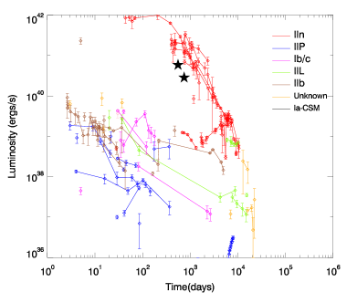
Figure 4: The X-ray light curves of most X-ray SNe, grouped by type. Adapted from Dwarkadas (2014), with SN 2012ca and some other data points added. The stars represent the nominal X-ray luminosities at the two epochs for SN 2012ca. Note that these place it in the middle of the range for SNe IIn.

While SN 2012ca is the first Type Ia-CSM SN to be detected in X-rays, others have been examined unsuccessfully for signs of X-ray emission. Hughes et al. (2007) took deep X-ray observations of SN 2002ic and SN 2005gj and placed upper limits on their X-ray flux. The limits on SN 2005gj are more stringent. The redshift 0.019 of SN 2012ca places it much closer than SN 2002ic ($z=0.0667$) and SN 2005gj ($z=0.062$). If SN 2012ca had occurred at the redshift of SN 2002ic, it would not have been detected. If it had occurred at the redshift of SN 2005gj, it may have been detected if it was cooler than 10 keV and the absorption of X-ray flux by the CSM was not significant. However, given the density estimate by Aldering et al. (2006), absorption in SN 2005gj could be higher than in SN 2012ca, making it undetectable. Furthermore, these SNe were observed at earlier epochs than SN 2012ca: SN 2002ic was observed 275 days after the explosion, while SN 2005gj was observed merely 81 days after the explosion. The column densities would have been much larger for similar external densities, thus contributing to making them undetectable.

It is not clear how the surrounding medium is produced, and furthermore what its density profile looks like. White dwarfs are not expected to experience any mass loss or have a high-density medium surrounding them. However, there are several scenarios for single-degenerate progenitors which produce an asymmetric dense medium via the companion. Single-degenerate scenarios could produce a clumpy medium, a dense torus, or a dense disk. Double-degenerate scenarios would not generally be expected to produce a H-rich dense medium, although one model does predict a H-rich circumbinary cloud or common envelope.

If the density profile is due to a stellar wind with constant mass-loss parameters $\rho_{\rm CSM}={\dot{M}}/{4\pi r^{2}v_{w}}$, where $\dot{M}$ is the mass-loss rate and $v_{w}$ the wind velocity, then for epoch 1, $\dot{M}/v_{w}$ must be larger than $2.7\times 10^{-4}$ v_w10 M_⊙ yr^-1 in the spherically symmetric case, and two orders of magnitude larger in the two-component medium case (although asphericity may increase it further). Despite being extremely high, this mass-loss rate is consistent with those derived from light-curve modelling of SNe 2002ic and 1997cy (Chugai & Yungelson, 2004), as well as that derived from spectral modelling of SN 2002ic (Kotak et al., 2004). This lower limit is orders of magnitude larger than upper limits derived from deep X-ray observations of nearby SNe Ia. Margutti et al. (2012) place an upper limit on $\dot{M}/v_{w}$ for the nearby Type Ia SN 2011fe of $2\times 10^{-10}$ v_w10 M_⊙ yr^-1, while Margutti et al. (2014) posit an upper limit on SN 2014J of $2.5\times 10^{-10}$ v_w10 M_⊙ yr^-1. Of course, the constant velocity over at least 500 days suggests that if there is a wind medium, its density is not decreasing as steeply as $r^{-2}$ but more gently (Dwarkadas & Gruszko, 2012).

This mass-loss rate may only be satisfied by the higher end of red supergiant stars (Mauron & Josselin, 2011) and by yellow hypergiant stars. If the surrounding velocity is higher, say 100-1000 km s^-1, then the mass-loss rate increases accordingly. This would then require a luminous blue variable (LBV) undergoing eruptive mass loss (Smith, 2014). Other SN progenitors such as Wolf-Rayet (W-R) stars have winds of $\sim 2000$ km s^-1, and would therefore require a mass-loss rate 100 times higher than that postulated above, which is orders of magnitude higher than those actually measured for W-R stars (Moffat, 2015). In addition, the presence of an H-rich medium immediately around the star effectively rules out W-R stars.

It must be pointed out here that having a high-mass secondary likely seems implausible around a white dwarf, given that one would have expected the higher-mass companion to have evolved faster and therefore be long gone before the white dwarf made an appearance. The only lower-mass ($<8$ M_⊙) progenitor that may be able to satisfy the high mass-loss rates for at least a short period would be an asymptotic giant branch star.

The ambient medium may not result from a freely expanding wind at all, but could be the result of a swept-up medium due to interacting winds (Dwarkadas, 2011), as suggested for SN 1996cr (Dwarkadas et al., 2010). In this case, the two winds do not need to have very high mass-loss rates, as long as there is sufficient mass for the later wind to sweep up. However, this would mean a low density very near the star, yet the low velocity shortly after explosion seems to argue against this.

An ambient medium owing to recurrent nova eruptions was suggested by Dilday et al. (2012) for PTF11kx. In that case, the presence of multiple components, with fast-moving material inside denser and slower-moving shells, could be explained by the SN shock interacting with shells of material resulting from episodic nova eruptions. It is not clear if such a model could apply here, since the SN shock maintains a low velocity that does not vary much over the first 550 days (see Figure 1).

Kepler’s SN remnant is a possible Galactic example of a SN Ia that requires dense mass loss. However, the CSM of Kepler’s SN remnant is much farther out than that of SN 2012ca (Reynolds et al., 2007; Katsuda et al., 2015). Katsuda et al. (2015) argue that Kepler’s SN was a highly overluminous SN Ia, and that the CSM consists of tenuous gas with dense knots, similar to the model outlined herein. Their analysis suggests that the knots were parsecs away from the progenitor, and the medium shows evidence of CNO processing — so, although both require a SN Ia progenitor and dense surrounding medium, the two events are not directly comparable. They infer a high mass-loss rate of $10^{-5}$ yr^-1, which is considerably larger than the upper limits quoted above, although lower than that inferred for SN 2012ca, especially in the asymmetric-medium scenario. Their models require a progenitor with a high mass-loss rate and no surviving companion; a recurrent-nova scenario is not favored for Kepler’s SN. The core-degenerate scenario laid out by Livio & Riess (2003) and elaborated further by Tsebrenko & Soker (2013) could be the origin of Kepler’s SN remnant. The supersoft channel investigated by Han & Podsiadlowski (2006) also remains a possibility.

Finally, as noted earlier, it is possible that this SN, and others like it, are not part of the class of SNe Ia at all. They most closely resemble SNe IIn, which presumably have more than one progenitor, all of the core-collapse variety. That, however, then leads to the question of why spectra of SNe Ia-CSM resemble those of the SN Ia class the most, and how the explosion of a massive star could give rise to SN Ia-like spectral features.

Notwithstanding its origin, the high density surrounding SN 2012ca is indisputable. The SN is fading in X-rays, and unlikely to be detectable any more by current instruments. However, it makes a clear case for other SNe Ia-CSM to be observed in X-rays, and presumably at radio wavelengths as well, opening up a new window to understanding this class of intriguing objects and unraveling the mystery of their progenitors. Continued long-term observations would also be useful to show if SNe of this class eventually evolve into remnants resembling that of Kepler’s SN.

References

- Aldering et al. (2006) Aldering G., Antilogus P., Bailey S., Baltay C., Bauer A., Blanc N., Bongard S., Copin Y., Gangler E., Gilles S., Kessler R., Kocevski D., Lee B. C., Loken S. e. a., 2006, ApJ, 650, 510
- Benetti et al. (2006) Benetti S., Cappellaro E., Turatto M., Taubenberger S., Harutyunyan A., Valenti S., 2006, ApJL, 653, L129
- Bloom et al. (2012) Bloom J. S., Kasen D., Shen K. J., Nugent P. E., Butler N. R., Graham M. L., Howell D. A., Kolb U., Holmes S., Haswell C. A., Burwitz V., Rodriguez J., Sullivan M., 2012, ApJL, 744, L17
- Brown et al. (2012) Brown P. J., Dawson K. S., de Pasquale M., Gronwall C., Holland S., Immler S., Kuin P., Mazzali P., Milne P., Oates S., Siegel M., 2012, ApJ, 753, 22
- Cash (1979) Cash W., 1979, ApJ, 228, 939
- Chandra et al. (2012) Chandra P., Chevalier R. A., Chugai N., Fransson C., Irwin C. M., Soderberg A. M., Chakraborti S., Immler S., 2012, ApJ, 755, 110
- Chandra et al. (2015) Chandra P., Chevalier R. A., Chugai N., Fransson C., Soderberg A. M., 2015, ApJ, 810, 32
- Chevalier (1982) Chevalier R. A., 1982, ApJ, 259, 302
- Chevalier & Fransson (1994) Chevalier R. A., Fransson C., 1994, ApJ, 420, 268
- Chevalier & Irwin (2012) Chevalier R. A., Irwin C. M., 2012, ApJL, 747, L17
- Chevalier & Raymond (1978) Chevalier R. A., Raymond J. C., 1978, ApJL, 225, L27
- Chomiuk et al. (2016) Chomiuk L., Soderberg A. M., Chevalier R. A., Bruzewski S., Foley R. J., Parrent J., Strader J., Badenes C., Fransson C., Kamble A., Margutti R., Rupen M. P., Simon J. D., 2016, ApJ, 821, 119
- Chugai (1993) Chugai N. N., 1993, ApJL, 414, L101
- Chugai & Danziger (1994) Chugai N. N., Danziger I. J., 1994, MNRAS, 268, 173
- Chugai et al. (1995) Chugai N. N., Danziger I. J., della Valle M., 1995, MNRAS, 276, 530
- Chugai & Yungelson (2004) Chugai N. N., Yungelson L. R., 2004, Astronomy Letters, 30, 65
- Deng et al. (2004) Deng J., Kawabata K. S., Ohyama Y., Nomoto K., Mazzali P. A., Wang L., Jeffery D. J., Iye M., Tomita H., Yoshii Y., 2004, ApJL, 605, L37
- Dickey & Lockman (1990) Dickey J. M., Lockman F. J., 1990, ARAA, 28, 215
- Dilday et al. (2012) Dilday B., Howell D. A., Cenko S. B., Silverman J. M., Nugent P. E., Sullivan M., Ben-Ami S., Bildsten L., Bolte M., Endl M., Filippenko A. V., Gnat O., Horesh A., Hsiao E. e. a., 2012, Science, 337, 942
- Drake & Ulrich (1980) Drake S. A., Ulrich R. K., 1980, ApJS, 42, 351
- Drescher et al. (2012) Drescher C., Parker S., Brimacombe J., 2012, Central Bureau Electronic Telegrams, 3101, 1
- Dwarkadas (2011) Dwarkadas V. V., 2011, MNRAS, 412, 1639
- Dwarkadas (2014) Dwarkadas V. V., 2014, MNRAS, 440, 1917
- Dwarkadas & Chevalier (1998) Dwarkadas V. V., Chevalier R. A., 1998, ApJ, 497, 807
- Dwarkadas et al. (2010) Dwarkadas V. V., Dewey D., Bauer F., 2010, MNRAS, 407, 812
- Dwarkadas & Gruszko (2012) Dwarkadas V. V., Gruszko J., 2012, MNRAS, 419, 1515
- Dwarkadas et al. (2016) Dwarkadas V. V., Romero-Cañizales C., Reddy R., Bauer F. E., 2016, MNRAS, 462, 1101
- Filippenko (1997) Filippenko A. V., 1997, ARAA, 35, 309
- Fox et al. (2015) Fox O. D., Silverman J. M., Filippenko A. V., Mauerhan J., Becker J., Borish H. J., Cenko S. B., Clubb K. I., Graham M. e. a., 2015, MNRAS, 447, 772
- Fransson et al. (2005) Fransson C., Challis P. M., Chevalier R. A., Filippenko A. V., Kirshner R. P., Kozma C., Leonard D. C., Matheson T., Baron E., Garnavich P., Jha S., Leibundgut B., Lundqvist P., Pun C. S. J., Wang L., Wheeler J. C., 2005, ApJ, 622, 991
- Fransson et al. (2014) Fransson C., Ergon M., Challis P. J., Chevalier R. A., France K., Kirshner R. P., Marion G. H., Milisavljevic D., Smith N., Bufano F., 2014, ApJ, 797, 118
- Fransson et al. (1996) Fransson C., Lundqvist P., Chevalier R. A., 1996, ApJ, 461, 993
- Hachisu et al. (2008) Hachisu I., Kato M., Nomoto K., 2008, ApJ, 679, 1390
- Hamuy et al. (2003) Hamuy M., Phillips M. M., Suntzeff N. B., Maza J., González L. E., Roth M., Krisciunas K., Morrell N., Green E. M., Persson S. E., McCarthy P. J., 2003, Nature, 424, 651
- Han & Podsiadlowski (2006) Han Z., Podsiadlowski P., 2006, MNRAS, 368, 1095
- Hughes et al. (2007) Hughes J. P., Chugai N., Chevalier R., Lundqvist P., Schlegel E., 2007, ApJ, 670, 1260
- Inserra et al. (2016) Inserra C., Fraser M., Smartt S. J., Benetti S., Chen T.-W., Childress M., Gal-Yam A., Howell D. A., Kangas T., Pignata G., Polshaw J., Sullivan M., Smith K. W., Valenti S., Young D. R., Parker S., Seccull T., McCrum M., 2016, MNRAS, 459, 2721
- Inserra et al. (2014) Inserra C., Smartt S. J., Scalzo R., Fraser M., Pastorello A., Childress M., Pignata G., Jerkstrand A., Kotak R., Benetti S. e. a., 2014, MNRAS, 437, L51
- Ivezić et al. (2014) Ivezić Ž., Connelly A. J., VanderPlas J. T., Gray A., 2014, Statistics, Data Mining, and Machine Learning in Astronomy
- Kallman & McCray (1982) Kallman T. R., McCray R., 1982, ApJS, 50, 263
- Katsuda et al. (2016) Katsuda S., Maeda K., Bamba A., Terada Y., Fukazawa Y., Kawabata K., Ohno M., Sugawara Y., Tsuboi Y., Immler S., 2016, ApJ, 832, 194
- Katsuda et al. (2014) Katsuda S., Maeda K., Nozawa T., Pooley D., Immler S., 2014, ApJ, 780, 184
- Katsuda et al. (2015) Katsuda S., Mori K., Maeda K., Tanaka M., Koyama K., Tsunemi H., Nakajima H., Maeda Y., Ozaki M., Petre R., 2015, ApJ, 808, 49
- Kotak et al. (2004) Kotak R., Meikle W. P. S., Adamson A., Leggett S. K., 2004, MNRAS, 354, L13
- Liedahl et al. (1995) Liedahl D. A., Osterheld A. L., Goldstein W. H., 1995, ApJL, 438, L115
- Livio & Riess (2003) Livio M., Riess A. G., 2003, ApJL, 594, L93
- Maoz et al. (2014) Maoz D., Mannucci F., Nelemans G., 2014, ARAA, 52, 107
- Margutti et al. (2014) Margutti R., Parrent J., Kamble A., Soderberg A. M., Foley R. J., Milisavljevic D., Drout M. R., Kirshner R., 2014, ApJ, 790, 52
- Mauron & Josselin (2011) Mauron N., Josselin E., 2011, AA, 526, A156
- Mochkovitch & Livio (1990) Mochkovitch R., Livio M., 1990, AA, 236, 378
- Moffat (2015) Moffat A. F. J., 2015, in Hamann W.-R., Sander A., Todt H., eds, Wolf-Rayet Stars: Proceedings of an International Workshop held in Potsdam, Germany, 1-5 June 2015. Edited by Wolf-Rainer Hamann, Andreas Sander, Helge Todt. Universitätsverlag Potsdam, 2015., p.13-18 General overview of Wolf-Rayet stars. pp 13–18
- Moré (1979) Moré J. J., 1979, Lecture Notes in Mathematics 630: Numerical Analysis, pp 105–116
- Nugent et al. (2011) Nugent P. E., Sullivan M., Cenko S. B., Thomas R. C., Kasen D., Howell D. A., Bersier D., Bloom J. S., Kulkarni S. R., Kandrashoff M. T., Filippenko A. V., Silverman J. M., Marcy G. W. e. a., 2011, Nature, 480, 344
- Reynolds et al. (2007) Reynolds S. P., Borkowski K. J., Hwang U., Hughes J. P., Badenes C., Laming J. M., Blondin J. M., 2007, ApJL, 668, L135
- Ruiz-Lapuente (2014) Ruiz-Lapuente P., 2014, New Atronomy Reviews, 62, 15
- Scalzo et al. (2010) Scalzo R. A., Aldering G., Antilogus P., Aragon C., Bailey S., Baltay C., Bongard S., Buton C., Childress M., Chotard N., Copin Y., Fakhouri H. K., Gal-Yam A., Gangler E. e. a., 2010, ApJ, 713, 1073
- Silverman et al. (2011) Silverman J. M., Ganeshalingam M., Li W., Filippenko A. V., Miller A. A., Poznanski D., 2011, MNRAS, 410, 585
- Silverman et al. (2012) Silverman J. M., Kong J. J., Filippenko A. V., 2012, MNRAS, 425, 1819
- Silverman et al. (2013) Silverman J. M., Nugent P. E., Gal-Yam A., Sullivan M., Howell D. A., Filippenko A. V., Arcavi I., Ben-Ami S., Bloom J. S., Cenko S. B., Cao Y., Chornock R. e. a., 2013, ApJS, 207, 3
- Silverman et al. (2013) Silverman J. M., Nugent P. E., Gal-Yam A., Sullivan M., Howell D. A., Filippenko A. V., Pan Y.-C., Cenko S. B., Hook I. M., 2013, ApJ, 772, 125
- Smartt et al. (2015) Smartt S. J., Valenti S., Fraser M., Inserra C., Young D. R., Sullivan M., Pastorello A., Benetti S., Gal-Yam A., Knapic C., Molinaro M., Smareglia R., Smith K. W. e. a., 2015, AA, 579, A40
- Smith (2014) Smith N., 2014, ARAA, 52, 487
- Sparks & Stecher (1974) Sparks W. M., Stecher T. P., 1974, ApJ, 188, 149
- Tsebrenko & Soker (2013) Tsebrenko D., Soker N., 2013, MNRAS, 435, 320
- Wang et al. (2004) Wang L., Baade D., Höflich P., Wheeler J. C., Kawabata K., Nomoto K., 2004, ApJL, 604, L53
- Wang et al. (2009) Wang X., Filippenko A. V., Ganeshalingam M., Li W., Silverman J. M., Wang L., Chornock R., Foley R. J., Gates E. L., Macomber B., Serduke F. J. D., Steele T. N., Wong D. S., 2009, ApJL, 699, L139
- Wilms et al. (2000) Wilms J., Allen A., McCray R., 2000, ApJ, 542, 914
- Yaron & Gal-Yam (2012) Yaron O., Gal-Yam A., 2012, PASP, 124, 668