The distribution of shortest path lengths in a class of node duplication network models

Abstract

We present analytical results for the distribution of shortest path lengths (DSPL) in a network growth model which evolves by node duplication (ND). The model captures essential properties of the structure and growth dynamics of social networks, acquaintance networks and scientific citation networks, where duplication mechanisms play a major role. Starting from an initial seed network, at each time step a random node, referred to as a mother node, is selected for duplication. Its daughter node is added to the network, forming a link to the mother node, and with probability $p$ to each one of its neighbors. The degree distribution of the resulting network turns out to follow a power-law distribution, thus the ND network is a scale-free network. To calculate the DSPL we derive a master equation for the time evolution of the probability $P_{t}(L=\ell)$, $\ell=1,2,\dots$, where $L$ is the distance between a pair of nodes and $t$ is the time. Finding an exact analytical solution of the master equation, we obtain a closed form expression for $P_{t}(L=\ell)$. The mean distance, $\langle L\rangle_{t}$, and the diameter, $\Delta_{t}$, are found to scale like $\ln t$, namely the ND network is a small world network. The variance of the DSPL is also found to scale like $\ln t$. Interestingly, the mean distance and the diameter exhibit properties of a small world network, rather than the ultrasmall world network behavior observed in other scale-free networks, in which $\langle L\rangle_{t}\sim\ln\ln t$.

I Introduction

The increasing interest in the field of complex networks in recent years is motivated by the realization that a large variety of systems and processes in physics, chemistry, biology, engineering, and society can be usefully described by network models Albert2002 ; Caldarelli2007 ; Havlin2010 ; Newman2010 ; Estrada2011b ; Barrat2012 . These models consist of nodes and edges, where the nodes represent physical objects, while the edges represent the interactions between them. It was found that networks appearing in different contexts often share various structural properties. For example, they exhibit repeating network motifs such as the feed-forward loop (FFL) and the auto-regulator Milo2002 ; Alon2006 . The structure of these motifs and their abundance provide useful information on the growth mechanism of the network and often has functional importance. At the global scale, many of these networks are scale-free, which means that they exhibit power-law degree distributions of the form $P(K=k)\sim k^{-\gamma}$ Barabasi1999 ; Jeong2000 ; Krapivsky2000 ; Krapivsky2001 ; Vazquez2003 . The most highly connected nodes, called hubs, play a dominant role in dynamical processes on these networks. A central feature of random networks is the small-world property, namely the fact that the mean distance and the diameter scale like $\ln N$, where $N$ is the network size Milgram1967 ; Watts1998 ; Chung2002 ; Chung2003 . Moreover, it was shown that scale-free networks are generically ultrasmall, namely their mean distance and diameter scale like $\ln\ln N$ Cohen2003 .

While pairs of adjacent nodes exhibit direct interactions, the interactions between most pairs of nodes are indirect, and are mediated by intermediate nodes and edges. Pairs of nodes may be connected by many different paths. The shortest among these paths are of particular importance because they are likely to provide the fastest and strongest interactions. Therefore, it is of much interest to study the distribution of shortest path lengths (DSPL) between pairs of nodes in different types of networks. Such distributions, which are also referred to as distance distributions, are expected to depend on the network structure and size. They are of great importance for the temporal evolution of dynamical processes Barrat2012 such as signal propagation in genetic regulatory networks Giot2003 ; Maayan2005 , navigation Dijkstra1959 ; Delling2009 and epidemic spreading Satorras2015 . Central measures of the DSPL such as the mean distance and extremal measures such as the diameter were studied Bollobas2001 ; Durrett2007 ; Watts1998 ; Fronczak2004 ; Newman2001b . However, apart from a few studies Newman2001 ; Dorogotsev2003 ; Blondel2007 ; Hofstad2007 ; Esker2008 ; Shao2008 ; Shao2009 , the DSPL has not attracted nearly as much attention as the degree distribution. Recently, an analytical approach was developed for calculating the DSPL Katzav2015 in the Erdős-Rényi (ER) network Erdos1959 , which is the simplest mathematical model of a random network. More general formulations were later developed Nitzan2016 ; Melnik2016 , for the broader class of configuration model networks Molloy1995 ; Newman2001 .

To gain insight into the structure of complex networks, it is useful to study the growth dynamics that gives rise to these structures. In general, it appears that many of the networks encountered in biological, ecological and social systems grow step by step, by the addition of new nodes and their attachment to existing nodes. In some networks, the new nodes emerge with no predefined connections, while in other networks the new nodes result from the duplication of existing nodes, followed by a stochastic readjustment of their links. A fundamental feature of these growth processes is the preferential attachment mechanism, in which the likelihood of an existing node to gain a link to the new node is proportional to its degree. It was shown that growth models based on preferential attachment give rise to scale-free networks, which exhibit power-law degree distributions Barabasi1999 ; Albert2002 .

The effect of node duplication (ND) processes on the structure and evolution of networks was studied using a simple network growth model. In this model, at each time step a random node, referred to as a mother node, is selected for duplication Bhan2002 ; Kim2002 ; Chung2003b ; Krapivsky2005 ; Ispolatov2005 ; Ispolatov2005b ; Bebek2006 ; Li2013 . The new, daughter node, retains a copy of each link of the mother node with probability $p$. In this model the daughter node does not form a link to the mother node, and thus in the following is referred to as the uncorded ND model. In the case that none of these links were retained, the daughter node remains isolated and is removed from the network. In such case, a new mother node is randomly selected for duplication and the growth process continues. Note that as $p$ is decreased, the probability that the daughter node will be discarded increases and the network growth process slows down. It was shown that for $0<p<1/2$ the resulting network exhibits a power law degree distribution of the form

$$P_{t}(K=k)\sim k^{-\gamma}.$$ (1)

For $0<p<1/e$, where $e$ is the base of the natural logarithm, the exponent is given by the nontrivial solution of the equation

$$\gamma=3-p^{\gamma-2},$$ (2)

while for $1/e\leq p<1/2$ it takes the value $\gamma=2$ Ispolatov2005 . In the former case the mean degree, $\langle K\rangle_{t}$, converges to an asymptotic value while in the latter case it diverges logarithmically with the network size. For $1/2\leq p\leq 1$ the degree distribution does not converge at all.

Recently, a new node duplication model was introduced and studied Lambiotte2016 ; Bhat2016 . In this model, referred to as the corded ND model, starting from a seed network which consists of a single connected component of $s$ nodes, at each time step a random, mother node, M, is selected for duplication. The daughter node, D, is added to the network. It forms a link to its mother node, M, and is also connected with probability $p$ to each neighbor of M (Fig. 1).

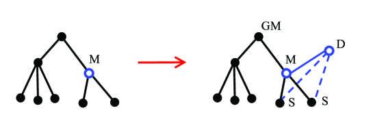
Figure 1: (Color online) Illustration of the corded ND model. A random node, referred to as a mother node, M (empty circle) is selected for duplication. The newly created daughter node, D (empty circle) forms a deterministic edge (solid line) to the mother node, and with probability $p$ it forms a probabilistic edge (dashed line) to each one of the neighbors of M. In this example, D forms links to its two sister nodes, denoted by S, but does not form a link to its grand-mother node, denoted by GM. In this illustration, all the other edges (solid lines) are deterministic edges.

It was shown that for $0<p<1/2$ the corded ND model generates a sparse network, while for $1/2\leq p\leq 1$ the model gives rise to a dense network in which the mean degree increases with the network size Lambiotte2016 ; Bhat2016 . The ND models exhibit the preferential attachment property. This is due to the fact that the probability of a node of degree $k$ to be a neighbor of the randomly selected mother node is proportional to $k$. Therefore, the degrees of the neighbors of the mother node selected at time $t$ are drawn from the distribution

$$\tilde{P}_{t}(K=k)=\frac{kP_{t}(K=k)}{\langle K\rangle_{t}}.$$ (3)

The daughter node forms a link to each one of these nodes with probability $p$. Thus, the probability that the daughter node will form a link to a node of degree $k$ is proportional to $\tilde{P}_{t}(K=k)$. The degree distribution of the corded ND network was studied in Refs. Lambiotte2016 ; Bhat2016 . It was found that for $0<p<1/2$, in the asymptotic limit, the degree distribution of this network follows Eq. (1), where the exponent $\gamma=\gamma(p)$ is given by the non-trivial solution of the equation

$$\gamma=1+p^{-1}-p^{\gamma-2}.$$ (4)

This solution, $\gamma=\gamma(p)$ is a monotonically decreasing function of $p$, in the range of $0<p<1/2$. In the limit of $p\rightarrow 0$, the exponent $\gamma$ diverges like $\gamma(p)\sim 1/p$, while $\gamma(1/2)=2$. In the asymptotic limit, the mean degree is given by

$$\langle K\rangle=\frac{2}{1-2p},$$ (5)

while the second moment of the degree distribution is given by Bhat2016

$$\langle K^{2}\rangle=\left(\frac{2}{1-2p}\right)\left(\frac{3+2p-p^{2}}{1-2p-p^{2}}\right),\ \ \ \ \ 0<p<\sqrt{2}-1.$$ (6)

The sparse network regime can be divided into two parts. For $0<p<\sqrt{2}-1$ the exponent $\gamma(p)>3$, thus in this range the first two moments, $\langle K\rangle$ and $\langle K^{2}\rangle$, are finite. For $\sqrt{2}-1<p<1/2$, the exponent $\gamma$ takes values in the range $2<\gamma(p)<3$, thus in this range the first moment is finite while the second moment diverges. Using Eqs. (5) and (6), it is found that the connective constant

$$\lambda=\frac{\langle K^{2}\rangle-\langle K\rangle}{\langle K\rangle}$$ (7)

of the corded ND network is given by

$$\lambda=\frac{2(1+2p)}{1-2p-p^{2}}.$$ (8)

While in the asymptotic limit the probability $P(K=k)$ may be non-zero for any integer value of $k$, for a finite network of $N$ nodes, it is bounded in the range $1\leq k\leq k_{\rm max}$, where $k_{\rm max}=N-1$.

Node duplication processes capture essential features of empirical networks. For example, an important evolutionary process in genetic regulatory networks is gene duplication, and subsequent mutations of one of the copies Ohno1970 ; Teichmann2004 . As a result, the mutated gene may lose some of its links, and eventually may also form new links. Typically, there is no link between the two copies of the duplicated gene AutoReg . Therefore, the node duplication process resembles the uncorded ND model studied in Refs. Bhan2002 ; Kim2002 ; Chung2003b ; Krapivsky2005 ; Ispolatov2005 ; Ispolatov2005b ; Bebek2006 ; Li2013 . The corded ND model, introduced in Refs. Lambiotte2016 ; Bhat2016 , is suitable for the modeling of acquaintance networks, in which a newcomer who has a friend in a new community becomes acquainted with members of the friend’s social group Toivonen2009 . Unlike the uncorded ND model, the formation of triadic closures is built-in to the dynamics of the corded ND model. This means that once the daughter node forms a link to a neighbor of the mother node, it completes a triangle in which the mother, neighbor and daughter nodes are all connected to each other. The formation of triadic closures is an essential property of the dynamics of social networks where people tend to form a connection to a friend of a friend Granovetter1973 . Therefore, the corded ND model is more suitable for the description of social networks than the uncorded ND model. The corded ND model also describes scientific citation networks Redner1998 ; Redner2005 ; Radicchi2008 , in which the nodes represent papers, while the links represent citations. While acquaintance networks are undirected, citation networks are directed networks, with links pointing from the later (citing) paper to the earlier (cited) paper. It was found that a paper, A, citing an earlier paper, B, often also cites one or several papers, C₁, C₂,$\dots$,C_r, which were cited in B Peterson2010 . The resulting network module consists of $r$ triangles, or triadic closures, which share the AB edge. Since the links of this network are pointing backwards, each one of these triangles can be considered as a feed-backward loop (FBL).

The corded ND model exhibits a unique structure, which is radically different from configuration model networks with the same degree distribution. Unlike the configuration model network Molloy1995 ; Newman2001 , which may include small, isolated clusters, the corded ND network consists of a single connected component. Therefore, unlike the configuration model, it does not exhibit a percolation transition. Also, while the configuration model network exhibits a local tree-like structure, the ND network includes a large number of triangles and other short cycles even in the dilute case of $0<p<1/2$ Lambiotte2016 ; Bhat2016 . Interestingly, many empirical networks exhibit a high abundance of triangles, both in undirected networks Newman2001b and in directed networks, where most triangles form FFLs, while triangular feedback loops are rare Milo2002 ; Alon2006 .

In the special case of $p=0$, the corded ND network is a tree, which consists only of the mother-daughter edges. This tree turns out to form a backbone for the corded ND network at $p>0$, and is thus refereed to as the backbone tree. Once a mother node is selected for duplication, the mother-daughter edge is added deterministically. Therefore, the edges of the backbone tree are called deterministic edges. The other edges, which exist only for $p>0$, are called probabilistic edges. In the limit of $p=0$, where the corded ND network is a tree, the shortest path between any pair of nodes is unique. In fact, on a tree structure the shortest path is the only path between any pair of nodes. Since the path which resides on the backbone tree consists only of deterministic edges, it is referred to as the deterministic path. For $p>0$ the tree is decorated by probabilistic edges. These edges may give rise to alternate paths between any pair of nodes, in addition to the deterministic path which fully resides on the backbone tree. An alternate path may consist of probabilistic edges alone, or from a combination of probabilistic and deterministic edges. In case that the deterministic path between a pair of nodes is shorter than all the alternate paths, it remains the unique shortest path. When the shortest among the alternate paths between a pair of nodes are of the same length as the deterministic path, the shortest path becomes degenerate. Alternate paths may also be shorter than the deterministic path, in which case they become the shortest paths.

In this paper we present analytical results for the DSPL of the corded ND model. Focusing on the sparse network regime of $0<p<1/2$, we derive a master equation for the time evolution of the probabilities $P_{t}(L=\ell)$, where $\ell=1,2,\dots$ is the distance between a pair of nodes and $t$ is the time. The derivation of the master equation requires information on the structure of the backbone tree and on the degeneracies of the shortest paths. Solving the master equation we obtain an expression for $P_{t}(L=\ell)$, which consists of two convolution-like sums. The first sum emanates from the DSPL of the seed network, $P_{0}(L=\ell)$, while the second sum involves a discrete exponential function. We calculate the mean distance, $\langle L\rangle_{t}$, and the diameter, $\Delta_{t}$, and show that in the long-time limit they scale like $\ln t$, namely the corded ND network is a small-world network Milgram1967 ; Watts1998 ; Chung2002 ; Chung2003 . Interestingly, this behavior differs from other scale-free networks which are ultrasmall, namely their mean distance follows $\langle L\rangle_{t}\sim\ln\ln t$ Cohen2003 .

The paper is organized as follows. In Sec. II we present the corded ND model. In Sec. III we analyze the backbone tree, consisting of the mother-daughter edges. In Sec. IV we consider the degeneracies of the shortest paths in the corded ND network. Using the results of sections III and IV we derive, in Sec. V, a master equation for the time evolution of the DSPL and solve it analytically. In Sec. VI we study properties of the DSPL. The mean distance is studied in Sec. VII, the diameter is evaluated in Sec. VIII and the variance of the DSPL is obtained in Sec. IX. The results are discussed in Sec. X and summarized in Sec. XI.

II The corded node duplication model

Consider the corded ND model introduced in Refs. Lambiotte2016 ; Bhat2016 . At each time step, a random node, referred to as the mother node, is selected for duplication. The daughter node is added to the network, forming a link to the mother node and with probability $p$ to each neighbor of the mother node Lambiotte2016 ; Bhat2016 . The growth process starts from an initial seed network of $N_{0}=s$ nodes. Thus, the network size after $t$ time steps is $N_{t}=t+s$.

In Fig. 2 we present two instances of the corded ND network, of size $N_{t}=50$, which were formed around the same backbone tree. Both networks were grown from a seed of size $s=2$, with $p=0.1$ [Fig. 2(a)] and $p=0.4$ [Fig. 2(b)]. Each network instance includes $N_{t}-1=49$ deterministic edges (solid lines). The network of Fig. 2(b) is denser and includes $21$ probabilistic edges (dashed lines), compared to $3$ probabilistic edges in Fig. 2(a).

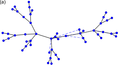
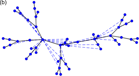
Figure 2: (Color online) Two instances of corded ND networks of size $N=50$, with $p=0.1$ (a) and $p=0.4$ (b). For the sake of comparison, both instances are formed around the same backbone tree (solid lines). The probabilistic edges (dashed lines) essentially decorate the tree. Upon formation, a probabilistic edge shortens the distance between its two ends from $L=2$ to $L=1$, forming a triangle. Increasing $p$ makes the network denser.

The corded ND model exhibits many interesting properties. Since the mother node at time $t$ is selected randomly from all the $N_{t}$ nodes in the network, its degree is effectively drawn from the degree distribution $P_{t}(K=k)$. The mother node gains a link to the daughter node, thus its degree increases by 1. By construction, the degree of the daughter node cannot exceed the degree of the mother node. In case that all the links are duplicated, the degree of the daughter node is equal to the degree of the mother node, while in case that none of them is duplicated the degree of the daughter node is 1.

In order to obtain a connected network, it is required that the seed network will consist of a single connected component. The size of the seed network is denoted by $s$ and its degree distribution is $P_{0}(K=k)$. The mean degree of the seed network is denoted by $\langle K\rangle_{0}$. The DSPL of the seed network is denoted by $P_{0}(L=\ell)$ and the mean distance is denoted by $\langle L\rangle_{0}$. The DSPL and the mean degree are related by $P_{0}(L=1)=\langle K\rangle_{0}/(s-1)$. The probability $P_{0}(L=\ell)$ may take non-zero values for $\ell=1,2,\dots,\Delta_{0}$, where $\Delta_{0}$ is the diameter of the seed network, while $P_{0}(L=\ell)=0$ for $\ell\geq\Delta_{0}+1$. For seed networks of $s$ nodes, $\Delta_{0}$ may take values in the range $1\leq\Delta_{0}\leq s-1$.

The most convenient choice of a seed network is a complete graph of $s$ nodes. In this case, the degree distribution of the seed network is $P_{0}(K=k)=\delta_{k,s-1}$. The DSPL of the seed network is $P_{0}(L=\ell)=\delta_{\ell,1}$, where $\delta_{i,j}$ is the Kronecker delta, and its diameter is $\Delta_{0}=1$. To avoid memory effects, which slow down the convergence to the asymptotic structure, it is often convenient to use a seed network which consists of a single node, namely $s=1$. In this case the degree distribution of the seed network is given by $P_{0}(K=k)=\delta_{k,0}$, while its DSPL is not defined. However, the DSPL becomes well defined at time $t=1$, when the network consists of a pair of connected nodes, whose degree distribution is given by $P_{1}(K=k)=\delta_{k,1}$, its DSPL is $P_{1}(L=\ell)=\delta_{\ell,1}$ and its diameter is $\Delta_{1}=1$. Another interesting choice for the seed network is a linear chain of $s$ nodes. In this case, the initial degree distribution is $P_{0}(K=k)=(2/s)\delta_{k,1}+(1-2/s)\delta_{k,2}$, and the initial DSPL is

$$P_{0}(L=\ell)=\frac{s-\ell}{\binom{s}{2}},$$ (9)

for $\ell=1,2,\dots,s-1$. This choice captures the largest possible diameter in a seed network of $s$ nodes, namely $\Delta_{0}=s-1$.

III The backbone tree

The mother-daughter links in the corded ND network form a random tree structure, which serves as a backbone tree for the resulting network. The backbone tree is a random recursive tree Smythe1995 ; Drmota1997 ; Drmota2005 . To study its properties, one can take the limit of $p=0$, in which the corded ND network is reduced to the backbone tree. The degree distribution of the backbone tree, denoted by $P^{\rm B}_{t}(K=k)$, evolves in time according to

$$P^{\rm B}_{t+1}(K=k)=\frac{1}{N_{t}+1}\left[(N_{t}-1)P^{\rm B}_{t}(K=k)+P^{\rm B}_{t}(K=k-1)+\delta_{k,1}\right].$$ (10)

The second term on the right hand side accounts for the degree of the mother node, which increases by 1 due to the link to the daughter node. The third term accouts for the degree of the daughter node (which is $K=1$), while the first term accounts for all the other nodes in the network. Subtracting $P^{\rm B}_{t}(K=k)$ from both sides of Eq. (10) and replacing the difference on the left hand side by a time derivative we obtain

$$\frac{d}{dt}P^{\rm B}_{t}(K=k)=\frac{1}{N_{t}+1}\left[-2P^{\rm B}_{t}(K=k)+P^{\rm B}_{t}(K=k-1)+\delta_{k,1}\right].$$ (11)

In the long time limit, the degree distribution is expected to reach a steady state, in which the time derivative vanishes. The steady state solution of Eq. (11) is given by

$$P^{\rm B}(K=k)=\frac{1}{2^{k}}.$$ (12)

The corresponding tail distribution is given by $P^{\rm B}(K>k)=1/2^{k}$. Note that the degree distribution of the backbone tree, given by Eq. (12), is a discrete exponential distribution. It is very different from the degree distribution of the full corded ND network, which is a power-law distribution. Eq. (12) captures important properties of the network. In particular, it shows that half of the nodes in the backbone tree are leaf nodes, which have only one link. One fourth of the nodes in the backbone tree have two links, namely they lie along linear chains with no branching. The remaining nodes are branching points with three or more links.

It is useful to define a conditional degree distribution of the form, $P^{\rm B}(K=k|K>k_{0})$, namely the degree distribution of all the nodes of degree $K>k_{0}$. The conditional degree distribution can be expressed in the form

$$P^{\rm B}(K=k|K>k_{0})=\frac{P^{\rm B}(K=k;K>k_{0})}{P^{\rm B}(K>k_{0})}.$$ (13)

Thus, it is given by

$$P^{\rm B}(K=k|K>k_{0})=\frac{1}{2^{k-k_{0}}}.$$ (14)

For example, this means that nodes which are not leaves (namely of degree $k>1$), are of degree $2$ with probability of $1/2$, are of degree $3$ with probability of $1/4$, and so on.

IV The degeneracy of the shortest paths

Consider a pair of nodes, $i$ and $j$, which are at a distance $L=\ell$ from each other. The shortest path from $i$ to $j$ may be unique or it may be degenerate. In case that the shortest path is degenerate, there are at least two different paths of length $\ell$ from $i$ to $j$ (which may have overlapping segments). In particular, the degenerate paths may differ in the first step, starting from node $i$. Here we focus on the degeneracy of the first step, namely on the number of neighbors of node $i$ which reside on shortest paths from $i$ to $j$. We denote the distribution of degeneracy levels of the first steps of the shortest paths by $P(G=g)$, where $g=1,2,\dots$. In order to calculate the distribution $P(G=g)$ we follow the growth process of the network and consider the shortest path from the newly formed daughter node, D, to a randomly selected target node T. It is important to note that the distances $L_{\rm DT}$ between the daughter node, D, and all the existing nodes, T, in the network are determined upon formation of the node D. This is due to the fact that nodes and edges which will be added later cannot form paths between D and T which are shorter than $L_{\rm DT}$. However, they can form additional paths of length $L_{\rm DT}$, thus increasing the degeneracy of the shortest paths.

Since the shortest paths on the backbone tree are unique, it is expected that for $p\ll 1/2$ the shortest paths between most pairs of nodes will not be degenerate. Moreover, it is expected that degenerate paths will exhibit low degeneracy level, namely the probability $P(G=g)$ will sharply decrease as $g$ is increased. Therefore, we will focus below on the probability of a double degeneracy, $P(G=2)$.

It turns out that there are two growth scenarios which give rise to a double degeneracy of the shortest path from the daughter node, D, to a random target node T. In the first scenario, two probabilistic edges form an alternate path of length $L=2$ between nodes D and GM, which is degenerate with the shortest path which goes along the branch of the backbone tree. In the second scenario, there are two probabilistic edges which form shortcuts between pairs of nodes which are next nearest neighbors on the backbone tree. As a result, they give rise to two degenerate paths of length $L=2$, where each path consists of one deterministic edge and one probabilistic edge.

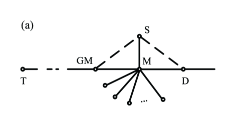
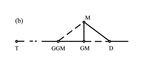
Figure 3: Illustrations of two local network structures which give rise to double degeneracy, $G=2$, in the first step of the shortest path between the daughter node, D, on the right and a target node, T, which resides further down the branch, on the left. In both illustrations, solid lines correspond to deterministic edges, which belongs to the backbone tree, while dashed lines correspond to probabilistic edges. (a) An alternate path of length $L=2$ is formed by probabilistic edges between nodes D and GM, via a sister node, S. This path is degenerate with the primary path which resides fully on the backbone tree. Such structure may form in two distinct sequences of events. One possibility is that S is an older sister which was connected to GM upon formation. When D forms it connects probabilistically to S and completes the alternate path. In the other possibility, S is a younger sister of D, conditioned on D not forming a probabilistic edge to GM upon formation. When S is formed, it connects simultaneously to GM and to D, thus forming the alternate path. (b) In this structure, the distance between D and GGM along the backbone tree is $L=3$, while the shortest paths in the entire network is of length $L=2$. This is achieved by two consecutive probabilistic shortcuts, one from M to GGM (created upon formation of M) and the other from D to GM (created upon formation of D). Note that in this case, the existence of sisters of D (younger or older) makes no difference.

The first scenario is shown in Fig. 3(a). In this scenario, the node D has an older sister, S, which is connected to node GM via a probabilistic edge. In case that D forms a probabilistic edge to S, these two probabilistic edges form an alternate path of length $L=2$ from D to GM. The probability of this scenario is proportional to $p^{2}$. In general, node D may have several sister nodes. The number of such sister nodes is given by $k-2$, where $k$ is the degree of the mother node, M. Therefore, the probability that the path from D to T will be doubly degenerate due to the mechanism of Fig. 3(a) is

$$P(G=2)=\sum_{k=3}^{\infty}{\binom{k-2}{1}}P^{\rm B}(K=k|K>2)p^{2}(1-p^{2})^{k-3},$$ (15)

where $P(K=k|K>2)$ is the conditional degree distribution of the backbone tree, given by Eq. (14). Evaluating the right hand side of Eq. (15) we find that $P(G=2)=p^{2}+O(p^{4})$.

The second scenario is shown in Fig. 3(b). In this case, the mother node, M, is connected not only to its own mother node, GM, but also (with probability $p$) to its grandmother node, referred to as GGM. Upon formation of node D, it may form (with probability $p$) a probabilistic edge to node GM. In such case, there are two degenerate paths from D to GGM. The probability of this scenario is $P(G=g)=p^{2}+O(p^{4})$.

It can be shown that the two scenarios presented above are mutually exclusive, thus the overall probability for the shortest path to be doubly degenerate is

$$P(G=2)=P_{a}(G=2)+P_{b}(G=2)=2p^{2}+O(p^{4}).$$ (16)

A careful analysis shows that the lowest order contribution to $P(G=3)$ is of order $p^{4}$, because at least four probabilistic edges are required. Therefore, to leading order we obtain

$$P(G=1) = 1-2p^{2}+O(p^{4})$$

$$P(G=2) = 2p^{2}+O(p^{4})$$

$$P(G=3) = O(p^{4}).$$ (17)

Truncating the distribution $P(G=g)$ at a degree $g=g_{\rm max}$, its moments can be expressed by

$$\langle G^{n}\rangle=\sum_{g=1}^{g_{\rm max}}g^{n}P(G=g).$$ (18)

Taking $g_{\rm max}=2$, we find that $\langle G\rangle=1+2p^{2}$ and $\langle G^{2}\rangle=1+6p^{2}$.

V The distribution of shortest path lengths

Consider an instance of the corded ND network with a distance matrix $L_{t}$ of dimensions $N_{t}\times N_{t}$, where $L_{t}(i,j)=\ell_{ij}(t)$ is the distance betwen nodes $i$ and $j$ at time $t$. A splendid property of the corded ND model is that the addition of the daughter node never shortens the distance between any pair of existing nodes, $i$ and $j$, in the network, namely $\ell_{i,j}(t)=\ell_{i,j}$ is fixed. Thus, the distance matrix $L_{t+1}$ consists of the matrix $L_{t}$, with the addition a row (and a column) which account for the distances between the daughter node, D, and the rest of the network. This property enables us to express the DSPL at time $t+1$ as a superposition of the DSPL at time $t$ and the DSPL between the daughter node, D, and the rest of the network.

Choosing a random node, $i$, one can describe the shell structure around such a node by the distance distribution

$$P_{t}(L=\ell)=\frac{N_{t}(L=\ell)}{N_{t}-1},$$ (19)

where $N_{t}(L=\ell)$ is the number of nodes in the shell at distance $\ell$ from node $i$. At each time step, $t$, a random node M, referred to as a mother node, is chosen for duplication. The new, daughter node, D, is then connected to the mother node, and with probability $p$ to each one of its neighbors. The shell structure around the daughter node is closely related to that of the mother node. Among the neighbors of the mother node, those of the neighbors for which the link to M is copied, end up at distance $L=1$ from D. Those neighbors of M for which the link to M is not copied end up at distance $L=2$ from D. Therefore, the first shell around the daughter node is given by

$$P_{t}^{\rm D}(L=1)=pP_{t}^{\rm M}(L=1)+\frac{1}{N_{t}-1},$$ (20)

where $P_{t}^{\rm M}(L=\ell)$ is the distance distribution around the mother node. Thus, nodes which are at distance $L=\ell$ from the mother node, may end up either at distance $L=\ell$ or at distance $L=\ell+1$ from the daughter node. To exemplify this property, consider a target node T at distance $L=\ell$ from the mother node, M. A shortest path from M to T consists of a set of nodes ${\rm M},r_{1},r_{2},\dots,r_{\ell-1},{\rm T}$ in which subsequent nodes are connected. In the case that the edge between M and $r_{1}$ is copied, node T ends up at a distance $L=\ell$ from D, while in case it is not copied node T ends up at a distance $L=\ell+1$ from D. In the case that there is a single shortest path from M to T, the former scenario would occur with probability $p$ while the latter scenario would occur with probability $1-p$, namely

$$P_{t}^{\rm D}(L=\ell)=pP_{t}^{\rm M}(L=\ell)+(1-p)P_{t}^{\rm M}(L=\ell-1),$$ (21)

where $\ell\geq 2$. However, since the shortest path from M to T may be degenerate, the calculation of $P_{t}^{\rm D}(L=\ell)$ requires a more careful attention. We express the DSPL between the daughter node, D, and the rest of the network in the form

$$P_{t}^{\rm D}(L=\ell)=\eta P_{t}^{\rm M}(L=\ell)+(1-\eta)P_{t}^{\rm M}(L=\ell-1).$$ (22)

where $\ell\geq 2$ and $0<\eta<1$. The assumption made here is that $\eta=\eta(p)$ does not depend on the path length $L$.

In order to evaluate the parameter $\eta$, consider a random target node, T, which is at distance $\ell$ from the mother node, M. In the simplest case, the shortest path, of length $\ell$ from M to T is unique. However, it may be degenerate, in which case there are several paths of length $\ell$ from M to T. Here we are concerned with the degeneracy of the first step along the shortest paths. This degeneracy is given by the number of nearest neighbors of M which reside on at least one shortest path from M to T, and is denoted by $G_{\rm MT}$. Clearly, $G_{\rm MT}\leq k_{\rm M}$, where $k_{\rm M}$ is the degree of the mother node, M.

Consider a pair of nodes M and T, which are at a distance $L=\ell$ from each other, where the degeneracy level of the shortest paths is given by $G_{\rm MT}=g$. In the case that node M is chosen for duplication, if none of the $g$ links of M which reside on shortest paths to T are duplicated, the distance between the daughter node D and T becomes $L=\ell+1$, while in the case that at least one of these $g$ edges is duplicated, the distance is $L=\ell$. Since each link of the mother node, M, is duplicated with probability $p$, the probability that none of them is duplicated is $(1-p)^{g}$. The probability that at least one of these $g$ links will be duplicated is $1-(1-p)^{g}$. In order to account for the probabilistic nature of the degeneracy, we denote the probability that the first step in the shortest path between random nodes M and T is $g$-fold degenerate by $P_{t}(G=g)$. Thus, the probability, $\eta=\eta(p)$, that at least one of the $g$ neighbors of the mother node, M, which reside along shortest paths to T are connected to the daughter node can be expressed by

$$1-\eta=\sum_{g=1}^{\infty}(1-p)^{g}P(G=g),$$ (23)

or more concisely by

$$1-\eta=\left\langle(1-p)^{G}\right\rangle.$$ (24)

In fact, Eq. (23) can also be expressed in the form

$$1-\eta=F(1-p),$$ (25)

where

$$F(x)=\sum_{g=1}^{\infty}x^{g}P(G=g)$$ (26)

is the generating function of $P(G=g)$.

For simplicity we assume that the distribution $P(G_{\rm MT}=g)$ does not depend on $L_{\rm MT}$, except for the case of $L_{\rm MT}=1$, in which $P(G=g)=\delta_{g,1}$. If this assumption holds, it guarantees that the assumption made above that $\eta$ is independent of $L_{\rm MT}$ is valid.

Using the binomial expansion of $(1-p)^{g}$ in Eq. (23), it can be expressed in the form

$$\eta=-\sum_{n=1}^{\infty}(-1)^{n}B_{n}p^{n},$$ (27)

where

$$B_{n}=\sum_{g=n}^{\infty}{\binom{g}{n}}P(G=g)$$ (28)

is the $n$th binomial moment of $P(G=g)$. The first two terms in this expansion are $\eta=B_{1}p-B_{2}p^{2}$, where $B_{1}=\langle G\rangle$ and $B_{2}=(\langle G^{2}\rangle-\langle G\rangle)/2$. Taking the first term in Eq. (27), where $B_{1}=1+2p^{2}$, we obtain

$$\eta=p+2p^{3}+O(p^{4}).$$ (29)

While paths of length $L=1$ are non-degenerate, for simplicity we replace the parameter $p$ by $\eta$ also in the equation for $P_{t}^{\rm D}(L=1)$. Since $p$ and $\eta$ differ from each other only in order $p^{3}$, while $P_{t}(L=1)$ is quickly reduced to order $1/N_{t}$, the error introduced by this approximation is negligible.

Assuming that the mother node, M, is a typical node, we replace the distribution $P_{t}^{\rm M}(L=\ell)$ by $P_{t}(L=\ell)$. As a result, Eqs. (20) and (22) are replaced by

$$P_{t}^{\rm D}(L=1)=\eta P_{t}(L=1)+\frac{1}{N_{t}-1},$$ (30)

and

$$P_{t}^{\rm D}(L=\ell)=\eta P_{t}(L=\ell)+(1-\eta)P_{t}(L=\ell-1),$$ (31)

respectively, where $\ell\geq 2$. After the node duplication step is completed, the DSPL at time $t+1$ is given by

$$P_{t+1}(L=\ell)=\frac{N_{t}-1}{N_{t}+1}P_{t}(L=\ell)+\frac{2}{N_{t}+1}P_{t}^{\rm D}(L=\ell)-\frac{2P_{t}(L=\ell)}{(N_{t}-1)(N_{t}+1)},$$ (32)

where the third term on the right hand side accounts for the dilution of the probability $P_{t+1}(L=\ell)$ due to the addition of the mother-daughter edge to the network. Subtracting $P_{t}(L=\ell)$ from both sides of Eq. (32) and replacing the difference on the left hand side by a time derivative, we obtain

$$\frac{d}{dt}P_{t}(L=\ell)=-\frac{2}{N_{t}+1}P_{t}(L=\ell)+\frac{2}{N_{t}+1}P_{t}^{\rm D}(L=\ell)-\frac{2P_{t}(L=\ell)}{(N_{t}-1)(N_{t}+1)},$$ (33)

where $N_{t}=t+s$. Plugging in the expressions for $P_{t}^{\rm D}(L=\ell)$ from Eqs. (30) and (31) we obtain

$$\frac{d}{dt}P_{t}(L=1) = -2\left(\frac{1-\eta}{t+s+1}\right)P_{t}(L=1)+\frac{2\left[1-P_{t}(L=1)\right]}{(t+s-1)(t+s+1)},$$ (34)

and

$$\frac{d}{dt}P_{t}(L=\ell) = -2\left(\frac{1-\eta}{t+s+1}\right)P_{t}(L=\ell)+2\left(\frac{1-\eta}{t+s+1}\right)P_{t}(L=\ell-1)$$ (35)

$$- \frac{2}{(t+s-1)(t+s+1)}P_{t}(L=\ell),$$

where $\ell\geq 2$. The solution of Eqs. (34) and (35), for $s\geq 2$, is given by

$$P_{t}(L=1) = \frac{s-1}{t+s-1}\left(\frac{s+1}{t+s+1}\right)^{1-2\eta}P_{0}(L=1)$$ (36)

$$+ \frac{2}{(1-2\eta)(t+s-1)}\left[1-\left(\frac{s+1}{t+s+1}\right)^{1-2\eta}\right],$$

and

$$P_{t}(L=\ell) = \left(\frac{s-1}{s+1}\right)\left(\frac{t+s+1}{t+s-1}\right)\sum_{\ell^{\prime}=1}^{\rm{min}\{\ell,\Delta_{0}\}}\frac{e^{-c_{t}}c_{t}^{\ell-\ell^{\prime}}}{(\ell-\ell^{\prime})!}P_{0}(L=\ell^{\prime})$$ (37)

$$+ \frac{1}{(1-\eta)(s+1)}\left(\frac{t+s+1}{t+s-1}\right)\sum_{\ell^{\prime}=0}^{\infty}\frac{e^{-c_{t}}c_{t}^{\ell+\ell^{\prime}}}{(\ell+\ell^{\prime})!}e^{-\mu\ell^{\prime}},$$

for $\ell\geq 2$, where

$$c_{t}=2(1-\eta)\ln\left(\frac{t+s+1}{s+1}\right),$$ (38)

and

$$\mu=\ln\left(\frac{2-2\eta}{1-2\eta}\right).$$ (39)

The parameter $\eta$ is given by Eq. (23). Note that for $\eta=1/2$, the exponent $e^{-\mu}=0$, thus all the terms in the second sum of Eq. (37) vanish except for the term $\ell^{\prime}=0$. For $1/2<\eta<1$ it is convenient to replace the term $e^{-\mu\ell^{\prime}}$ by

$$\left(\frac{1-2\eta}{2-2\eta}\right)^{\ell^{\prime}}=(-1)^{\ell^{\prime}}\left|\frac{1-2\eta}{2-2\eta}\right|^{\ell^{\prime}}.$$ (40)

Thus, for $\eta>1/2$ the second sum in Eq. (37) consists of positive terms for even values of $\ell^{\prime}$ and negative terms for odd values of $\ell^{\prime}$.

Eqs. (36) and (37) provide a closed form expression for the DSPL of the corded ND network at time $t$ for any size and degree distribution of the seed network. The first term in each of these equations accounts for the effect of the DSPL of the seed network, $P_{0}(L=\ell)$, while the second term does not depend on the initial DSPL. The first sum in Eq. (37) is a convolution between the DSPL of the seed network and a Poisson distribution. The second sum is a convolution between an exponential function and a Poisson distribution.

Eq. (37) can also be written in the form

$$P_{t}(L=\ell) = \left(\frac{s-1}{s+1}\right)\left(\frac{t+s+1}{t+s-1}\right)\sum_{\ell^{\prime}=1}^{\rm{min}\{\ell,\Delta_{0}\}}\frac{e^{-c_{t}}c_{t}^{\ell-\ell^{\prime}}}{(\ell-\ell^{\prime})!}P_{0}(L=\ell^{\prime})$$ (41)

$$+ \frac{1}{(1-\eta)(s+1)}\left(\frac{t+s+1}{t+s-1}\right)e^{-c_{t}(1-e^{-\mu})}e^{\mu\ell}\left[1-\frac{\Gamma(\ell,c_{t}e^{-\mu})}{\Gamma(\ell)}\right],$$

where $\Gamma(x)$ is the Gamma function and $\Gamma(x,y)$ is the incomplete Gamma function.

In Fig. 4 we present the parameter $\eta$ as a function of $p$. The theoretical results (solid line), obtained from Eq. (29), are found to be in good agreement with computer simulations (circles). The value of $\eta$ extracted from the simulations is the value which provides the best fit to the DSPL of Eq. (37), when incorporated in Eq. (22). Since $\eta=\eta(p)$ increases faster than linearly with $p$, there is a point $0<p^{\ast}<1/2$, for which $\eta(p^{\ast})=1/2$. Solving Eq. (29) for $\eta(p^{\ast})=1/2$ we find that $p^{\ast}=[(9+\sqrt{105})/72]^{1/3}-[3(9+\sqrt{105})]^{-1/3}\simeq 0.385$.

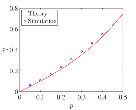
Figure 4: (Color online) The parameter $\eta$ as a function of the probability $p$. This parameter represents the probability that the distance between the daughter node, D, and a random target node, T, is equal to the distance between the mother node, M, and T, namely $\eta=P(L_{DT}=L_{MT})$. Hence, the probability that $L_{DT}=L_{MT}+1$ is given by $1-\eta$. The theoretical results (solid line), obtained from Eq. (29) are found to be in good agreement with the simulation results (circles). For small values of $p$, where the shortest paths are most likely to be unique, $\eta$ is equal to $p$. As $p$ is increased, the shortest paths become degenerate. As a result, $\eta$ acquires a nonlinear dependence on $p$, making it larger than $p$.

In Fig. 5 we present the DSPL, denoted by $P_{t}(L=\ell)$ vs. $\ell$ for an ensemble of corded ND networks of size $N_{t}=10^{4}$, grown from a seed network of size $s=2$, with $p=0.1,0.2,0.3$ and $0.4$. For small values of $p$, the analytical results (solid lines) are in very good agreement with the simulation results (circles). As $p$ is increased, the analytical results become shifted to the right compared to the simulation results. The simulation data was averaged over 100 network instances.

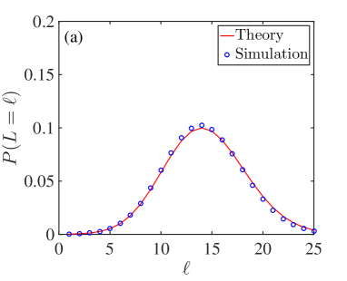
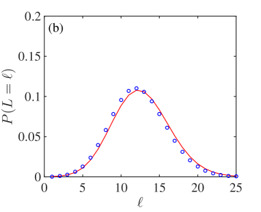
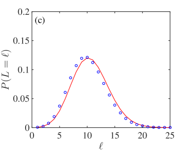
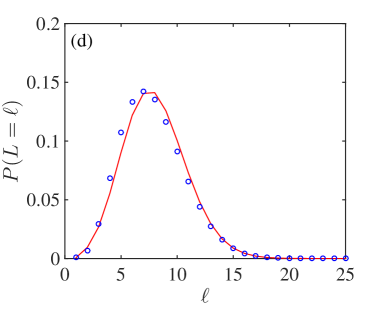
Figure 5: (Color online) The DSPL of the corded ND network of $N_{t}=10^{4}$ nodes with (a) $p=0.1$, (b) $p=0.2$, (c) $p=0.3$, and (d) $p=0.4$. The theoretical results (solid lines), obtained from Eqs. (36) and (37) are found to be in good agreement with the results of computer simulations (circles), obtained by averaging over $100$ instances. As $p$ is increased, the distances become shorter and the DSPL becomes narrower, consistent with Eqs. (58) and (74). The agreement is better for smaller values of $p$. In fact, Eqs. (36) and (37) are exact, while the deviation from the simulation results are due to the underestimate of $\eta$, as can be seen in Fig. 4.

VI Properties of the DSPL

The first sum in Eq. (37) accounts for paths which emerge from repeated duplication of nodes and edges along paths of the seed network. It can be noted that the probability $P_{t}(L=\ell)$ is affected only by the initial probabilities $P_{0}(L=\ell^{\prime})$ for which $\ell^{\prime}\leq\ell$. This is due to the fact that the distance from a daughter node to any other node in the network is equal or larger by $1$ than the distance from the mother node. The second sum accounts for repeated duplication of nodes and edges along new paths that emerge beyond the seed network. The exponential function accounts for the backbone tree structure which emerges from the edges connecting the mother and daughter nodes. The Poisson distribution accounts for the probabilistic connections to the neighbors of the mother node. Both sums in Eq. (37) involve the same Poisson distribution, $P(m)=e^{-c_{t}}c_{t}^{m}/m!$, whose mean, $c_{t}$ is given by Eq. (38). The first sum runs over terms in the range $m=\ell-1,\ell-2,\dots,{\rm max}\{0,\ell-s+1\}$, while the second sum runs over terms in the range $m=\ell,\ell+1,\dots,\infty$.

Below we consider some special cases and limits in which the expression for $P_{t}(L=\ell)$ can be simplified. In particular, we study specific choices of the seed network, such as a complete graph of $s$ nodes, and the special case of a single node, in which $s=1$. We also consider specific values of the parameter $p$, such as $p=0$, in which the corded ND network is reduced to the backbone tree. Another special case is the value of $p$ for which $\eta(p)=1/2$. In this case, the parameter $\mu$ diverges. As a result, the exponentials, $e^{-\mu\ell^{\prime}}$, in the second sum in Eq. (37) vanish, except for the term with $\ell^{\prime}=0$, thus the sum is reduced to a single term.

A convenient choice for the seed network is a complete graph of $s\geq 2$ nodes. In this case the initial DSPL is given by $P_{0}(L=1)=1$ and $P_{0}(L\geq 2)=0$. The expression for the DSPL at time $t$ is simplified to

$$P_{t}(L=1)=\frac{s-1}{t+s-1}\left(\frac{s+1}{t+s+1}\right)^{1-2\eta}+\frac{2}{(1-2\eta)(t+s-1)}\left[1-\left(\frac{s+1}{t+s+1}\right)^{1-2\eta}\right],$$ (42)

and

$$P_{t}(L=\ell)=\left(\frac{t+s+1}{t+s-1}\right)\left[\left(\frac{s-1}{s+1}\right)\frac{e^{-c_{t}}c_{t}^{\ell-1}}{(\ell-1)!}+\frac{1}{(1-\eta)(s+1)}\sum_{\ell^{\prime}=0}^{\infty}\frac{e^{-c_{t}}c_{t}^{\ell+\ell^{\prime}}}{(\ell+\ell^{\prime})!}e^{-\mu\ell^{\prime}}\right],$$ (43)

for $\ell\geq 2$, where $c_{t}$ is given by Eq. (38) and $\mu$ is given by Eq. (39).

In case that the seed network consists of a single node, $s=1$, the probability $P_{0}(L=\ell)=0$ is not defined. However, after one time step, at $t=1$, the network consists of a pair of connected nodes, where $P_{1}(L=1)=1$ and $P_{1}(L\geq 2)=0$. Thus, the ensemble of networks obtained at time $t$ for a seed network of size $s=1$ is identical to the network ensemble obtained at time $t-1$ from a seed network of size $s=2$, namely $P_{t}(L=\ell|s=1)=P_{t-1}(L=\ell|s=2)$. The DSPL of the resulting ND network, for $t\geq 1$, takes the form

$$P_{t}(L=1)=-\left(\frac{1+2\eta}{1-2\eta}\right)\left(\frac{3}{t+2}\right)^{1-2\eta}\frac{1}{t}+\left(\frac{2}{1-2\eta}\right)\frac{1}{t},$$ (44)

and

$$P_{t}(L=\ell)=\frac{1}{3}\left(\frac{t+2}{t}\right)\left[\frac{e^{-c_{t}}c_{t}^{\ell-1}}{(\ell-1)!}+\frac{1}{1-\eta}\sum_{\ell^{\prime}=0}^{\infty}\frac{e^{-c_{t}}c_{t}^{\ell+\ell^{\prime}}}{(\ell+\ell^{\prime})!}e^{-\mu\ell^{\prime}}\right],$$ (45)

for $\ell\geq 2$, where $c_{t}$ is given by Eq. (38) and $\mu$ is given by Eq. (39).

In case that the parameter $p=0$, each daughter node is formed with a single edge connecting it to its mother node. In this case, the corded ND network is reduced to the backbone tree. Upon formation of the daughter node, all the paths from it to existing nodes go through the mother node. They are thus longer by $1$ than the paths starting from the mother node. In this case, Eq. (36) is simplified to

$$P_{t}(L=1)=\frac{(s-1)(s+1)}{(t+s-1)(t+s+1)}P_{0}(L=1)+\frac{2t}{(t+s-1)(t+s+1)}.$$ (46)

In case that $p=0$ the parameters $\eta$ and $\mu$ take the values $\eta=0$ and $\mu=\ln 2$. Thus, Eq. (41) is reduced to

$$P_{t}(L=\ell) = \left(\frac{s-1}{s+1}\right)\left(\frac{t+s+1}{t+s-1}\right)\sum_{\ell^{\prime}=1}^{\rm{min}\{\ell,\Delta_{0}\}}\frac{e^{-c_{t}}c_{t}^{\ell-\ell^{\prime}}}{(\ell-\ell^{\prime})!}P_{0}(L=\ell^{\prime})$$ (47)

$$+ \left(\frac{t+s+1}{t+s-1}\right)\left(\frac{e^{-c_{t}/2}2^{\ell}}{s+1}\right)\left[1-\frac{\Gamma(\ell,c_{t}/2)}{\Gamma(\ell)}\right],$$

where

$$c_{t}=2\ln\left(\frac{t+s+1}{s+1}\right).$$ (48)

Another interesting case appears for $p=p^{\ast}$, where $\eta=\eta(p^{\ast})=1/2$. In this case Eq. (37) is reduced to

$$P_{t}(L=\ell)=\left(\frac{t+s+1}{t+s-1}\right)\left[\left(\frac{s-1}{s+1}\right)\sum_{\ell^{\prime}=1}^{{\rm min}\{\ell,\Delta_{0}\}}\frac{e^{-c_{t}}c_{t}^{\ell-\ell^{\prime}}}{(\ell-\ell^{\prime})!}P_{0}(L=\ell^{\prime})+\frac{2}{s+1}\frac{e^{-c_{t}}c_{t}^{\ell}}{\ell!}\right].$$ (49)

For the special case in which the seed network is a complete graph, Eq. (49) is further redued to the form

$$P_{t}(L=\ell)=\left(\frac{t+s+1}{t+s-1}\right)\left[\left(\frac{s-1}{s+1}\right)\frac{e^{-c_{t}}c_{t}^{\ell-1}}{(\ell-1)!}+\frac{2}{s+1}\frac{e^{-c_{t}}c_{t}^{\ell}}{\ell!}\right],$$ (50)

where $\ell\geq 2$.

VII The mean distance

The mean distance between a random pair of nodes in the corded ND network is given by

$$\langle L\rangle_{t}=\sum_{\ell=1}^{\infty}\ell P_{t}(L=\ell).$$ (51)

Taking the time derivative of Eq. (51) and plugging in the expressions for $dP_{t}(L=1)/dt$ from Eq. (34) and for $dP_{t}(L=\ell)/dt$ from Eq. (35) we obtain

$$\frac{d}{dt}\langle L\rangle_{t} = \frac{2(\eta-1)(t+s)-2\eta}{(t+s-1)(t+s+1)}\sum_{\ell=1}^{\infty}\ell P_{t}(L=\ell)+\frac{2(1-\eta)}{t+s+1}\sum_{\ell=1}^{\infty}(\ell+1)P_{t}(L=\ell)$$ (52)

$$+ \frac{2}{(t+s-1)(t+s+1)}.$$

Rearranging terms we obtain

$$\frac{d}{dt}\langle L\rangle_{t} = -\frac{2}{(t+s-1)(t+s+1)}\langle L\rangle_{t}+\frac{2(1-\eta)}{t+s+1}+\frac{2}{(t+s-1)(t+s+1)}.$$ (53)

Solving Eq. (53) we obtain

$$\langle L\rangle_{t} = 2(1-\eta)\left(\frac{t+s+1}{t+s-1}\right)\ln\left(\frac{t+s+1}{s+1}\right)+\left(\frac{s-1}{s+1}\right)\left(\frac{t+s+1}{t+s-1}\right)\langle L\rangle_{0}$$ (54)

$$- \left(\frac{2}{s+1}\right)\left(\frac{1}{1-2\eta}\right)\left(\frac{t}{t+s-1}\right).$$

In the long time limit, Eq. (54) is reduced to

$$\langle L\rangle_{t}=2(1-\eta)\ln\left(\frac{t+s+1}{s+1}\right)+C_{1}+C_{2},$$ (55)

where

$$C_{1}=\left(\frac{s-1}{s+1}\right)\langle L\rangle_{0}$$ (56)

and

$$C_{2}=-\left(\frac{2}{s+1}\right)\left[\frac{1-4\eta(1-\eta)}{1-2\eta}\right].$$ (57)

The term $C_{1}$ accounts for the effect of the DSPL of the seed network on $\langle L\rangle_{t}$. The term $C_{2}$ is a negative term which depends on $p$ and $s$. For $0<p<p^{\ast}$ (where $0<\eta<1/2$), it is bounded in the range $-2/(s+1)<C_{2}<0$. For $p>p^{\ast}$ it becomes smaller than $-2/(s+1)$, thus reducing the mean distance $\langle L\rangle_{t}$. In conclusion, in the long time limit the mean distance scales logarithmically with the network size, according to

$$\langle L\rangle_{t}\simeq 2(1-\eta)\ln\left(\frac{t+s+1}{s+1}\right),$$ (58)

which means that the corded ND network is a small-world network.

In Fig. 6 we present the mean distance, $\langle L\rangle_{t}$, as a function of the network size $N_{t}$, for $p=0.1,0.2,0.3$ and $0.4$. The theoretical results, obtained from Eq. (55), where $\eta$ is taken from Eq. (58), are found to be in good agreement with computer simulations (symbols).

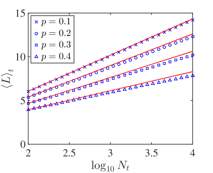
Figure 6: (Color online) The mean shortest path length, $\langle L\rangle_{t}$, of the corded ND network as a function of network size $N_{t}$. The theoretical results (solid lines), obtained from Eq. (58), where $\eta$ is taken from Eq. (29), are generally in good agreement with the simulation results (symbols), confirming the logarithmic dependence on the network size. As $p$ is increased, the mean shortest path length decreases. As in Fig. 5, the deviation between the theory and simulation increases as $p$ is increased, due to the fact that the exact value of $\eta$ is not known. For clarity, we focus on network sizes in the range $10^{2}\leq N_{t}\leq 10^{4}$.

VIII The diameter

Consider an ensemble of corded ND networks of size $N_{t}$. In each instance of the network there are $N_{t}(N_{t}-1)/2$ pairs of nodes and the distances between them follow the distribution $P_{t}(L=\ell)$. The expectation value of the number of pairs of nodes which reside at a distance $L=\ell$ from each other is given by

$$N_{t}(L=\ell)=\frac{N_{t}(N_{t}-1)}{2}P_{t}(L=\ell),$$ (59)

where $N_{t}=t+s$. For sufficiently long times ($t\gg s$), the effect of the seed network is reduced and the DSPL exhibits a well defined peak, above which $P_{t}(L=\ell)$ gradually decreases. As a result, the tail of the DSPL exhibits a distance $\Delta_{t}$, at which $N_{t}(L=\Delta_{t})=1$, which can be considered as the expectation value of the diameter of the network. Below, we use this criterion to evaluate the diameter. For simplicity, we consider the case in which the initial network is a complete graph of $s$ nodes. Note that a network resulting at time $t$ from a seed network of size $s=1$ is equivalent to a network at time $t-1$ with $s=2$. Thus, in the analysis below there is no need to treat the case of $s=1$ separately. Considering the large network limit, and focusing on the large distance tail of the DSPL, it can be expressed by

$$P_{t}(L=\ell)=\left(\frac{s-1}{s+1}\right)\frac{e^{-c_{t}}c_{t}^{\ell-1}}{(\ell-1)!}.$$ (60)

For convenience, we write $c_{t}$ in the form $c_{t}=2(1-\eta)\ln t_{s}$, where

$$t_{s}=\frac{t+s+1}{s+1}$$ (61)

is the network size at time $t+1$, expressed in units of the network size at time $t=1$. Inserting the expression for $c_{t}$ into Eq. (60) and using the Stirling formula we find that

$$N_{t}(L=\ell)=\frac{(s^{2}-1)t_{s}^{2\eta}}{4(1-\eta)\ln t_{s}}\left(\frac{2(1-\eta)e\ln t_{s}}{\ell}\right)^{\ell}.$$ (62)

Inserting $N_{t}(L=\Delta_{t})=1$ in Eq. (62) we obtain

$$\left(\frac{\Delta_{t}}{2e(1-\eta)\ln t_{s}}\right)^{\Delta_{t}}=\frac{(s^{2}-1)t_{s}^{2\eta}}{4(1-\eta)\ln t_{s}}.$$ (63)

Taking a logarithm on both sides and rearranging terms, Eq. (63) can be expressed in the form

$$\left(\frac{\Delta_{t}}{2(1-\eta)e\ln t}\right)\ln\left(\frac{\Delta_{t}}{2(1-\eta)e\ln t}\right)=\frac{4\eta\ln t_{s}-\ln[16\pi(1-\eta)\ln t_{s})]+2\ln\left(s^{2}-1\right)}{4(1-\eta)e\ln t_{s}}.$$ (64)

Applying the Lambert W function Olver2010 on both sides and using the relation $W(ze^{z})=z$, we obtain

$$\ln\left(\frac{\Delta_{t}}{2(1-\eta)e\ln t_{s}}\right)=W\left[\frac{4\eta\ln t_{s}-\ln[16\pi(1-\eta)\ln t_{s}]+2\ln\left(s^{2}-1\right)}{4(1-\eta)e\ln t_{s}}\right],$$ (65)

or

$$\Delta_{t}=2(1-\eta)\exp{\left\{1+W\left[\frac{4\eta\ln t_{s}-\ln\left[16\pi(1-\eta)\ln t_{s}\right]+2\ln\left(s^{2}-1\right)}{4(1-\eta)e\ln t_{s}}\right]\right\}}\ln t_{s}$$ (66)

Taking the long time limit, we can approximate the argument of the $W(x)$ function. The numerator can be replaced by its leading term, which is $2\eta\ln t$, thus

$$\Delta_{t}=2(1-\eta)e^{1+W\left[\frac{\eta}{(1-\eta)e}\right]}\ln t_{s}.$$ (67)

Using again the above mentioned property of the $W(x)$ function, we obtain that the expectation value, $\Delta_{t}$ of the diameter of the corded ND network is given by

$$\Delta_{t}\simeq\frac{2\eta}{W\left[\frac{\eta}{(1-\eta)e}\right]}\ln\left(\frac{t+s+1}{s+1}\right).$$ (68)

The diameter thus scales logarithmically with the network size, namely exhibits the same scaling as the mean distance $\langle L\rangle_{t}$. However, the coefficient is larger than the coefficient of the mean distance. Using Eqs. (58) and (68) we find that

$$\frac{\Delta_{t}}{\langle L\rangle_{t}}=\frac{\eta}{(1-\eta)W\left[\frac{\eta}{(1-\eta)e}\right]}.$$ (69)

In the dilute network limit, where $p\ll 1$, the parameter $\eta$ also satisfies $\eta\ll 1$. Using the leading term in the Taylor expansion of the Lambert W function, given by $W(x)=\sum_{n=1}^{\infty}(-n)^{n-1}x^{n}/n!$, and the relation $\eta=p+2p^{3}$, we obtain

$$\frac{\Delta_{t}}{\langle L\rangle_{t}}=e+p+\frac{2e-1}{2e}p^{2}+O(p^{3}).$$ (70)

Thus, in the limit of $p\ll 1$ the diameter becomes $\Delta_{t}\simeq e\langle L\rangle_{t}$. This is in contrast to the case of configuration model networks, where $\Delta=\langle L\rangle+\delta$, where $\delta$ is an additive constant Bollobas2001 ; Bollobas2007 .

In Fig. 7 we present the diameter of the corded ND network as a function of the network size for $p=0.1,0.2,0.3$ and $0.4$. The analytical results (solid lines), obtained from Eq. (68), where $\eta$ is taken from Eq. (29), confirm that the diameter scales logarithmically with the network size. The analytical results over-estimate the slope compared to the simulation results (symbols). This is due to the fact that the argument used to estimate $\Delta_{t}$ does not account for correlations between the longest distances in a given instance of the network. Thus, the result of Eq. (68) may be considered as an upper bound for the diameter. The simulation data was averaged over $100$ network instances.

Figure 7: (Color online) The diameter $\Delta_{t}$ of the corded ND network as a function of network size, $N_{t}$. The theoretical results (solid lines), obtained from Eq. (68), where $\eta$ is taken from Eq. (29), are found to be in good agreement with the simulation results (symbols). The results confirm the logarithmic dependence of the diameter on the network size. As $p$ is increased, the diameter decreases.

IX The variance of the DSPL

In order to obtain the variance of the DSPL, we need to calculate its second moment, given by $\langle L^{2}\rangle_{t}=\sum_{\ell=1}^{\infty}\ell^{2}P_{t}(L=\ell)$. Taking the time derivative of $\langle L^{2}\rangle_{t}$ and plugging in the expressions for $dP_{t}(L=1)/dt$ from Eq. (34) and for $dP_{t}(L=\ell)/dt$ from Eq. (35) we obtain

$$\frac{d}{dt}\langle L^{2}\rangle_{t} = -\frac{2}{(t+s-1)(t+s+1)}\langle L^{2}\rangle_{t}+\frac{4(1-\eta)}{t+s+1}\langle L\rangle_{t}$$ (71)

$$+ \frac{2(1-\eta)(t+s-1)+2}{(t+s-1)(t+s+1)},$$

where $\langle L\rangle_{t}$ is given by Eq. (55). Keeping only the leading terms we obtain

$$\frac{d}{dt}\langle L^{2}\rangle_{t}=\frac{4(1-\eta)[\ln(t+s+1)+2C_{1}+2C_{2}+1]}{t+s+1}.$$ (72)

Note that as $p$ approaches $1/2$ from below the second term on the right hand side becomes large and cannot be neglected in Eq. (72). The solution of Eq. (72) is

$$\langle L^{2}\rangle_{t}=\langle L^{2}\rangle_{0}+\left[2(1-\eta)\ln\left(\frac{t+s+1}{s+1}\right)\right]^{2}+2(2C_{1}+2C_{2}+1)(1-\eta)\ln\left(\frac{t+s+1}{s+1}\right).$$ (73)

Thus, the variance $\sigma_{t}^{2}=\langle L^{2}\rangle_{t}-\langle L\rangle_{t}^{2}$ is given by

$$\sigma_{t}^{2}=2(1-\eta)\ln\left(\frac{t+s+1}{s+1}\right)+\langle L^{2}\rangle_{0}-(C_{1}+C_{2})^{2}.$$ (74)

In the long time limit, Eq. (74) can be simplified to the form

$$\sigma_{t}^{2}=2(1-\eta)\ln\left(\frac{t+s+1}{s+1}\right)+O(1),$$ (75)

which highlights the logarithmic scaling. Comparing Eqs. (54) and (74) we find that to leading order $\sigma_{t}^{2}=\langle L\rangle_{t}$, which is the result obtained in the case of a Poisson distribution.

In Fig. 8 we present the standard deviation, $\sigma_{t}$, of the DSPL of the corded ND model as a function of network size, $N_{t}$. The analytical results (solid lines), obtained from Eq. (75), where $\eta$ is taken from Eq. (29), are found to be in good agreement with the results of numerical simulations (symbols), thus the logarithmic scaling is confirmed.

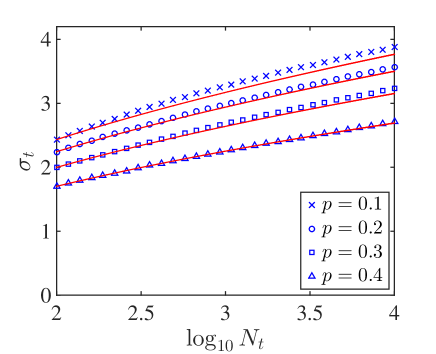
Figure 8: (Color online) The standard deviation of the DSPL, $\sigma_{t}$, as a function of network size, $N_{t}$. The theoretical results (solid lines), obtained from Eq. (75), where $\eta$ is taken from Eq. (29), are found to be in good agreement with the simulation results (symbols).

X Discussion

The mean distance, $\langle L\rangle_{t}$ of the corded ND network was found to scale logarithmically with the network size, $N_{t}$, according to $\langle L\rangle_{t}\simeq 2(1-\eta)\ln N_{t}$, and it is thus a small world network. A similar logarithmic scaling is observed in other random networks such as configuration model networks. However, the pre-factor of the logarithmic term is different. In configuration model networks the mean distance is given by Chung2002 ; Chung2003

$$\langle L\rangle=\frac{1}{\ln\left(\frac{\langle K^{2}\rangle-\langle K\rangle}{\langle K\rangle}\right)}\ln N.$$ (76)

The pre-factor of $\ln N$ is equal to the inverse of the logarithm of the connective constant, which is expressed in terms of the first two moments of the degree distribution. Using Eq. (24), the mean distance of the corded ND network can be expressed in the form

$$\langle L\rangle_{t}\simeq 2\left\langle(1-p)^{G}\right\rangle\ln N_{t}.$$ (77)

Thus, the mean distance in the corded ND network is expressed in terms of the generating function of the distribution of degeneracy levels, $P(G=g)$, unlike the configuration model in which it is given in terms of the first two moments of the degree distribution, $P(K=k)$.

In order to compare the quantitative behaviors of the corded ND network and the configuration model network, we present in Fig. 9 the mean distance, $\langle L\rangle_{t}$, expressed in units of $\ln N_{t}$, of the corded ND network (dashed line) and of the corresponding configuration model network with the same degree distribution (solid line), as a function of $p$. For the corded ND network, this ratio is

$$\frac{\langle L\rangle_{t}}{\ln N_{t}}\simeq 2(1-\eta),$$ (78)

where $\eta$ is given by Eq. (29). For the corresponding configuration model network, it is expressed by

$$\frac{\langle L\rangle}{\ln N}=\frac{1}{\ln\left(\frac{\langle K^{2}\rangle-\langle K\rangle}{\langle K\rangle}\right)},$$ (79)

where $\langle K\rangle$ is given by Eq. (5) and $\langle K^{2}\rangle$ is given by Eq. (6). It is found that for the corded ND network this ratio is of order $1$ for the whole range of sparse networks while in the corresponding configuration model network it decreases as $p$ is increased until it falls sharply to zero at $p=\sqrt{2}-1$.

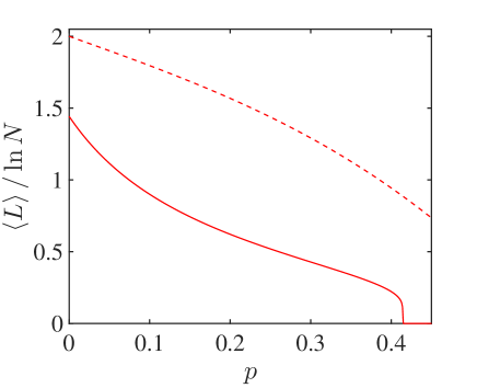
Figure 9: (Color online) The mean distance, $\langle L\rangle=\langle L\rangle_{t}$, expressed in units of $\ln N=\ln N_{t}$, namely $\langle L\rangle/\ln N\simeq 2(1-\eta)$, of the corded ND network as a function of the parameter $p$ (dashed line), and the corresponding ratio, $\langle L\rangle/\ln N=1/\ln[(\langle K^{2}\rangle-\langle K\rangle)/\langle K\rangle]$, for a configuration model network with the same degree distribution (solid line), where $\langle K\rangle$ is given by Eq. (5) and $\langle K^{2}\rangle$ is given by Eq. (6).

We also calculated the diameter, $\Delta_{t}$, of the corded ND network and found that in the long time limit

$$\frac{\Delta_{t}}{\ln N_{t}}\simeq\frac{2\eta}{W\left[\frac{\eta}{(1-\eta)e}\right]},$$ (80)

where $\eta=p+2p^{3}$. For $p\ll 1$, using the Taylor expansion of the Lambert W function we obtain

$$\frac{\Delta_{t}}{\ln N_{t}}=2(1-\eta)\left(e+p+\frac{2e-1}{2e}p^{2}\right)+O(p^{3}).$$ (81)

Thus, in the limit of $p\ll 1$ the diameter becomes $\Delta_{t}\simeq 2e(1-\eta)\ln N_{t}$, namely by a factor of $e$ larger than the mean distance, $\langle L\rangle_{t}$. This is in contrast to the case of configuration model networks, where $\Delta=\langle L\rangle+\delta$, and $\delta$ is an additive constant Bollobas2001 ; Bollobas2007 .

The variance of the DSPL was found to scale like

$$\sigma_{t}^{2}=2(1-\eta)\ln N_{t},$$ (82)

namely the variance scales linearly with the mean distance, which reflects the dominance of the Poisson distribution in the DSPL. Thus, the variance of the DSPL in the corded ND network is much larger than in the corresponding configuration model networks, in which the DSPL tends to be narrow.

It will be interesting to generalize the analysis presented here to the calculation of the DSPL of the uncorded ND network, in which there is no link between the mother and daughter nodes. A useful simplifying property of the corded ND model studied here is that the daughter node is never discarded, namely each randomly selected mother node is actually duplicated. This guarantees that the degree of the mother node selected at time $t$ is drawn from the instantaneous degree distribution, $P_{t}(K=k)$. In the uncorded ND model this is not the case, because the probability that the daughter node will form a link to at least one neighbor of the mother node and thus will be added to the network depends on the degree of the mother node. The conditional probability that the daughter node will be added to the network, given that the mother node is of degree $k$, is $P_{t}({\rm added}|K=k)=1-(1-p)^{k}$. Using Bayes’ theorem, it can by shown that the degree distribution of the mother node under the condition that the daughter node was actually added to the network is

$$P_{t}(K=k|{\rm added})=\frac{1-(1-p)^{k}}{1-G_{t}^{0}(1-p)}P_{t}(K=k),$$ (83)

where $G_{t}^{0}(x)=\sum_{k}x^{k}P_{t}(K=k)$ is the generating function of the degree distribution at time $t$. The fact that $P_{t}(K=k|{\rm added})$ is different from $P_{t}(K=k)$ is expected to make the calculation of the DSPL more difficult, because the mother nodes in this case are not simply random nodes. The DSPL between a node, $i$, of degree $k_{i}$ and the rest of the network depends on $k_{i}$. It will thus require to derive a set of master equations for the conditional DSPLs, $P_{t}(L=\ell|K=k)$, between a random node of degree $k$ and all other nodes in the network.

XI Summary

We have studied a node duplication network model, in which at each time step a random mother node is selected for duplication, referred to as the corded ND model. The daughter node is connected deterministically to the mother node, and is also connected, with probability $p$, to each one of its neighbors. We focused on the regime of dilute networks, obtained for $0<p<1/2$. We derived a master equation for the time evolution of $P_{t}(L=\ell)$. Finding an exact analytical solution of the master equation, we obtained a closed form expression for the DSPL, in which the probability $P_{t}(L=\ell)$ is expressed as a sum of two terms. The first term is a convolution between the DSPL of the seed network, $P_{0}(L=\ell)$, and a Poisson distribution. The second term is a convolution between a discrete exponential function and the Poisson distribution. We calculated the mean distance $\langle L\rangle_{t}$ and showed that in the long time limit it scales like $\langle L\rangle_{t}\simeq 2(1-\eta)\ln N_{t}$, where $N_{t}$ is the network size at time $t$. The mean distance thus scales logarithmically with the network size, which means that the corded ND network is a small world network. Interestingly, this behavior differs from other scale-free networks which are ultrasmall, namely their mean distance follows $\langle L\rangle_{t}\sim\ln\ln N_{t}$ Cohen2003 .

References

- (1) R. Albert and A.L. Barabási, Statistical mechanics of complex networks, Rev. Mod. Phys. 74, 47 (2002).
- (2) G. Caldarelli, Scale free networks: complex webs in nature and technology (Oxford University Press, 2007).
- (3) S. Havlin and R. Cohen, Complex Networks: Structure, Robustness and Function (Cambridge University Press, 2010).
- (4) M.E.J. Newman, Networks: an Introduction (Oxford University Press, 2010).
- (5) E. Estrada, The Structure of Complex Networks: Theory and Applications (Oxford University Press, 2011).
- (6) A. Barrat, M. Barthélemy and A. Vespignani, Dynamical Processes on Complex Networks (Cambridge University Press, 2012).
- (7) R. Milo, S. Shen-Orr, S. Itzkovitz, N. Kashtan, D. Chklovskii and U. Alon, Science 298, 824 (2002).
- (8) U. Alon, An Introduction to Systems Biology: Design Principles of Biological Circuits (Chapman and Hall/CRC, 2006).
- (9) A.-L. Barabasi and R. Albert, Science 286, 509 (1999).
- (10) H. Jeong, B. Tombor, R. Albert, Z.N. Oltvai, and A.-L. Barabási, Nature 407, 651 (2000).
- (11) P. L. Krapivsky, S. Redner and F. Leyvraz, Phys. Rev. Lett. 85, 4629 (2000).
- (12) P.L. Krapivsky and S. Redner, Phys. Rev. E 63, 066123 (2001).
- (13) A. Vázquez, Phys. Rev. E 67, 056104 (2003).
- (14) S. Milgram, Psychology Today 1, 61 (1967).
- (15) D. Watts and S. Strogatz, Nature 393, 440 (1998).
- (16) F. Chung and L. Lu, Proc. Nat. Acad. Sci. USA 99, 15879 (2002)
- (17) F. Chung and L. Lu, Internet Mathematics 1, 91 (2003).
- (18) R. Cohen and S. Havlin, Phys. Rev. Lett. 90, 058701 (2003).
- (19) L. Giot et al., Science 302 1727 (2003).
- (20) A. Maáyan, S.L. Jenkins, S. Neves, A. Hasseldine, E. Grace, B. Dubin-Thaler, N.J. Eungdamrong, G. Weng, P.T. Ram, J.J. Rice, A. Kershenbaum, G.A. Stolovitzky, R.D. Blitzer, R. Iyengar, Science 309, 1078 (2005).
- (21) E.W. Dijkstra, Numerische Mathematik l, 269 (1959).
- (22) D. Delling, P. Sanders, D. Schultes and D. Wagner, Engineering Route Planning Algorithms, in Algorithmics of Large and Complex Networks: Design, Analysis, and Simulation, J. Lerner, D. Wagner, and K.A. Zweig (Eds.), p. 117 (2009).
- (23) R. Pastor-Satorras, C. Castellano, P. Van Mieghem and A. Vespignani, Rev. Mod. Phys. 87, 925 (2015).
- (24) B. Bollobas, Random Graphs, Second Edition (Academic Press, London, 2001).
- (25) R. Durrett, Random Graph Dynamica (Cambridge University Press, Cambridge, 2007).
- (26) A. Fronczak, P. Fronczak, and J.A. Holyst, Phys. Rev. E 70, 056110 (2004).
- (27) M.E.J. Newman, Proc. Natl. Acad. Sci. USA 98, 404 (2001).
- (28) M.E.J. Newman, S.H. Strogatz, and D.J. Watts, Phys. Rev. E 64, 026118 (2001).
- (29) S.N. Dorogotsev, J.F.F. Mendes and A.N. Samukhin, Nuclear Physics B 653, 307 (2003).
- (30) V.D. Blondel, J.-L. Guillaume, J.M. Hendrickx and R.M. Jungers, Phys. Rev. E 76, 066101 (2007).
- (31) R. van der Hofstad, G. Hooghiemstra and D. Znamenski, Electronic Journal of Probability 12, 703 (2007).
- (32) H. van der Esker, R. van der Hofstad and G. Hooghiemstra, J. Stat. Phys. 133, 169 (2008).
- (33) J. Shao, S. V. Buldyrev, R. Cohen, M. Kitsak, S. Havlin, and H. E. Stanley, Europhys. Lett. 84, 48004 (2008).
- (34) J. Shao, S. V. Buldyrev, L. A. Braunstein, S. Havlin, and H. E. Stanley, Phys. Rev. E 80, 036105 (2009).
- (35) E. Katzav, M. Nitzan, D. ben-Avraham, P.L. Krapivsky, R. Kühn, N. Ross and O. Biham, EPL 111, 26006 (2015).
- (36) P. Erdős and A. Rényi, Publ. Math. Debrecen 6, 290 (1959); Publ. Math. Inst. Hungar. Acad. Sci. 5, 17 (1960); Bull. Inst. Internat. Statist 38, 343 (1961).
- (37) M. Nitzan, E. Katzav, R. Kühn and O. Biham, Phys. Rev. E 93, 062309 (2016).
- (38) S. Melnik and J.P. Gleeson, arXiv:1604.05521.
- (39) M. Molloy and B. Reed, Random Struct. Algorithms 6, 161 (1995).
- (40) A. Bhan, D.J. Galas and T.G. Dewey, Bioinformatics 18, 1486 (2002).
- (41) J. Kim, P.L. Krapivsky, B. Kahng and S. Redner, Phys. Rev. E 66, 055101 (2002).
- (42) F. Chung, L. Lu, T.G. Dewey and D.J. Galas, J. Comput. Biol. 10, 677 (2003).
- (43) P.L. Krapivsky and S. Redner, Phys. Rev. E 71, 036118 (2005).
- (44) I. Ispolatov, P.L. Krapivsky and A. Yuryev, Phys. Rev. E 71, 061911 (2005).
- (45) I. Ispolatov, P.L. Krapivsky, I. Mazo and A. Yuryev, New J. Phys. 7, 145 (2005).
- (46) G. Bebek, P. Berenbrink, C. Cooper, T. Friedetzky, J. Nadeau and S.C. Sahinalp, Theor. Comput. Sci. 369, 239 (2006).
- (47) S. Li, K.P. Choi and T. Wu, Theor. Comput. Sci. 476, 94 (2013).
- (48) R. Lambiotte, P. L. Krapivsky, U. Bhat and S. Redner Phys. Rev. Lett. 117, 218301 (2016).
- (49) U. Bhat, P. L. Krapivsky, R. Lambiotte and S. Redner Phys. Rev. E. 94, 062302 (2016).
- (50) S. Ohno, Evolution by Gene Duplication (Springer-Verlag, New York, 1970).
- (51) S.A. Teichmann and M.M. Babu, Nature Genetics 36, 492 (2004).
- (52) Except for the case in which the duplicated gene is an auto-regulator, namely a transcription factor that regulates its own expression. In this case, one of the copies may end up regulating the other.
- (53) R. Toivonen, L. Kovanen, M. Kivelä, J.-P. Onnela, J. Saramäki and K. Kaski, Social Networks 31, 240 (2009).
- (54) M. Granovetter, American Journal of Sociology 78, 1360 (1973).
- (55) S. Redner, Eur. Phys. J. B 4, 131 (1998).
- (56) S. Redner, Physics Today 58, 49 (2005).
- (57) F. Radicchi, S. Fortunato, and C. Castellano, Proc. Natl. Acad. Sci. USA 105, 17268 (2008).
- (58) G.J. Peterson, Steve Pressé and K.A. Dill, Proc. Natl. Acad. Sci. USA 107 , 16023 (2010).
- (59) R.T. Smythe andH. Mahmoud, Theory Probab. Math. Statist. 51, 1 (1995).
- (60) M. Drmota and B. Gittenberger, Random Struct. Alg. 10, 421 (1997).
- (61) M. Drmota and H.-K. Hwang, Adv. Appl Probab. 37, 321 (2005).
- (62) F. W. J. Olver, D. M. Lozier, R. F. Boisvert, and C. W. Clark, NIST Handbook of Mathematical Functions (Cambridge University Press, Cambridge, 2010).
- (63) B. Bollobas, S. Janson and O. Riordan, Random Struct. Alg. 31, 3 (2007).