Numerically evaluating the bispectrum in curved field-space
– with PyTransport 2.0

Abstract

We extend the transport framework for numerically evaluating the power spectrum and bispectrum in multi-field inflation to the case of a curved field-space metric. This method naturally accounts for all sub- and super-horizon tree level effects, including those induced by the curvature of the field-space. We present an open source implementation of our equations in an extension of the publicly available PyTransport code. Finally we illustrate how our technique is applied to examples of inflationary models with a non-trivial field-space metric.

1 Introduction

Recently a convenient framework was developed by Dias et al. [1] to numerically calculate the primordial power spectrum and bispectrum of the curvature perturbation, $\zeta$, produced by inflation with an arbitrary number of fields (see also Ref. [2, 3, 4, 5, 6, 7] for earlier related works). The essence of the approach is to set up coupled ordinary differential equations (ODEs) for the correlations of the inflationary fields’ fluctuations. These correlations can then be related to the correlations of the curvature perturbation. The framework accounts for all tree level effects on sub- and super-horizon scales, and is referred to as the “transport approach” to inflationary perturbations.

The work of Dias et al. [1] presented a rather general framework, but specific equations were only given for inflation driven by multiple canonical scalar fields with Euclidean field space metric, and only this case was implemented in two numerical codes [8, 9] which accompanied the paper. The primary goal of the present work, therefore, is to present explicit equations for the more general case where the field-space metric of the multi-field system is non-Euclidean. At the level of the power spectrum the transport method has already been extended to this case, and a code released in the form of a Mathematica worksheet, mTransport, by Dias, Frazer and Seery [10]. Here we extend this work to the bispectrum, presenting all the elements needed to implement the framework of Ref. [1] in this more general setting. An online resource for the transport method and the various codes (including the new contributions discussed below) is available at transportmethod.com.

The two numerical packages which accompanied Ref. [1] represent the first publicly available tools developed to calculate the bispectrum numerically in a multi-field model. Moreover, both utilise computer algebra packages to ensure minimal work for a user. The first package was developed by Seery, CppTransport, and represents a sophisticated set of tools developed in C++ utilising the power of a number of external C++ libraries, including GiNaC for front end computer algebra manipulations, and BOOST for the evolution of ODEs. It also contains a bespoke and sophisticated preprocessor, and automated data achieving and retrieval tools. On the other hand, the second package developed by Mulryne, PyTransport, is intended to be a more light weight product, built on a rather direct implementation of the transport framework. A working Python installation (with particular packages installed) and a C++ compiler are its only dependences. The core of PyTransport is written in C++ to ensure good numerical performance, but the algebraic manipulations are handled by Python’s SymPy package. Once an inflationary model is specified, front end functions automatically edit C++ code that is then complied into a bespoke Python module. This approach combines the speed of C++ with the convenience of Python. Data storage and analysis are left to the user. By embedding the code in Python, however, the power of its many packages written for these purposes can be readily harnessed.

A second aim of the present work, therefore, is to introduce a new version of the PyTransport package PyTransport 2.0, which extends the code to the case of a non-trivial field-space metric. Our new package allows users to specify both the potential and the field-space metric for a given model in a Python script, and automatically takes both these functions and generates a bespoke Python module. This module contains a number of useful functions including those needed to calculate the power spectrum and bispectrum of $\zeta$. The package is available at github.com/jronayne/PyTransport. Ref. [9] has also been updated such that version 2 details how to use this new code.

Concurrently with our work, in an independent study Seery and Butchers have also extended the transport framework to the case of a non-Euclidean metric [19], and have incorporated their work into a new version of the CppTransport package, which is currently available as an experimental version at github.com/ds283/CppTransport.

A non-trivial field-space metric is an important feature of inflationary models that arises in a number of contexts. First, it may be that a system of fields with a Euclidean metric may be more easily described in an alternative coordinate system. In this case the metric remains flat, but is nevertheless of a different form. The second possibility is that the field-space metric is curved, which arises in many circumstances. Classic examples include when non-minimally coupled fields are rewritten as minimally coupled fields in the Einstein frame (see Refs. [20, 21, 22]), and when inflationary models are derived in supergravity. We note that a non-trivial field-space metric can be just as important as the fields’ potential energy in determining the fields’ dynamics, and hence the observational predictions of inflationary models.

Our work is structured as follows. In the first part of the paper we follow the general framework set out in Ref. [1] closely and provide the additional calculations needed for our more general setting. First, in §2 we derive the second and third order action for the covariant “field” perturbations first introduced in Ref. [23] and subsequently used in Ref. [24] to analytically study the bispectrum with a curved field-space metric (see also Ref. [25]). Treating these perturbations and their canonical momenta as operators, we calculate Hamilton’s equations of motion. Then we briefly review how Hamilton’s equations can be used to calculate equations of motion for the correlations of the fluctuations in §3. These equations are the transport equations which give our approach its name, and we provide them explicitly for the non-trivial field-space metric case. Finally, we calculate initial conditions for this system using the In-In formalism in §4, and derive the relation between the covariant field perturbations and the curvature perturbation $\zeta$, which allows field-space correlations to be converted into correlations of $\zeta$, in §5. This completes the specific equations needed to implement the framework of Ref. [1] for the case of a non-Euclidean field-space metric. We next turn to our numerical implementation of the equations we have derived in the PyTransport 2.0 package. After discussing briefly our implementation we showcase its utility with a number of examples in §6. We conclude in §7.

2 Perturbed action and Hamilton’s equations

We begin by deriving the action to cubic order, and the Hamiltonian equations of motion, for covariant field-space perturbations defined on flat hypersurfaces. As we have discussed, the calculations mirror those presented in Ref. [1] but generalised to the case of a trivial field-space metric.

We begin with the action for ${\mathcal{N}}$ scalar fields minimally coupled to gravity

$$S=\frac{1}{2}\int d^{4}x\sqrt{-g}\left[M_{\mathrm{p}}^{2}R-G_{IJ}g^{\mu\nu}\partial_{\mu}\phi^{I}\partial_{\nu}\phi^{J}-2V\right]\,,$$ (2.0.1)

where $R$ is the Ricci scalar associated with the spacetime metric $g_{\mu\nu}$, $G_{IJ}$ is the ${\mathcal{N}}$ dimensional field-space metric, and where upper case Roman indices run from $1$ to ${\mathcal{N}}$, which are raised and lowered by $G_{IJ}$. $G_{IJ}$ is a function of the fields.

For a flat Friedmann-Robertson-Walker (FRW) cosmology this action leads to the background equations of motion,

$$\begin{split}3M_{\mathrm{p}}^{2}H^{2}=&\frac{1}{2}G_{IJ}\dot{\phi}^{I}\dot{\phi}^{J}+V\,,\\ D_{t}\dot{\phi}_{I}+3H\dot{\phi}_{I}=&-V_{I}\,,\end{split}$$ (2.0.2)

where the covariant time derivative of a field-space vector, $U^{I}$, is defined as

$$D_{t}U^{I}=\dot{U}^{I}+\dot{\phi}^{M}\Gamma^{I}_{MN}U^{N}\,,$$ (2.0.3)

and $t$ indicates cosmic time, with a over-dot indicating differentiation with respect to cosmic time. The connection $\Gamma^{I}_{MN}$ is the Levi-Civita connection compatible with the field-space metric $G_{IJ}$.

We now consider perturbations about the FRW background. It proves convenient to follow Refs. [26, 27, 28, 24] and employ the (3+1) ADM decomposition of spacetime, such that

$$g_{00}=-(N^{2}-N_{i}N^{i}),\quad g_{0i}=N_{i},\quad g_{ij}=h_{ij}\,,$$ (2.0.4)

where $N$ is the lapse function, $N_{i}$ is the shift vector, $h_{ij}$ the spatial metric, and lower case Roman indices run over the spatial coordinates. With this choice of variables, the action (2.0.1) is written as

$$S=\frac{1}{2}\int d^{4}x\sqrt{h}\left(M_{\mathrm{p}}^{2}\left[NR^{(3)}+\frac{1}{N}(E_{ij}E^{ij}-E^{2})\right]+\frac{1}{N}\pi^{I}\pi_{I}-NG_{IJ}\partial_{i}\phi^{I}\partial^{i}\phi^{J}-2NV\right),$$ (2.0.5)

where $R^{(3)}$ is the Ricci scalar of the 3-metric $h_{ij}$. The quantity $E_{ij}$ is proportional to the extrinsic curvature on slices of constant $t$, with

$$E_{ij}=\frac{1}{2}(\dot{h}_{ij}-N_{i|j}-N_{j|i}),$$ (2.0.6)

where a bar denotes covariant derivatives with respect to the three metric. The quantity $\pi^{I}$ is defined as

$$\pi^{I}=\dot{\phi}^{I}-N^{j}\phi^{I}_{|j}.$$ (2.0.7)

2.1 Metric perturbations

Working in the spatially flat gauge, and considering only scalar perturbations, one has $R^{(3)}=0$ and $h_{ij}=a^{2}\delta_{ij}$, and the only perturbations to the spacetime metric are given by

$$\begin{split}N&=1+\Phi_{1}+\Phi_{2}+\cdots\\ N_{i}&=\theta_{1\,,i}+\theta_{2\,,i}+\cdots\,,\end{split}$$ (2.1.1)

where $\Phi_{1}$ and $\Phi_{2}$ are the first and second order perturbations in the lapse, and $\theta_{1}$ and $\theta_{2}$ are the first and second order perturbations in the shift.

2.2 Field perturbations

Next we consider the perturbations to the matter sector and hence to the scalar fields present. The field perturbations, $\delta\phi^{I}(x,t)$, are defined by the expression $\phi^{I}=\phi_{0}^{I}(t)+\delta\phi^{I}(x,t)$. These field-space perturbations are not, however, covariant under relabelling of field-space, and it proves convenient to work with a different set of perturbations that are covariant, which we label $Q^{I}$. These were first introduced by Gong & Tanaka [23]. The idea is to consider the geodesic that links together the position in field-space labelled by $\phi^{I}_{0}$ and that labelled by $\phi^{I}$, and an affine parameter parametrising this trajectory denoted $\lambda$. The coordinate displacement $\delta\phi^{I}$ can then be expressed by the series expansion about the point $\lambda=0$ as

$$\delta\phi^{I}=\left.{\frac{d\phi^{I}}{d\lambda}}\right|_{\lambda=0}+\left.\frac{1}{2!}\frac{d^{2}\phi^{I}}{d\lambda^{2}}\right|_{\lambda=0}+\cdots\,.$$ (2.2.1)

We can then form the geodesic equation

$$D_{\lambda}^{2}\phi^{I}=\frac{d^{2}\phi^{I}}{d\lambda^{2}}+\Gamma^{I}_{JK}\frac{d\phi^{J}}{d\lambda}\frac{d\phi^{K}}{d\lambda}=0\,,$$ (2.2.2)

and define $Q^{I}={\rm d}\phi^{I}/{\rm d}\lambda|_{\lambda=0}$ and $D_{\lambda}=Q^{I}\nabla_{I}$ (where $\nabla_{I}$ is the covariant derivative). Using this geodesic equation, the expansion (2.2.1) can be rewritten as

$$\delta\phi^{I}={Q^{I}}-\frac{1}{2!}\Gamma^{I}_{JK}Q^{J}Q^{K}\,,$$ (2.2.3)

which relates field perturbations to the covariant perturbations. The time derivative of field fluctuations, $\delta\dot{\phi}^{I}$, can also be written in terms covariant quantities as

$$\delta\dot{\phi}^{I}=D_{t}Q^{I}-\dot{\phi}^{M}\Gamma^{I}_{MN}Q^{N}-\frac{1}{2}\Gamma^{I}_{JK,M}\dot{\phi}^{M}Q^{J}Q^{K}-\Gamma^{I}_{(JK)}D_{t}Q^{J}Q^{K}+\Gamma^{I}_{(JK)}\Gamma^{J}_{MN}Q^{K}\dot{\phi}^{M}Q^{N}\,,$$ (2.2.4)

as can a perturbation to the field-space metric, and using (2.2.3) we find

$$\delta G_{IJ} = 2\Gamma_{(IJ)K}Q^{K}-\Gamma_{(IJ)K}\Gamma^{K}_{MN}Q^{M}Q^{N}+\Gamma_{(IM)L}\Gamma^{M}_{JK}Q^{K}Q^{L}+\Gamma_{(JM)L}\Gamma^{M}_{IK}Q^{K}Q^{L}$$ (2.2.5)

$$+\,\frac{1}{2}(G_{IM}\Gamma^{M}_{JK,L}+G_{JM}\Gamma^{M}_{IK,L})Q^{K}Q^{L}\,.$$

Here we have adopted the notation of using $(IJ)$ parenthesis to illustrate symmetrization over the indices $I$ and $J$. A bar $|$ is used to excluded certain indices from the symmetrization procedure, for example, $(I|J|K)$ symmetrizes $I$ and $K$ but not $J$.

2.3 The perturbed action

The next step is to insert our perturbed expressions for $N$, $N_{i}$ and $\phi^{I}$ into (2.0.5) to calculate the perturbed action. Expanding order by order, the first order action simply leads back to the background equations, while the action at second and higher order lead to the dynamics of the perturbations.

After some integration by parts and discarding total derivatives, one finds the action at second and third order can be written in the form given by Elliston et al. [24]

$$S_{(2)}=\frac{1}{2}\int d^{4}xa^{3}\left(\Phi_{1}\left[-6M_{\mathrm{p}}^{2}H^{2}\Phi_{1}+G_{IJ}\dot{\phi}^{I}\dot{\phi}^{J}\Phi_{1}\right.\right.\\ \left.-2G_{IJ}\dot{\phi}^{I}D_{t}Q^{J}-2V_{;I}Q^{I}\right]-\frac{2}{a^{2}}\partial^{2}\theta_{1}\left[2M_{\mathrm{p}}^{2}H\Phi_{1}-G_{IJ}\dot{\phi}^{I}Q^{J}\right]\\ \left.+R_{KIJL}\dot{\phi}^{K}\dot{\phi}^{L}Q^{I}Q^{J}+G_{IJ}D_{t}Q^{I}D_{t}Q^{J}-G_{IJ}\partial^{i}Q^{I}\partial_{j}Q^{J}-V_{;IJ}Q^{I}Q^{J}\right)\,,$$ (2.3.1)

and

$$S_{(3)}=\frac{1}{2}\int d^{4}xa^{3}\left(6M_{\mathrm{p}}^{2}H^{2}\Phi_{1}^{3}+4M_{\mathrm{p}}^{2}\frac{H}{a^{2}}\Phi_{1}^{2}\partial^{2}\theta_{1}-\frac{M_{\mathrm{p}}^{2}\Phi_{1}}{a^{4}}(\partial_{i}\partial_{j}\theta_{1}\partial_{i}\partial_{j}\theta_{1}-\partial^{2}\theta_{1}\partial^{2}\theta_{1})\right.\\ \left.-G_{IJ}\dot{\phi}^{I}\dot{\phi}^{J}\Phi_{1}^{3}+2\Phi_{1}^{2}\dot{\phi}^{I}D_{t}Q^{J}+\frac{2}{a^{2}}\Phi_{1}G_{IJ}\dot{\phi}^{I}\partial_{i}\theta_{1}\partial_{i}Q^{J}-\Phi_{1}R_{L(IJ)M}\dot{\phi}^{L}\dot{\phi}^{M}Q^{I}Q^{J}\right.\\ \left.-\Phi_{1}\left(G_{IJ}Q^{I}Q^{J}+\frac{1}{a^{2}}G_{IJ}\partial^{i}Q^{I}\partial_{j}Q^{J}\right)-\frac{2}{a^{2}}\partial_{i}\theta_{1}G_{IJ}D_{t}Q^{I}\partial_{i}Q^{J}+\frac{4}{3}R_{I(JK)L}\dot{\phi}^{L}D_{t}Q^{I}Q^{J}Q^{K}\right.\\ \left.+\frac{1}{3}R_{(I|LM|J;K)}\dot{\phi}^{L}\dot{\phi}^{M}Q^{I}Q^{J}Q^{K}-\frac{1}{3}V_{;(IJK)}Q^{I}Q^{J}Q^{K}-V_{;(IJ)}\Phi_{1}Q^{I}Q^{J}\right),$$ (2.3.2)

where $R_{IJKL}$ is the Riemann tensor compatible with the field-space metric $G_{IJ}$, and $R_{IJKL;M}$ it’s covariant derivative.

2.3.1 Constraint equations

Varying the action with respect to the lapse and shift leads to two constraint equations that can be used to provide expressions for the perturbations in the lapse and shift in terms of the covariant $Q^{I}$ perturbations [29]. These can be substituted back into the action to express the perturbed action only in terms of $Q^{I}$. To do so we only need the constraint equations at linear order (as explained in [26]), but later we will also need them at second order too, so we provide the full expressions here.

Considering first variation with respect to the shift, at linear order one finds

$$\Phi_{1}=\frac{1}{2M_{\mathrm{p}}^{2}H}G_{IJ}\dot{\phi}^{I}Q^{J},$$ (2.3.3)

while at second order

$$\begin{split}\Phi_{2}=\frac{\Phi_{1}^{2}}{2}+\frac{\partial^{-2}}{2M_{\mathrm{p}}^{2}H}&\left[-\frac{M_{\mathrm{p}}^{2}}{a^{2}}\partial_{i}\partial_{j}\Phi_{1}\partial_{i}\partial_{j}\theta_{1}+\frac{M_{\mathrm{p}}^{2}}{a^{2}}\partial^{2}\Phi_{1}\partial^{2}\theta_{1}\right.\\ &\left.+G_{IJ}(\partial_{i}D_{t}Q^{I})\partial_{i}Q^{J}+G_{IJ}D_{t}Q^{I}\partial^{2}Q^{J}\right].\end{split}$$ (2.3.4)

On large scales where spatial gradients decay, one then finds that

$$\Phi_{2}=\frac{\Phi_{1}^{2}}{2}+\frac{\partial^{-2}}{2M_{\mathrm{p}}^{2}H}\left[G_{IJ}(\partial_{i}D_{t}Q^{I})\partial_{i}Q^{J}+G_{IJ}D_{t}Q^{I}\partial^{2}Q^{J}\right]\,.$$ (2.3.5)

Next varying the action with respect to the lapse, at linear order we have

$$\partial^{2}\theta_{1}=-3a^{2}H\Phi_{1}+\frac{a^{2}}{2M_{\mathrm{p}}^{2}H}G_{IJ}\Phi_{1}\dot{\phi}^{I}\dot{\phi}^{J}-\frac{a^{2}}{2M_{\mathrm{p}}^{2}H}G_{IJ}\dot{\phi}^{I}D_{t}Q^{J}-\frac{a^{2}}{2M_{\mathrm{p}}^{2}H}V_{;I}Q^{I}\,,$$ (2.3.6)

and at second order

$$\begin{split}\partial^{2}\theta_{2}=&2\Phi_{1}\partial^{2}\theta_{1}-\frac{1}{4a^{2}H}\left(\partial_{i}\partial_{j}\theta_{1}\partial_{i}\partial_{j}\theta_{1}-\partial^{2}\theta_{1}\partial^{2}\theta_{1}\right)+\frac{a^{2}}{2M_{\mathrm{p}}^{2}H}G_{IJ}\Phi_{1}\dot{\phi}^{I}D_{t}Q^{J}\\ &+\frac{1}{2M_{\mathrm{p}}^{2}H}G_{IJ}\dot{\phi}^{I}\partial_{i}\theta_{1}\partial_{i}Q^{J}-\frac{a^{2}}{4M_{\mathrm{p}}^{2}}G_{IJ}D_{t}Q^{I}D_{t}Q^{J}-\frac{1}{4M_{\mathrm{p}}^{2}H}G_{IJ}\partial_{i}Q^{I}\partial_{i}Q^{J}\\ &-\frac{a^{2}}{4M_{\mathrm{p}}^{2}}V_{;(IJ)}Q^{I}Q^{J}+\frac{a^{2}H}{2}(2\Phi_{2}-3\Phi_{1}^{2})(\epsilon-3)-\frac{a^{2}}{4M_{\mathrm{p}}^{2}}R_{L(IJ)M}\dot{\phi}^{L}\dot{\phi}^{M}Q^{I}Q^{J}\,,\end{split}$$ (2.3.7)

where $\epsilon=-\dot{H}/H^{2}$ is the slow-roll parameter. Using these latter expressions and again taking the large scale superhorizon limit one finds the additional relation

$$6H\Phi_{1}=\frac{1}{M_{\mathrm{p}}^{2}H}G_{IJ}\Phi_{1}\dot{\phi}^{I}\dot{\phi}^{J}-\frac{1}{M_{\mathrm{p}}^{2}H}G_{IJ}\dot{\phi}^{I}D_{t}Q^{J}-\frac{1}{M_{\mathrm{p}}^{2}H}V_{;I}Q^{I}\,,$$ (2.3.8)

at first order, and

$$\begin{split}\frac{1}{2}G_{MN}D_{t}Q^{M}D_{t}Q^{N}=&2\Phi_{1}G_{IN}\dot{\phi}^{I}D_{t}Q^{N}-\frac{1}{2}V_{;(MN)}Q^{M}Q^{N}\\ &-M_{\mathrm{p}}^{2}H^{2}(3\Phi_{1}^{2}-2\Phi_{2})(\epsilon-3)-\frac{1}{2}R_{I(MN)J}\dot{\phi}^{I}\dot{\phi}^{J}Q^{M}Q^{N}\,,\end{split}$$ (2.3.9)

at second order.

2.3.2 The Fourier space action

Finally, using the equations for $\Phi$ (2.3.3) and $\theta$ (2.3.6) in terms of $Q^{I}$ one can write the quadratic and cubic parts of the action (2.3.1) and (2.3.2) solely in terms of $Q^{I}$. It is convenient at this stage to move from real space to Fourier space. After doing so, to keep our expressions to a manageable size, we follow the extended summation convention introduced in Ref. [1]. When considering Fourier space quantities we use bold font indices, $\bf{I},\bf{J},\dots$ to indicate that the usual summation over fields is accompanied by an integration over Fourier space. For example,

$$A^{\bf I}B_{\bf I}=\int\frac{d^{3}k_{I}}{(2\pi)^{3}}A^{I}({\bf k}_{I})B_{I}({\bf k}_{I})\,,$$ (2.3.10)

where the subscript $I$ on ${\bf k}_{I}$ indicates that this is the wavenumber associated with objects that carry the $I$ index. Using this notation the action reads

$$S_{(2)}=\frac{1}{2}\int dta^{3}\left(G_{\bf{IJ}}({\bf{k}}_{I},{\bf{k}}_{J})(D_{t}Q^{\bf{I}}({\bf{k}}_{I})D_{t}Q^{\bf{J}}({\bf{k}}_{J})+M_{\bf{IJ}}({\bf{k}}_{I},{\bf{k}}_{J})Q^{\bf{I}}({\bf{k}}_{I})Q^{\bf{J}}({\bf{k}}_{J})\right)\,,$$ (2.3.11)

at second order and

$$\begin{split}S_{(3)}=\frac{1}{2}\int dta^{3}&\left(A_{\bf{IJK}}({{{\bf{k}}_{I},{\bf{k}}_{J},{\bf{k}}_{K}}})Q^{\bf{I}}({\bf{k}}_{I})Q^{\bf{J}}({\bf{k}}_{J})Q^{\bf{K}}({\bf{k}}_{K})\right.\\ &\left.+B_{\bf{IJK}}({{{\bf{k}}_{I},{\bf{k}}_{J},{\bf{k}}_{K}}})D_{t}Q^{\bf{I}}({\bf{k}}_{I})Q^{\bf{J}}({\bf{k}}_{J})Q^{\bf{K}}({\bf{k}}_{K})\right.\\ &\left.+C_{\bf{IJK}}({{{\bf{k}}_{I},{\bf{k}}_{J},{\bf{k}}_{K}}})D_{t}Q^{\bf{I}}({\bf{k}}_{I})D_{t}Q^{\bf{J}}({\bf{k}}_{J})Q^{\bf{K}}({\bf{k}}_{K})\right)\,,\end{split}$$ (2.3.12)

at third order, where we have defined

$$G_{\bf{IJ}}({{\bf{k}}_{I},{\bf{k}}_{J}}) =(2\pi)^{3}\delta{({\bf{k}}_{I}+{\bf{k}}_{J})}G_{IJ}$$ (2.3.13)

$$M_{\bf{IJ}}({{\bf{k}}_{I},{\bf{k}}_{J}}) =(2\pi)^{3}\delta{({\bf{k}}_{I}+{\bf{k}}_{J})}\left(\frac{k_{I}^{2}}{a^{2}}G_{IJ}-m_{IJ}\right)$$ (2.3.14)

$$A_{\bf{IJK}}({{\bf{k}}_{I},{\bf{k}}_{J},{\bf{k}}_{K}}) =(2\pi)^{3}\delta{({\bf{k}}_{I}+{\bf{k}}_{J}+{\bf{k}}_{K})}a_{IJK}$$ (2.3.15)

$$B_{\bf{IJK}}({{\bf{k}}_{I},{\bf{k}}_{J},{\bf{k}}_{K}}) =(2\pi)^{3}\delta{({\bf{k}}_{I}+{\bf{k}}_{J}+{\bf{k}}_{K})}b_{IJK}$$ (2.3.16)

$$C_{\bf{IJK}}({{\bf{k}}_{I},{\bf{k}}_{J},{\bf{k}}_{K}}) =(2\pi)^{3}\delta{({\bf{k}}_{I}+{\bf{k}}_{J}+{\bf{k}}_{K})}c_{IJK}\,.$$ (2.3.17)

with

$$m_{IJ}=V_{;IJ}-R_{IKLJ}\dot{\phi}^{K}\dot{\phi}^{L}-\frac{3+\epsilon}{M_{\mathrm{p}}^{2}}\dot{\phi}_{i}\dot{\phi}_{J}-\frac{(\dot{\phi}_{I}D_{t}\dot{\phi}_{J}+\dot{\phi}_{J}D_{t}\dot{\phi}_{I})}{HM_{\mathrm{p}}^{2}}\,,$$ (2.3.18)

and

$$\begin{split}a_{IJK}=&-\frac{1}{3}V_{;IJK}-\frac{\dot{\phi}_{I}V_{;JK}}{2HM_{\mathrm{p}}^{2}}+\frac{\dot{\phi}_{I}\dot{\phi}_{J}\xi_{K}}{8H^{2}M_{\mathrm{p}}^{4}}+\frac{\dot{\phi}_{I}\xi_{J}\xi_{K}}{32H^{3}M_{\mathrm{p}}^{4}}\left(1-\frac{({{\bf{k}}_{J}\cdot{\bf{k}}_{K}})^{2}}{k_{J}^{2}k_{K}^{2}}\right)\\ &+\frac{\dot{\phi}_{I}\dot{\phi}_{J}\dot{\phi}_{K}}{8HM_{\mathrm{p}}^{4}}\left(6\frac{G_{MN}\dot{\phi}^{M}\dot{\phi}^{N}}{H^{2}M_{\mathrm{p}}^{2}}\right)+\frac{\dot{\phi}_{I}G_{JK}}{2HM_{\mathrm{p}}^{2}}\frac{{{\bf{k}}_{J}\cdot{\bf{k}}_{K}}}{a^{2}}\\ &-\frac{1}{2}\frac{G_{NK}\dot{\phi}^{L}\dot{\phi}^{M}\dot{\phi}^{N}KR_{L(IJ)M}}{M_{\mathrm{p}}^{2}H}+\frac{1}{3}\dot{\phi}^{L}\dot{\phi}^{M}R_{(I|LM|J;K)}\,,\end{split}$$ (2.3.19)

$$\begin{split}b_{IJK}=\frac{\dot{\phi}_{I}\dot{\phi}_{J}\dot{\phi}_{K}}{4H^{2}M_{\mathrm{p}}^{4}}-\frac{\dot{\phi}_{I}\xi_{J}\dot{\phi}_{K}}{8H^{3}M_{\mathrm{p}}^{4}}\left(1-\frac{({{\bf{k}}_{J}\cdot{\bf{k}}_{K}})^{2}}{k_{J}^{2}k_{K}^{2}}\right)-\frac{\xi_{I}G_{JK}}{2HM_{\mathrm{p}}^{2}}\frac{{{\bf{k}}_{I}\cdot{\bf{k}}_{J}}}{k^{2}_{I}}+\frac{4}{3}\dot{\phi}^{L}R_{I(JK)L}\,,\end{split}$$ (2.3.20)

$$\begin{split}c_{IJK}=-\frac{G_{IJ}\dot{\phi}_{K}}{2HM_{\mathrm{p}}^{2}}+\frac{\dot{\phi}_{I}\dot{\phi}_{J}\dot{\phi}_{K}}{8H^{3}M_{\mathrm{p}}^{4}}\left(1-\frac{({{\bf{k}}_{I}\cdot{\bf{k}}_{J}})^{2}}{k_{I}^{2}k_{J}^{2}}\right)+\frac{G_{IJ}\dot{\phi}_{K}}{HM_{\mathrm{p}}^{2}}\frac{{{\bf{k}}_{I}\cdot{\bf{k}}_{K}}}{k^{2}_{I}}\,,\\ \end{split}$$ (2.3.21)

where

$$\xi_{I}=2D_{t}\dot{\phi}_{I}+\frac{\dot{\phi}_{I}}{H}\frac{G_{NM}\dot{\phi}^{N}\dot{\phi}^{M}}{M_{\mathrm{p}}^{2}}\,.$$ (2.3.22)

Here $a_{IJK}$ is to be symmetrised over all three indices, $b_{IJK}$ over $J$ & $K$ and $c_{IJK}$ over $I$ & $J$. Each index permutation will have a corresponding exchange of wavenumber associated with the indices.

2.4 Hamilton’s equations

From the action we can derive equations of motion for the perturbations $Q^{I}(\mathbf{k})$. Perturbations behave quantum mechanically on subhorizon scales, and to account for this we introduce the conjugate momenta to $Q^{I}$, $P^{I}$, and treat $Q^{I}$ and $P^{I}$ as Heisenberg picture operators which obey Hamilton’s equations.

The canonical momentum is defined as

$$P_{I}=\frac{\delta S}{\delta(D_{t}Q^{I})}\,,$$ (2.4.1)

and obeys the relation,

$$\left[Q^{I}({\bf{k}}_{I},t),P_{J}({\bf{k}}_{J},t^{\prime})\right]=i(2\pi)^{3}\delta^{I}_{J}({\bf{k}}_{I}+{\bf{k}}_{J})\delta(t-t^{\prime})\,.$$ (2.4.2)

Utilising Eqs. (2.3.11) & (2.3.12) one finds

$$P_{I}=a^{3}\left(D_{t}Q_{I}+\frac{1}{2}B_{\bf JKI}Q^{\bf J}Q^{\bf K}+C_{\bf IJK}P^{\bf J}Q^{\bf K}\right)\,.$$ (2.4.3)

At this stage it is helpful to rescale $P_{I}$ such that $P_{I}\rightarrow a^{3}P_{I}$, where for convenience we employ the same symbol for the rescaled momentum, and use it solely from here on. In terms of the rescaled momentum

$$D_{t}Q_{I}=P_{I}-\frac{1}{2}B_{\bf JKI}Q^{\bf J}Q^{\bf K}-C_{\bf IJK}P^{\bf J}Q^{\bf K}+\cdots.$$ (2.4.4)

The Hamiltonian is then given by

$$\begin{split}\mathcal{H}&=\int dt\frac{a^{3}}{2}\left(\underbrace{G_{\bf IJ}P^{\bf I}P^{\bf J}-M_{\bf IJ}Q^{\bf I}Q^{\bf J}}_{\mathcal{H}_{0}}\right.\\ &\hskip 142.26378pt\left.-\underbrace{A_{\bf IJK}Q^{\bf I}Q^{\bf J}Q^{\bf K}-B_{\bf IJK}Q^{\bf I}Q^{\bf J}P^{\bf K}-C_{\bf IJK}P^{\bf I}P^{\bf J}Q^{\bf K}}_{\mathcal{H}_{int}}\right)\,,\end{split}$$ (2.4.5)

where have labelled the ‘free’ part of the Hamiltonian $\mathcal{H}_{0}$, and the interaction part, $\mathcal{H}_{\rm int}$.

Finally Hamilton’s equations provide us with evolution equations for $Q^{I}$ and $P^{I}$ which are

$$D_{t}Q^{I}=-i[Q^{I},\mathcal{H}]$$ (2.4.6)

$$D_{t}P^{I}=-i[P^{I},\mathcal{H}]-3HP^{I}\,,$$ (2.4.7)

where the evolution of $P^{I}$ takes a slightly non-canonical form due to the rescaling of the canonical momenta.

3 The transport equations

Once equations of motion are known for the Heisenberg operators, these can immediately be converted into equations of motion for expectation values of products of these operators using Ehrenfest’s theorem [2] . This is the idea behind the Transport approach and was explored in detail in Ref. [1], where the reader can turn for further details. For convenience, we first label the full phase space of Heisenberg operations with the symbol $\delta X^{a}$, where $\delta X^{a}=(Q^{I},P^{J})$ and where lower case Roman indices run from $1$ to $2{\cal N}$. The expectation values we are interested in are then the two and three-point functions of $\delta X^{a}$

$$\langle\delta X^{a}({\bf k}_{a})\delta X^{b}({\bf k}_{b})\rangle = (2\pi)^{3}\delta({\bf{k}}_{a}+{\bf{k}}_{b})\Sigma^{ab}(k_{a})$$ (3.0.1)

$$\langle\delta X^{{a}}({\bf k}_{a})\delta X^{{b}}({\bf k}_{b})\delta X^{{c}}({\bf k}_{c})\rangle = (2\pi)^{3}\delta({\bf{k}}_{a}+{\bf{k}}_{b}+{\bf{k}}_{c})B^{abc}(k_{a},k_{b},k_{c}).$$ (3.0.2)

As described, the equations of motion for these correlation functions follow directly from Eqs. (2.4.6)-(2.4.7) together with Ehrenfest’s theorem, and can be presented in terms of equations of motion for $\Sigma^{ab}$ and $B^{abc}$. In our covariant setting these take the form

$$D_{t}\Sigma^{ab}(k)={u}^{a}{}_{c}(k)\Sigma^{cb}(k)+{u}^{b}{}_{c}(k)\Sigma^{ac}(k),$$ (3.0.3)

and

$$\begin{split}D_{t}B^{abc}(k_{a},k_{b},k_{c})=\mbox{}&{u}^{a}{}_{d}(k_{a})B^{dbc}(k_{a},k_{b},k_{c})+{u}^{b}{}_{d}(k_{b})B^{adc}(k_{a},k_{b},k_{c})+{u}^{c}{}_{d}(k_{c})B^{abd}(k_{a},k_{b},k_{c})\\ &\mbox{}+{u^{a}}_{de}({\bf{k}}_{a},-{\bf{k}}_{b},-{\bf{k}}_{c})\Sigma^{db}(k_{b})\Sigma^{ec}(k_{c})\\ &\mbox{}+{u^{b}}_{de}({\bf{k}}_{b},-{\bf{k}}_{a},-{\bf{k}}_{c})\Sigma^{ad}(k_{a})\Sigma^{ec}(k_{c})\\ &\mbox{}+{u^{c}}_{de}({\bf{k}}_{c},-{\bf{k}}_{a},-{\bf{k}}_{b})\Sigma^{ad}(k_{a})\Sigma^{be}(k_{c})\,,\end{split}$$ (3.0.4)

where the covariant time derivative acts on $\Sigma^{ab}$ in the following way

$$D_{t}\Sigma^{ab}(k)=\partial_{t}\Sigma^{ab}(k)+{\bf{\Gamma}}^{a}_{c}(k)\Sigma^{cb}(k)+{\bf{\Gamma}}^{b}_{c}(k)\Sigma^{ac}(k)\,,$$ (3.0.5)

and on $B^{abc}$ as

$$\begin{split}D_{t}B^{abc}(k_{a},k_{b},k_{c})=&\partial_{t}B^{abc}(k_{a},k_{b},k_{c})+{\bf{\Gamma}}^{a}_{d}(k)B^{dbc}(k_{a},k_{b},k_{c})\\ &+{\bf{\Gamma}}^{b}_{d}(k)B^{adc}(k_{a},k_{b},k_{c})+{\bf{\Gamma}}^{c}_{d}(k)B^{abd}(k_{a},k_{b},k_{c})\,,\end{split}$$ (3.0.6)

with ${\bf{\Gamma}}^{a}_{b}$ is defined as

$${\bf{\Gamma}}^{a}_{b}=\left(\begin{array}[]{cc}\Gamma^{I}_{JK}\dot{\phi}^{K}&0\\ 0&\Gamma^{I}_{JK}\dot{\phi}^{K}\end{array}\right)\,,$$ (3.0.7)

The $u$-tensors take the form

$${u^{a}}_{b}=\left(\begin{array}[]{cc}0&\delta^{{I}}_{J}\\ {\tilde{m}^{{I}}}_{J}&-3H\delta^{{I}}_{J}\end{array}\right)\,,$$ (3.0.8)

where

$$\tilde{m}_{IJ}=-\frac{k^{2}}{a^{2}}G_{IJ}-m_{IJ}\,,$$ (3.0.9)

and

$${u^{a}}_{bc}=\left\{\begin{array}[]{c}\left(\begin{array}[]{c@{\hspace{3mm}}c}-{b_{JK}}^{{I}}\hfil\hskip 8.53581pt&-{c^{{I}}}_{JK}\\ 3{a^{{I}}}_{JK}\hfil\hskip 8.53581pt&{b^{{I}}}_{KJ}\end{array}\right)\\ \\ \left(\begin{array}[]{c@{\hspace{3mm}}c}-{c^{{I}}}_{KJ}\hfil\hskip 8.53581pt&0\\ {b^{{I}}}_{JK}\hfil\hskip 8.53581pt&{c_{KJ}}^{{I}}\end{array}\right)\end{array}\right\}\,.$$ (3.0.10)

3.1 Transport equations for real valued quantities

The two-point function will in general be complex, and can be divided into its real and imaginary parts

$$\Sigma^{ad}=\Sigma^{ad}_{\text{\tiny Re}}+i\Sigma^{ad}_{\text{\tiny Im}}\,,$$ (3.1.1)

with the real part symmetric under interchange of its indices, and the imaginary part anti-symmetric. Both parts independently satisfy Eq. (3.0.3). On superhorizon scales the imaginary part decays to zero, indicating that on large scales the statistics of inflationary perturbations follow classical equations of motion.

$B^{abc}$, is in general also complex, but is real when only tree-level effects are included. In our numerical implementation of the transport system we evolve the real and imaginary parts of $\Sigma^{ab}$ separately using Eq. (3.0.3), and evolve $B^{abc}$ according to the equation

$$\begin{split}D_{t}B^{abc}(k_{a},k_{b},k_{c})=&{u}^{a}{}_{d}(k_{a})B^{dbc}(k_{a},k_{b},k_{c})+{u}^{b}{}_{d}(k_{b})B^{adc}(k_{a},k_{b},k_{c})+{u}^{c}{}_{d}(k_{c})B^{abd}(k_{a},k_{b},k_{c})\\ &\mbox{}+{u}^{a}{}_{de}(\bm{\mathrm{{k}}}_{a},\bm{\mathrm{{k}}}_{b},\bm{\mathrm{{k}}}_{c})\Sigma_{\text{\tiny Re}}^{db}(k_{b})\Sigma_{\text{\tiny Re}}^{ec}(k_{c})-{u}^{a}{}_{de}(\bm{\mathrm{{k}}}_{a},\bm{\mathrm{{k}}}_{b},\bm{\mathrm{{k}}}_{c})\Sigma_{\text{\tiny Im}}^{db}(k_{b})\Sigma_{\text{\tiny Im}}^{ec}(k_{c})\\ &\mbox{}+{u}^{b}{}_{de}(\bm{\mathrm{{k}}}_{b},\bm{\mathrm{{k}}}_{a},\bm{\mathrm{{k}}}_{c})\Sigma_{\text{\tiny Re}}^{ad}(k_{a})\Sigma_{\text{\tiny Re}}^{ec}(k_{c})-{u}^{b}{}_{de}(\bm{\mathrm{{k}}}_{b},\bm{\mathrm{{k}}}_{a},\bm{\mathrm{{k}}}_{c})\Sigma_{\text{\tiny Im}}^{ad}(k_{a})\Sigma_{\text{\tiny Im}}^{ec}(k_{c})\\ &\mbox{}+{u}^{c}{}_{de}(\bm{\mathrm{{k}}}_{c},\bm{\mathrm{{k}}}_{a},\bm{\mathrm{{k}}}_{b})\Sigma_{\text{\tiny Re}}^{ad}(k_{a})\Sigma_{\text{\tiny Re}}^{be}(k_{b})-{u}^{c}{}_{de}(\bm{\mathrm{{k}}}_{c},\bm{\mathrm{{k}}}_{a},\bm{\mathrm{{k}}}_{b})\Sigma_{\text{\tiny Im}}^{ad}(k_{a})\Sigma_{\text{\tiny Im}}^{be}(k_{b}),\end{split}$$ (3.1.2)

which follows from Eq. 3.0.4 once $\Sigma^{ab}$ is broken into real and imaginary parts, and which makes it clear that $B^{abc}$ remains real if its initial conditions are real.

4 Initial conditions for the two and three-point functions

In order to solve for $\Sigma^{ab}_{\text{\tiny Re}}$, $\Sigma^{ab}_{\text{\tiny Im}}$ and $B^{abc}$ numerically, the last element we need are initial conditions. Following the approach of Ref. [1] (which is closely related to that of Ref. [16]), these are fixed at some early time at which all the wavenumbers of a given correlation are far inside the horizon during inflation, and where $m_{IJ}$ is subdominant to $(k/a)^{2}G_{IJ}$ in Eq. (2.3.14). In this limit it is reasonable to assume that the solution for the two-point correlation function of $Q^{I}$ is well approximated by the de-Sitter space solution and we can use this solution to provide initial conditions for our numerical evolution. We note that it is only required that this solution be valid at some point long before all scales of interest cross the horizon, and moreover, that the numerical evolution is then free to evolve away from this solution, accounting for the complex dynamics that can subsequently occur in general inflationary models.

The two-point function in de Sitter space is typically written in conformal time $\tau$ and takes the form,

$$\langle Q^{I}(k_{1},\tau_{1})Q^{J}(k_{2},\tau_{2})\rangle=(2\pi)^{3}\delta(k_{1}+k_{2})\Pi^{IJ}\frac{H^{2}}{{2k^{3}}}(1-ik\tau_{1})(1+ik\tau_{2})e^{ik(\tau_{1}-\tau_{2})}\,,$$ (4.0.1)

where $\Pi^{IJ}$ is given by [24]

$$\Pi^{IJ}(\tau_{1},\tau_{2})={\mathcal{T}}\exp\left(-\int^{\tau_{2}}_{\tau_{1}}d\tau\Gamma^{I}_{KL}\left[\phi^{M}(\tau)\right]\frac{d\phi^{K}}{d\tau}\right)G^{LJ}(\tau_{1})\,,$$ (4.0.2)

which transforms as a bitensor with the first index $I$ transforming in the tangent space at point $\phi^{M}(\tau_{2})$ and the second index $J$ in the tangent space at point $\phi^{M}(\tau_{1})$. The two-point functions $\langle Q^{I}(\tau_{1})P^{J}(\tau_{2})\rangle$, and $\langle P^{I}(\tau_{1})P^{J}(\tau_{2})\rangle$ can then be calculated by differentiating Eq. (4.0.1), using the definition of $P^{I}$ and accounting for the use of conformal time. For our purposes we only need to consider the limit $\tau_{2}\to\tau_{1}$ with $-\tau\gg 1$, which corresponds to equal time correlations on sub-horizon scales. In this limit $\Pi^{IJ}\to G^{IJ}$, and one finds

$$\Sigma^{ab}_{*Re} =\frac{1}{2a^{3}k}\left(\begin{array}[]{cc}aG^{IJ}&-aHG^{IJ}\\ -aHG^{IJ}&(k^{2}/a)G^{IJ}\end{array}\right)$$ (4.0.5)

$$\Sigma^{ab}_{*Im} =\frac{1}{2a^{3}k}\left(\begin{array}[]{cc}0&kG^{IJ}\\ -kG^{IJ}&0\end{array}\right)\,,$$ (4.0.8)

where we denote values at the initial time long before horizon crossing with an asterisk. The initial conditions for $\Sigma^{ab}_{\text{\tiny Re}}$ where also given by Dias, Frazer and Seery [10]. Some further details are given in appendix A.1.

In order to calculate the initial conditions for $B^{abc}$ we need to calculate the three-point correlation functions for $Q^{I}$ and $P^{I}$ for Fourier modes on sub-horizon scales. As argued in Ref. [1], these can be calculated using the In-In formalism. By writing the interaction part of the Hamiltonian given in Eq. (2.4.5) in the form $\mathcal{H}_{int}=\mathcal{H}_{\bf abc}\delta X^{\bf a}\delta X^{\bf b}\delta X^{\bf c}$, the general expression for the three-point function can compactly be written as

$$\langle\delta X^{a}\delta X^{b}\delta X^{c}\rangle_{*}=-i\int^{\tau_{init}}_{-\infty}{\rm d}\tau\left\langle\left[\delta X_{*}^{a}\delta X_{*}^{b}\delta X_{*}^{c},\mathcal{H}_{\bf efg}\delta X^{\bf e}\delta X^{\bf f}\delta X^{\bf g}\right]\right\rangle\,,$$ (4.0.9)

which leads to

$$B^{abc}_{*}=-6i\int^{\tau_{init}}_{-\infty}d\tau\mathcal{H}_{efg}\Sigma^{ae}(\tau_{*},\tau)\Sigma^{bf}(\tau_{*},\tau)\Sigma^{cg}(\tau_{*},\tau)+c.c.\,,$$ (4.0.10)

where we have defined $\mathcal{H}_{abc}$ as

$$\mathcal{H}_{abc}=\frac{1}{3!}\left\{\begin{array}[]{c}\left(\begin{array}[]{c@{\hspace{3mm}}c}-3a_{IJK}\hfil\hskip 8.53581pt&-b_{IKJ}\\ -b_{KJI}\hfil\hskip 8.53581pt&-c_{IJK}\end{array}\right)\\ \\ \left(\begin{array}[]{c@{\hspace{3mm}}c}-b_{IJK}\hfil\hskip 8.53581pt&c_{KJI}\\ -c_{IKJ}\hfil\hskip 8.53581pt&0\end{array}\right)\end{array}\right\}\,,$$ (4.0.11)

and $\Sigma^{ab}(\tau_{1},\tau_{2})$ with dependence on two times as

$$\langle\delta X^{a}(k_{1},\tau_{1})\delta X^{b}(k_{2},\tau_{2})\rangle=(2\pi)^{3}\delta({\bf k}_{1}+{\bf k}_{2})\Sigma^{ab}(\tau_{1},\tau_{2})\,.$$ (4.0.12)

The explicit integrals which result for the different elements of $B^{abc}$ are similar in structure to those of the canonical field-space metric case presented in Ref. [1], where one can turn for a full discussion. When performing the integrations explicitly we must understand the time dependence of the terms which enter. The time dependence of the $b_{IJK}$ and $c_{IJK}$ tensors which appear in the interaction Hamiltonian is slow-roll suppressed and their time dependence can be neglected. On the other hand, the $a_{IJK}$ tensor contains ‘fast’ changing terms proportional to $(k/a)^{2}\sim(k\tau)^{2}$ which grow exponentially into the past and whose time dependence must be included. It is also assumed that $H$ and $\Pi^{IJ}$ which appear in the expression for $\Sigma(\tau_{1},\tau_{2})$ are also sufficiently slowly varying that their time dependence can be neglected. The integral is dominated by its upper limit, and these assumptions mean that when evaluating it one takes $\Pi^{IJ}\to G^{IJ}(\tau_{*})$ and $H\to H(\tau_{*})$. The assumptions need only be true for a short period around the time the initial conditions are fixed. In the resulting expressions for the initial conditions for $B^{abc}$, we keep both the terms which grow fastest as $\tau\to-\infty$ as well as the sub-leading terms. The results are rather long to present, and so are given in appendix A.1 together with some further details of the calculation.

We note that all the initial conditions are the simply covariant versions of those for the canonical case presented in Ref. [1] with no new terms appearing (except through the extra Riemann terms in the $a$ and $b$ tensors).

5 The curvature perturbation

Thus far we have discussed the framework in which the power spectrum and bispectrum of covariant field perturbations can be calculated. These are however not directly related to observations. A quantity often used to make the connection between primordial perturbations and observational constraints is the curvature perturbation on uniform density slices, $\zeta$.

To calculate the statistics of $\zeta$ we need to know how it is related to the set of perturbations $\{Q^{I},P_{J}\}$. We require only the form of this relation on super-horizon scales, and we write it in the form

$$\zeta({\bf{k}})=N_{\bf{a}}\delta X^{\bf{a}}+\frac{1}{2}N_{{\bf{ab}}}\delta X^{\bf{a}}\delta X^{\bf{b}}\,,$$ (5.0.1)

where

$$\begin{split}N_{\bf{a}}({\bf{k}})=&(2\pi)^{3}\delta({\bf{k}}-{\bf{k_{a}}})N_{a}\\ N_{\bf{ab}}({\bf{k,k_{a},k_{b}}})=&(2\pi)^{3}\delta({\bf{k}}-{\bf{k_{a}}}-{\bf{k_{b}}})N_{ab}({\bf{k_{a},k_{b}}})\,.\end{split}$$ (5.0.2)

In this notation the two and the three-point function of $\zeta$ are given by

$$\begin{split}\langle\zeta({\bf{k_{1}}})\zeta({\bf{k_{2}}})\rangle=&(2\pi)^{3}\delta({\bf{k_{1}}}+{\bf{k_{2}}})P(k)\\ \langle\zeta({\bf{k_{1}}})\zeta({\bf{k_{2}}})\zeta({\bf{k_{3}}})\rangle=&(2\pi)^{3}\delta({\bf{k_{1}}}+{\bf{k_{2}}}+{\bf{k_{3}}})B(k_{1},k_{2},k_{3})\,,\end{split}$$ (5.0.3)

with

$$\begin{split}P(k)=&N_{a}N_{b}\Sigma^{ab}_{\text{\tiny Re}}(k)\\ B(k_{1},k_{2},k_{3})=&N_{a}N_{b}N_{c}B^{abc}(k_{1},k_{2},k_{3})+(N_{a}N_{b}N_{cb}({\bf{k_{1}}},{\bf{k_{2}}})\Sigma^{ac}_{\text{\tiny Re}}(k_{1})\Sigma^{bd}_{\text{\tiny Re}}(k_{2})+2\,cyc.).\end{split}$$ (5.0.4)

For the case of multi-field inflation with canonical kinetic terms, $N_{a}$ and $N_{ab}$ were calculated in Ref. [30] (also see Refs. [31, 32]). Here we extend the calculation to the case of a non-trivial field-space metric.

A first step in the calculation of $\zeta$ in terms of field-space fluctuations on a flat hypersurface is to relate $\zeta$ to the total density perturbation on the flat hypersurface. This calculation was performed in Ref. [30], and is unchanged in our new setting. One finds

$$\zeta=-H\frac{\delta\rho}{\dot{\rho}}+H\frac{\dot{\delta\rho}\delta\rho}{\dot{\rho}^{2}}-\frac{H}{2}\frac{\ddot{\rho}\delta\rho^{2}}{\dot{\rho}^{3}}+\frac{\dot{H}}{2}\frac{\delta\rho^{2}}{\dot{\rho}^{2}}\,.$$ (5.0.5)

5.1 The density perturbation

The new element for the non-trivial field-space case is therefore to calculate $\delta\rho$ in this setting. In general, one finds that $\rho=-T^{00}/g^{00}$ [33], where $T_{\mu\nu}$ is the energy momentum tensor. The perturbation in the density up to second order is therefore

$$\delta\rho=\delta T^{00}+\rho\delta g^{00}+\left(\delta T^{00}+\rho\delta g^{00}\right)\delta g^{00}\,.$$ (5.1.1)

For an arbitrary number of scalar fields with non-trivial field-space metric the energy momentum tensor is given by

$$T_{\mu\nu}=G_{IJ}\partial_{\mu}\phi^{I}\partial_{\nu}\phi^{J}-\frac{1}{2}G_{IJ}g_{\mu\nu}\partial^{\lambda}\phi^{I}\partial_{\lambda}\phi^{J}-g_{\mu\nu}V.$$ (5.1.2)

This leads to the background energy density $\rho=\frac{1}{2}G_{IJ}\dot{\phi}^{I}\dot{\phi}^{J}+V$ as expected. Perturbing Eq. (5.1.2) and using Eq. (5.1.1) and recalling that

$$\begin{split}g^{00}+\delta g^{00}&=-1+2\Phi_{1}+2\Phi_{2}-3\Phi_{1}^{2}\\ g^{0i}+\delta g^{0i}&=\partial^{i}\theta_{1}+\partial^{i}\theta_{2}-2\Phi_{1}\partial^{i}\theta_{1}\\ g^{ij}+\delta g^{ij}&=h^{ij}-\partial^{i}\theta_{1}\partial^{j}\theta_{1}\,,\end{split}$$ (5.1.3)

one finds that

$$\begin{split}\delta\rho=&\frac{1}{2}G_{IJ}(\dot{\phi}^{I}\dot{\delta\phi}^{J}+\dot{\phi}^{J}\dot{\delta\phi}^{I})-\Phi_{1}G_{IJ}(\dot{\phi}^{I}\dot{\delta\phi}^{J}+\dot{\phi}^{J}\dot{\delta\phi}^{I})+\frac{1}{2}\delta G_{IJ}(\dot{\phi}^{I}\dot{\delta\phi}^{J}+\dot{\phi}^{J}\dot{\delta\phi}^{I})\\ &+\frac{1}{2}G_{IJ}\dot{\delta\phi}^{I}\dot{\delta\phi}^{J}-\Phi_{1}G_{IJ}\dot{\phi}^{I}\dot{\phi}^{J}+\frac{1}{2}(3\Phi_{1}-2\Phi_{2})G_{IJ}\dot{\phi}^{I}\dot{\phi}^{J}+\frac{1}{2}\delta G_{IJ}\dot{\phi}^{I}\dot{\phi}^{J}\\ &-\Phi_{1}\delta G_{IJ}\dot{\phi}^{I}\dot{\phi}^{J}+V_{;I}\delta\phi^{I}+\frac{1}{2}V_{;(IJ)}\delta\phi^{I}{\delta\phi}^{J}\,.\end{split}$$ (5.1.4)

Finally, we need to rewrite this expression in terms of the covariant perturbations, $Q^{I}$ instead of the raw field perturbations $\delta\phi^{I}$. Collecting some terms together and applying the relations (2.2.3), (2.2.4) and (2.2.5) we obtain a neat expression which at linear order gives

$$\delta\rho_{1}=-\Phi_{1}G_{IJ}\dot{\phi}^{I}\dot{\phi}^{J}+G_{(IJ)}\dot{\phi}^{I}D_{t}Q^{J}+V_{;I}Q^{I}\,,$$ (5.1.5)

and at second order

$$\begin{split}\delta\rho_{2}=&\frac{1}{2}R_{L(IJ)M}\dot{\phi}^{L}\dot{\phi}^{M}Q^{I}Q^{J}+\frac{1}{2}V_{;(IJ)}Q^{I}Q^{J}-2\Phi_{1}G_{(IJ)}\dot{\phi}^{I}D_{t}Q^{J}\\ &+\frac{1}{2}G_{IJ}\dot{\phi}^{I}\dot{\phi}^{J}(3\Phi^{2}_{1}-2\Phi_{2})+\frac{1}{2}G_{IJ}D_{t}Q^{I}D_{t}Q^{J}.\end{split}$$ (5.1.6)

Moreover, one can use Eqs. (2.3.3) and (2.3.4) to substitute for $\Phi_{1}$ and $\Phi_{2}$ and write $\delta\rho$ entirely in terms of the covariant perturbations $Q^{I}$. There are in fact a number of equivalent ways to write $\delta\rho$ as a function of the field-space perturbations using Eq. (2.3.8) and (2.3.9), which on substitution into Eq. (5.0.5) lead to equivalent ways to write $\zeta$ in terms of $Q^{I}$. Different possibilities were discussed at length in Ref. [30] for the canonical case. For the numerical implementations of Ref. [1] the simplest of these was used, which follows from the use of Eq. (2.3.3) and (2.3.4), and in the non-trivial field-space case leads to

$$\delta\rho_{1}=-3HG_{IJ}\dot{\phi}^{I}Q^{J}\,,$$ (5.1.7)

and

$$\begin{split}\delta\rho_{2}=&\,\,3M_{\mathrm{p}}^{2}H^{2}(3\Phi_{1}^{2}-2\Phi_{2})\\ =&\,\,\frac{3}{2M_{\mathrm{p}}^{2}}\dot{\phi}_{I}\dot{\phi}_{J}Q^{I}Q^{J}-3H\partial^{-2}\left(G_{IJ}(\partial_{i}D_{t}Q^{I})\partial^{i}Q^{J}+G_{IJ}D_{t}Q^{I}\partial^{2}Q^{J}\right).\end{split}$$ (5.1.8)

5.2 The $N$ tensors

Substituting Eqs. (5.1.7) and (5.1.8) into Eq. (5.0.5) one finds

$$\zeta_{(1)}=-\frac{1}{2M_{\mathrm{p}}^{2}H\epsilon}G_{IJ}\dot{\phi}^{I}Q^{J}\,,$$ (5.2.1)

and

$$\begin{split}\zeta_{(2)}=&\frac{1}{6M_{\mathrm{p}}^{2}H^{2}\epsilon}\left[\left(\frac{1}{M_{\mathrm{p}}^{2}}\dot{\phi}_{I}\dot{\phi}_{J}\left[-\frac{3}{2}+\frac{9}{2\epsilon}+\frac{3}{4\epsilon^{2}M_{\mathrm{p}}^{2}H^{3}}V_{;K}\dot{\phi}^{K}\right]\right)Q^{I}Q^{J}\right.\\[4.30554pt] &\left.+\left(\frac{3}{M_{\mathrm{p}}^{2}H\epsilon}\dot{\phi}_{I}\dot{\phi}_{J}\right)Q^{I}D_{t}Q^{J}-3H\partial^{-2}\left(G_{IJ}(\partial_{i}D_{t}Q^{I})\partial^{i}Q^{J}+G_{IJ}(D_{t}Q^{I})\partial^{2}Q^{J}\right)\right].\end{split}$$ (5.2.2)

On moving to Fourier space we can identify expressions for the $N$ tensors defined above, and we find that

$$N_{a}=-\frac{1}{2M_{\mathrm{p}}^{2}H\epsilon}\dot{\phi}_{I}\left(\begin{matrix}1\\[4.30554pt] 0\end{matrix}\right)$$ (5.2.3)

$$N_{ab}=-\frac{1}{3M_{\mathrm{p}}^{2}H^{2}\epsilon}\left(\begin{matrix}\frac{1}{M_{\mathrm{p}}^{2}}\dot{\phi}_{I}\dot{\phi}_{J}\left[-\frac{3}{2}+\frac{9}{2\epsilon}+\frac{3}{4\epsilon^{2}M_{\mathrm{p}}^{2}H^{3}}V_{;K}\dot{\phi}^{K}\right]&\frac{3}{H\epsilon}\frac{\dot{\phi}_{I}\dot{\phi}_{J}}{M_{\mathrm{p}}^{2}}-G_{IJ}\frac{3H}{k^{2}}\left({\bf{k_{a}}}\cdot{\bf{k_{b}}}+k_{a}^{2}\right)\\ \frac{3}{H\epsilon}\frac{\dot{\phi}_{I}\dot{\phi}_{J}}{M_{\mathrm{p}}^{2}}-G_{IJ}\frac{3H}{k^{2}}\left({\bf{k_{a}}}\cdot{\bf{k_{b}}}+k_{b}^{2}\right)&0\end{matrix}\right)\,.$$ (5.2.4)

We note that these equations are simply the covariant from of the canonical case presented in Ref. [30] with no new terms appearing. It should be noted, however, that additional Riemann terms do appear in intermediate expressions, for example for $\delta\rho$ (5.1.6).

6 Numerical implementation

6.1 PyTransport 2.0

So far in this paper we have developed the theoretical framework necessary to perform a numerical evolution of the power spectrum and bispectrum for models of inflation with a non-Euclidean field-space metric. Now we turn to their practical application.

The equations presented have been implemented in an new version of the open source PyTransport [9] package, PyTransport 2.0. To use this package, an end user is required to specify the model they wish to analyse (in terms of the potential and the field-space), then the code compiles a bespoke python module which contains functions that enable the user to calculate the evolution of the background fields, the evolution of the covariant field-space correlations, and the power-spectrum and bispectrum of $\zeta$. The code is released at github.com/ds283/CppTransport with accompanying user manual explaining in detail the steps needed to set up the package and apply it to models of interest.

6.2 Applications to models of inflation

To demonstrate the utility of our framework and numerical implementation, here we present results we have generated for a number of models.

In order to illustrate these numerical results we define some quantities that are useful when studying a model of inflation. The dimensionless power spectrum, $\mathcal{P}$, of the curvature perturbations, $\zeta$, is defined by

$$\mathcal{P}(k)=\frac{k^{3}}{2\pi^{2}}P(k),$$ (6.2.1)

where $P(k)$ was defined in Eq. (5.0.4), and the reduced bispectrum of $\zeta$ by

$$\frac{6}{5}f_{\rm nl}(k_{1},k_{2},k_{3})=\frac{B(k_{1},k_{2},k_{3})}{P(k_{1})P(k_{2})+P(k_{1})P(k_{3})+P(k_{2})P(k_{3})}\,.$$ (6.2.2)

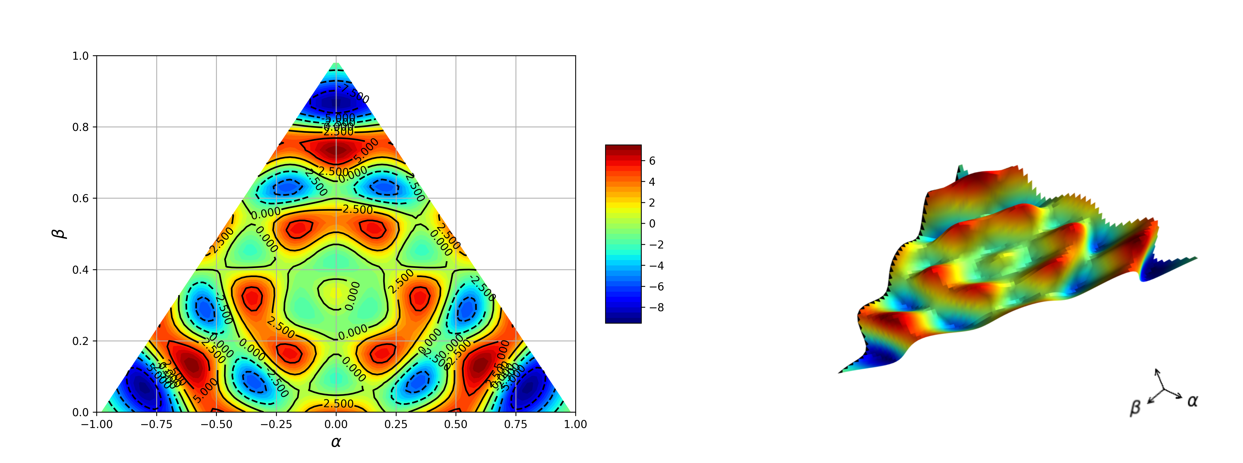
For one triangle of wavevectors in the bispectrum, it is often convenient to use a parameter to describe the overall scale, $k_{s}=k_{1}+k_{2}+k_{3}$, and two further parameters for the shape, $\alpha$ and $\beta$, defined as

$$\begin{split}k_{1}&=\frac{k_{s}}{4}(1+\alpha+\beta)\\ k_{2}&=\frac{k_{s}}{4}(1-\alpha+\beta)\\ k_{3}&=\frac{k_{s}}{2}(1-\beta),\end{split}$$ (6.2.3)

with the allowed values of $(\alpha,\beta)$ falling inside a triangle in the $\alpha$, $\beta$ plane with vertices $(-1,0)$, $(1,0)$ and $(0,1)$.

6.3 Model with a continuous curved trajectory

(a)

(b)

Figure 1: The time evolution of the polar coordinate fields $\theta$ and $R$ with metric (6.3.2) on the left, and the cartesian coordinates, $X$ and $Y$ on the right.

(a)

(b)

Figure 2: The time evolution of correlation functions. On the left the time evolution of the two-point function of the curvature perturbation, $\zeta$, and on the right the evolution of the three-point function for an equilateral configuration. Both were taken for modes exiting the horizon 21 e-folds before the end of inflation.

(a)

(b)

Figure 3: The reduced bispectrum $f_{nl}(k_{1},k_{2},k_{3})$ for equilateral configurations. On the left the evolution of $f_{nl}$ versus time for an equilateral configuration with modes leaving the horizon 21 e-folds prior to the end of inflation. On the right the bispectrum over a range of equilateral configurations as a function of exit time of the scale $k_{s}/3$.

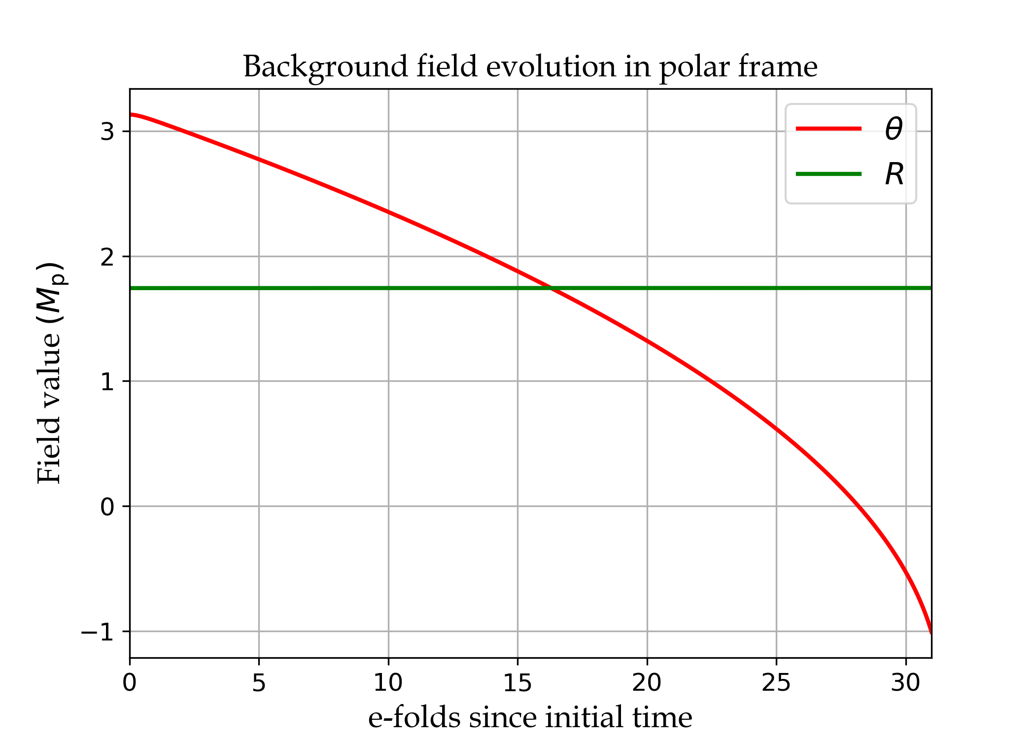
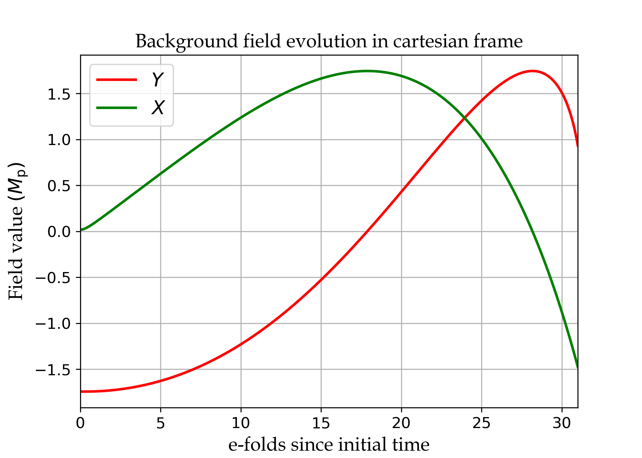
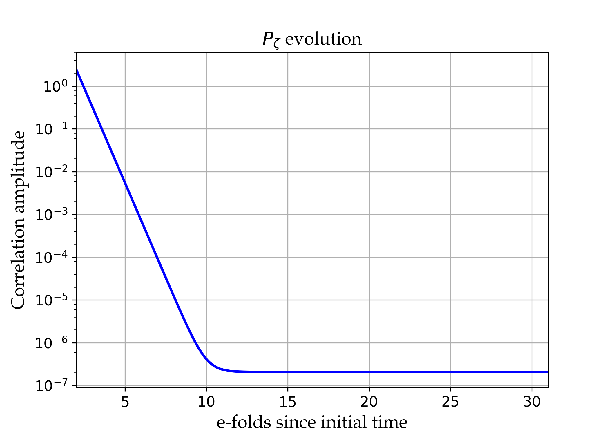
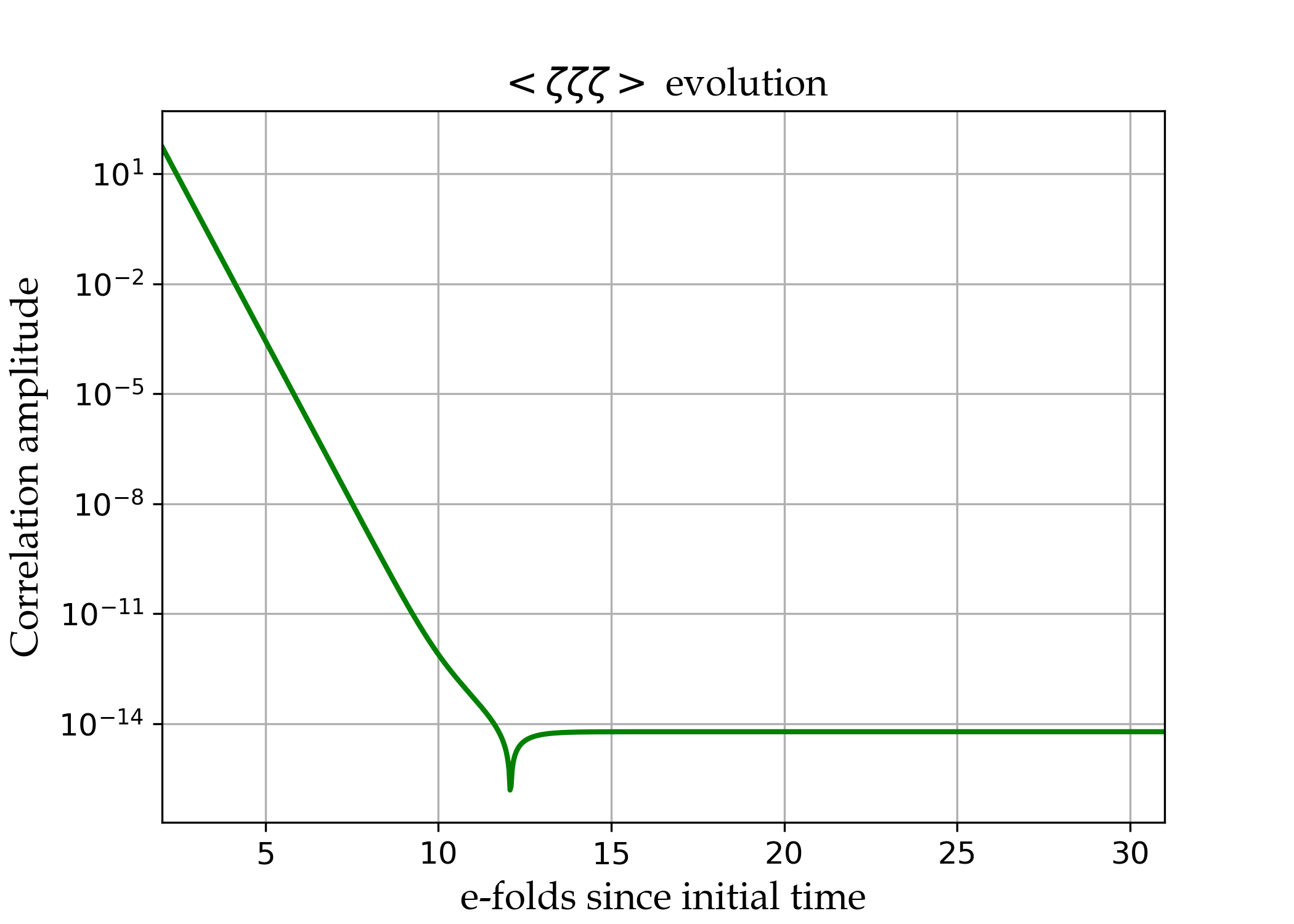
Ref. [1] attempted to construct a model in which the field-space trajectory was curved in such as way as to exhibit Gelaton [34] or QSFI [35] behaviour. For reasons presented there, this behaviour was difficult to achieve, but the model presented there is still a useful example, and in the present context provides a useful check of our code.

The model is defined by the action for two fields $R$ and $\theta$ as

$$S=-\frac{1}{2}\int d^{4}x\sqrt{-g}\left[(\partial R)^{2}+R^{2}(\partial\theta)^{2}+2V(R,\theta)\right]\,,$$ (6.3.1)

where the potential (defined below in Eq. (6.3.3)) represents a circular valley at a fixed value of $R$ – and hence is naturally written in terms of these ‘polar coordinate’ fields. However, as the codes developed for Ref. [1] only dealt with canonical kinetic terms, in that work it was necessary to perform a field redefinition to cartesian coordinates $X$ and $Y$. Here we evolve the statistics directly for the fields $R$ and $\theta$ and compare results, using this as a test case to benchmark our code against its canonical precursor.

The field-space metric of the model can be read off from Eq. (6.3.1), and is

$$G_{IJ}=\left(\begin{matrix}1&0\\ 0&R^{2}\end{matrix}\right)\,.$$ (6.3.2)

The potential is

$$V=V_{0}\left(1+\frac{29\pi}{120}\theta+\frac{1}{2}\frac{\eta_{\mathrm{R}}}{M_{\mathrm{p}}^{2}}(R-R_{0})^{2}+\frac{1}{3!}\frac{g_{\mathrm{R}}}{M_{\mathrm{p}}^{3}}(R-R_{0})^{3}+\frac{1}{4!}\frac{\lambda_{\mathrm{R}}}{M_{\mathrm{p}}^{3}}(R-R_{0})^{4}\right)\,,$$ (6.3.3)

and we choose parameters $V_{0}=10^{-10}M_{\mathrm{p}}^{4}$, $\eta_{\mathrm{R}}=1/\sqrt{3}$, $g_{\mathrm{R}}=M_{\mathrm{p}}^{2}V_{0}^{-1/2}$, $\omega=\pi/30$, $\lambda_{\mathrm{R}}=0.5M_{\mathrm{p}}^{3}\omega^{-1/2}V_{0}^{-3/4}$ and $R_{0}=\frac{30\sqrt{10^{-10}/3}}{\pi\sqrt{10^{-9}}}$. With these choices, the radial direction represents a heavy mode confining the inflationary trajectory to the valley, with angular direction light. We further choose initial conditions

$$R_{\mathrm{ini}}=\sqrt{R_{0}^{2}+(10^{-2}R_{0})^{2}}\quad{\rm and}\quad\theta_{\mathrm{ini}}=\arctan\left(\frac{10^{-2}R_{0}}{R_{0}}\right)\,.$$ (6.3.4)

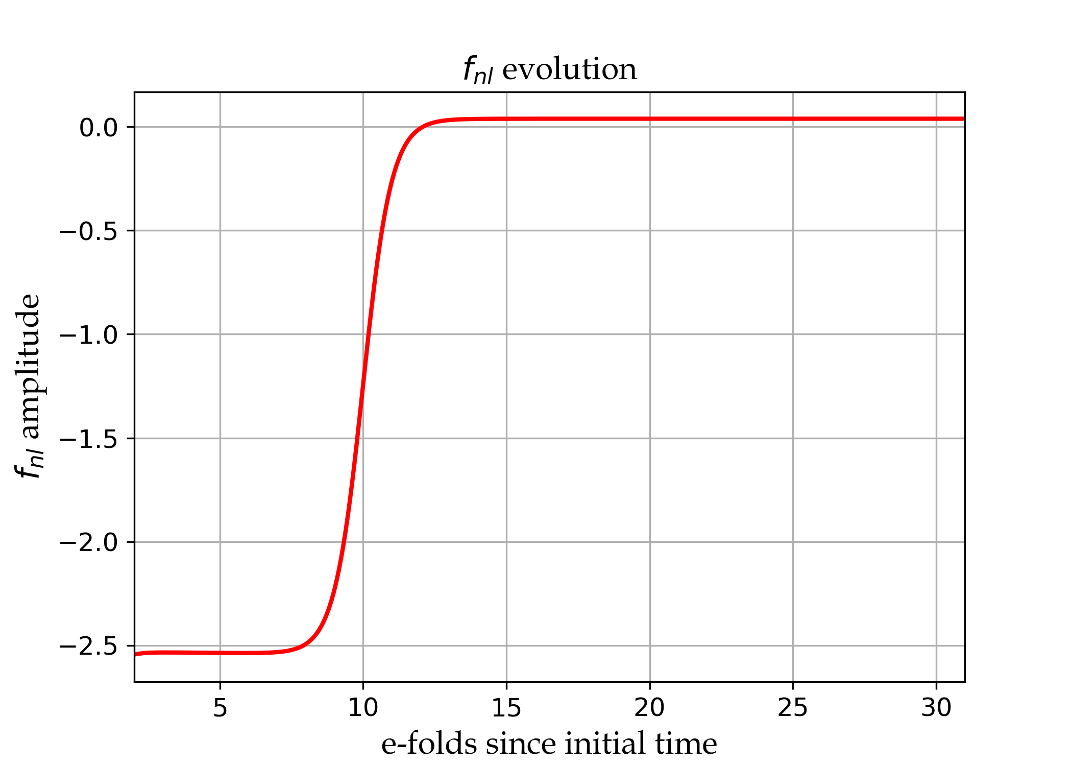
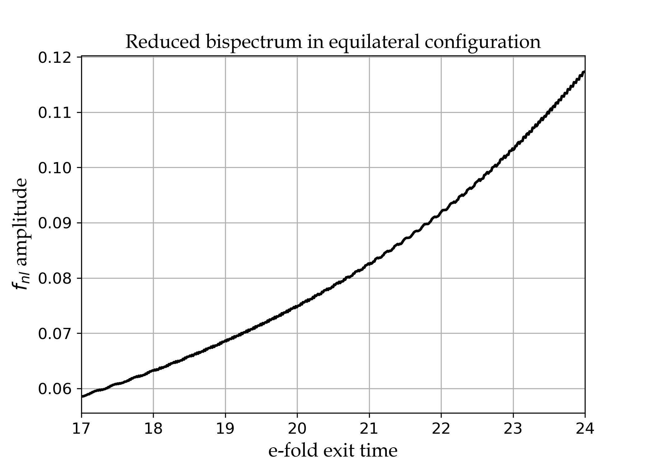
Generating results using our new code for the field evolution and correlations in the $\{R,\theta\}$ basis, and then subsequently using a coordinate transformation to translate the results to the $\{X,Y\}$ basis, we can compare our results to the output of the canonical code. We find excellent agreement. The evolution of correlation functions of the curvature perturbation, $\zeta$, are coordinate invariant, and also match that generated using the canonical code. In Fig. 1(a) the background field evolution in the non-canonical case is plotted. Under the coordinate transformation to the canonical fields $X$ and $Y$ we get the evolution in Fig. 1(b). In Fig. 2(a) & 2(b) one can clearly see that after horizon crossing the curvature perturbation freezes in, becoming constant on large scales as expected. The evolution of the reduced Bispectrum $f_{nl}$ for one equilateral triangle is shown in Fig. 3(a). The reduced bispectrum in the equilateral configuration as a function of horizon crossing time is given in Fig. 3(b), and can be compared with Fig. 11 of Ref. [1].

6.4 Quasi-two-field inflation

(a)

(b)

Figure 4: The time evolution of the fields $\phi_{1}$, $\phi_{2}$ and $\phi_{3}$ on the left, and the time evolution of the two-point function of $\zeta$ for a k-mode exiting the horizon 60 e-folds before the end of inflation on the right. The turn in field-space occurs 13 e-folds into inflation when the field $\phi_{2}$ experiences excitations from its coupling to the lighter field $\phi_{1}$ via the field-space metric. After roughly 30-e-folds the $\phi_{1}$ field reaches the minimum and the amplitude of the power spectrum increases at this time.

Figure 5: The power-spectrum of the curvature perturbation for a range of modes which exit the horizon over a window of 7 e-folds. The scale $k_{pivot}$ is taken to be when the mode leaves the horizon at 58 e-folds prior to the end of inflation. Both the scales and amplitudes are normalised to the spectrum at the pivot scale.

(a)

(b)

Figure 6: The evolution of the three-point function for one equilateral configuration, and the reduced bispectrum, $f_{nl}$, for equilateral configurations over a range $k_{s}$. The reduced bispectrum is plotted for modes leaving the horizon between 59 and 51 e-folds before the end of inflation. The highly oscillatory behaviour is a result of the excitations to the heavy field around horizon crossing.

Figure 7: Amplitude over shape configurations of the reduced bispectrum ${f_{nl}}(\alpha,\beta)$ at a fixed $k_{t}$ 53 e-folds before the end of inflation, corresponding to $\log(k/k_{pivot})=4.79$.

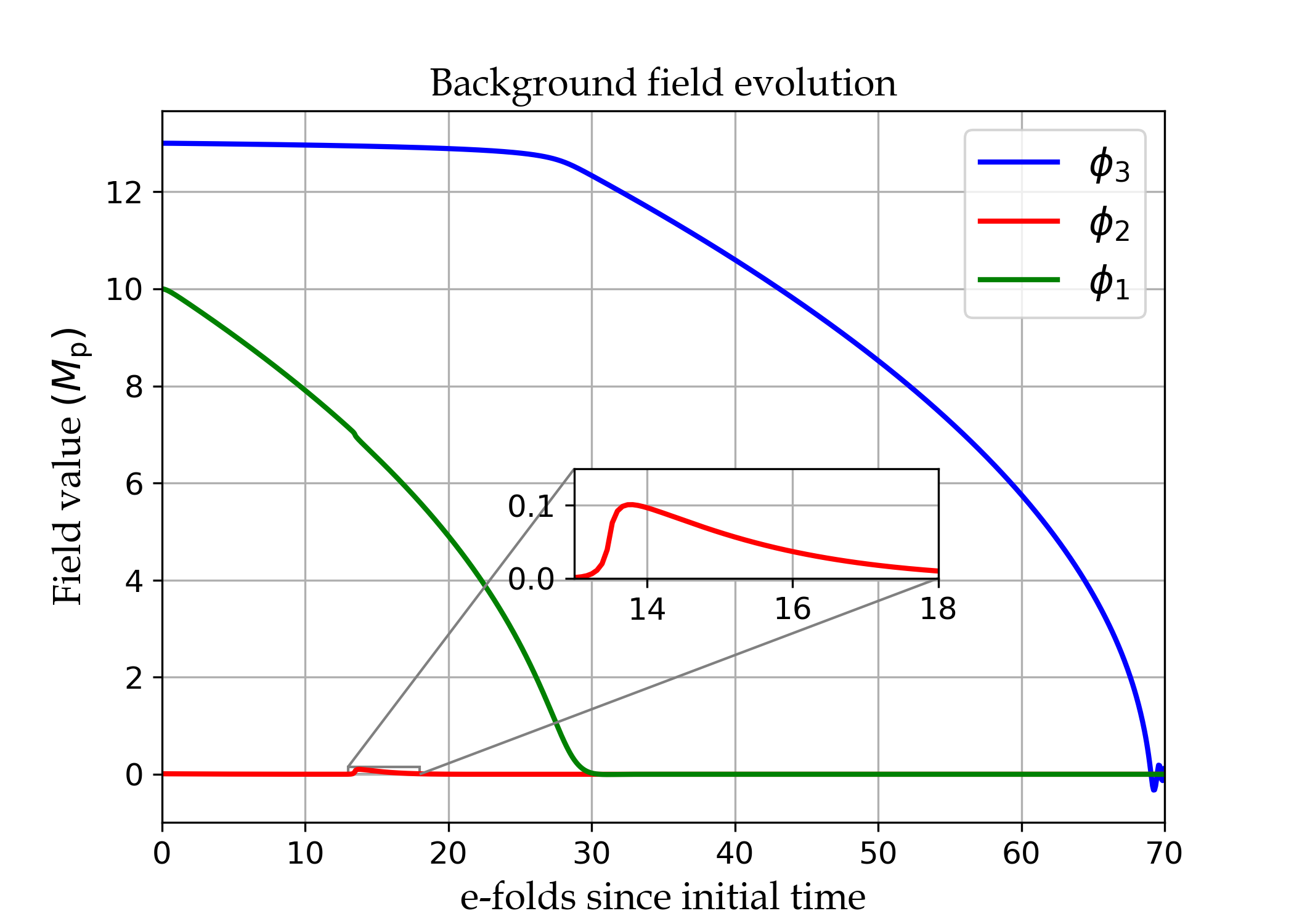
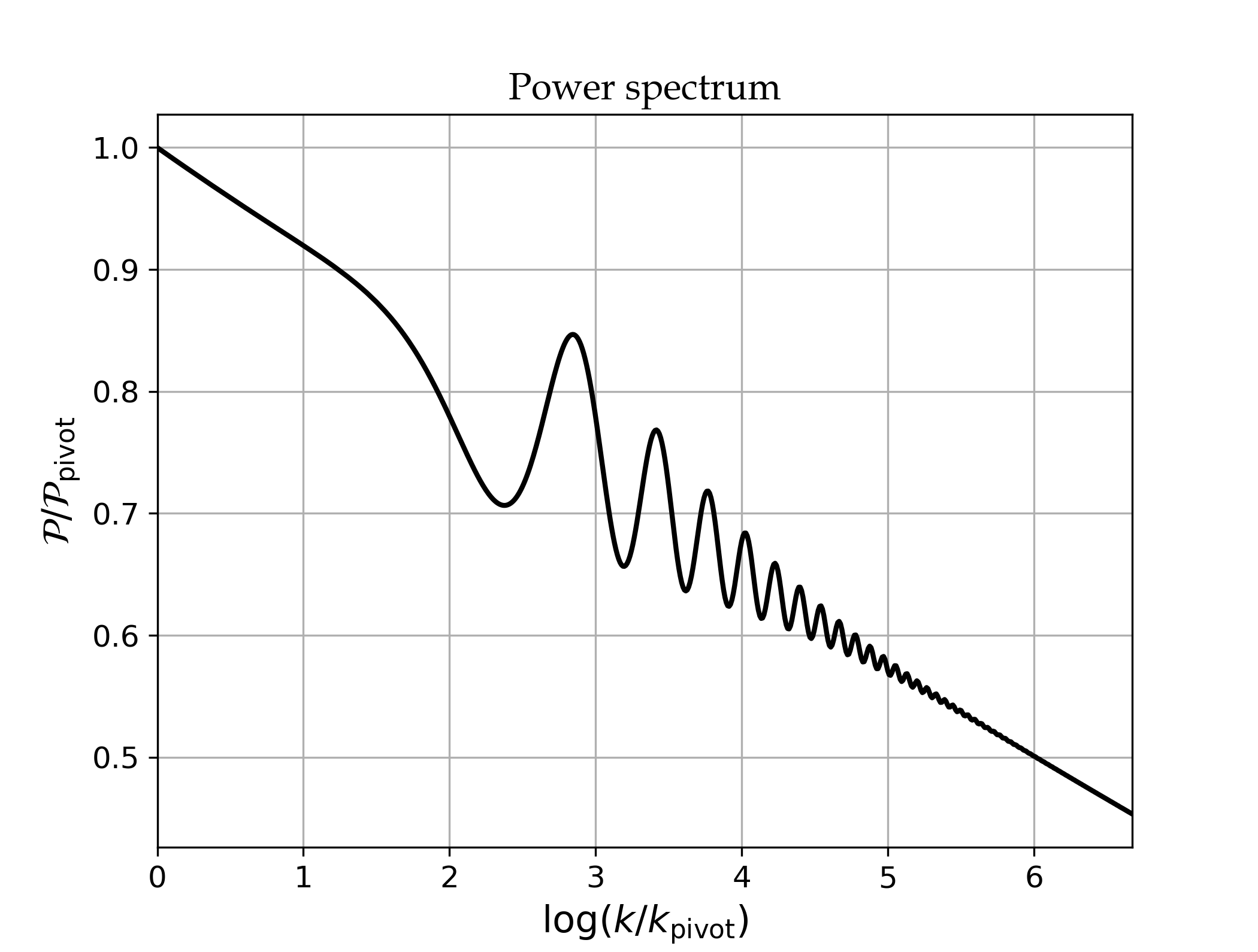
Next we consider the quasi-two field model introduced in Ref. [10] where the power spectrum was calculated. In this model there are two light scalar fields which drive inflation and one heavy field which interacts with the light ones through a coupling in the kinetic terms. This leads to a fast turn in the plane of the lighter two fields resulting in the well known feature of oscillations in the power spectrum and bispectrum (see for example [36, 37, 38, 39, 40, 41, 42, 43]). In this paper we reproduce the power spectrum presented in Ref. [10] as a test of our code and then calculate the bispectrum for the first time. The three fields are labelled $\phi_{1}$, $\phi_{2}$ and $\phi_{3}$, and model has a metric which takes the form

$$G_{IJ}=\left(\begin{matrix}1&\Gamma(\phi_{1})&0\\ \Gamma(\phi_{1})&1&0\\ 0&0&1\end{matrix}\right)\,.$$ (6.4.1)

The function $\Gamma(\phi_{1})$ has the following $\phi_{1}$ dependence [44],

$$\Gamma(\phi_{1})=\frac{\Gamma_{0}}{\cosh^{2}\left(2\left(\frac{\phi_{1}-\phi_{1(0)}}{\Delta\phi_{1}}\right)\right)}\,,$$ (6.4.2)

with $\Gamma_{0}=0.9$ the maximum value attained by $\Gamma(\phi_{1})$. $\phi_{1(0)}=7M_{\mathrm{p}}$ is the value of $\phi_{1}$ at the apex of the turn in field-space and $\Delta\phi_{1}=0.12$ is the range of $\phi_{1}$ over which the turn occurs The potential is defined as

$$V=\frac{1}{2}g_{1}m^{2}\phi_{1}+\frac{1}{2}g_{2}m^{2}\phi_{2}+\frac{1}{2}g_{3}m^{2}\phi_{3}\,,$$ (6.4.3)

with parameters $g_{1}=30$, $g_{2}=300$, $g_{3}=30/81$ and $m=10^{-6}$. The initial conditions of the fields are

$$\phi_{1}=10.0M_{\mathrm{p}}\quad\phi_{2}=0.01M_{\mathrm{p}}\quad\phi_{3}=13.0M_{\mathrm{p}}\,.$$ (6.4.4)

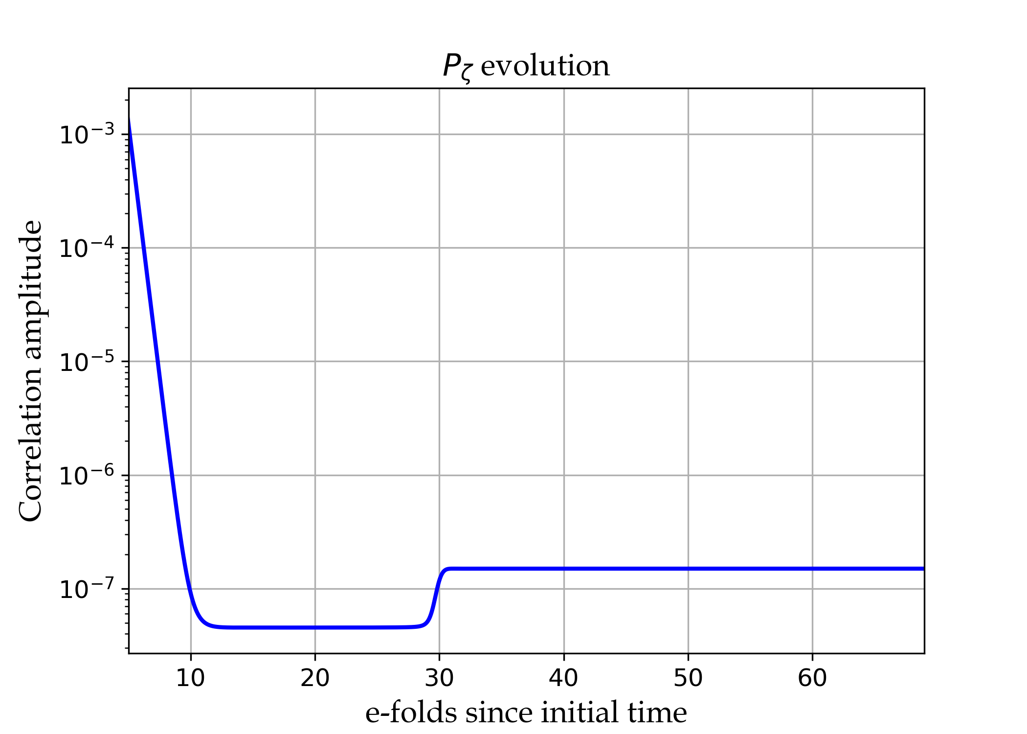
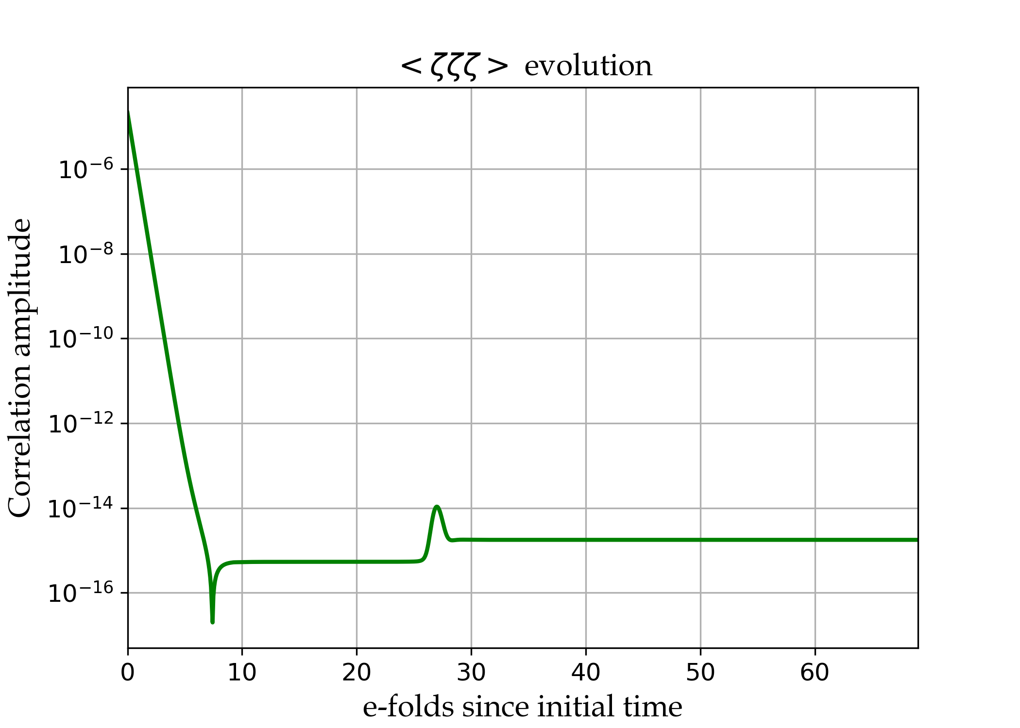
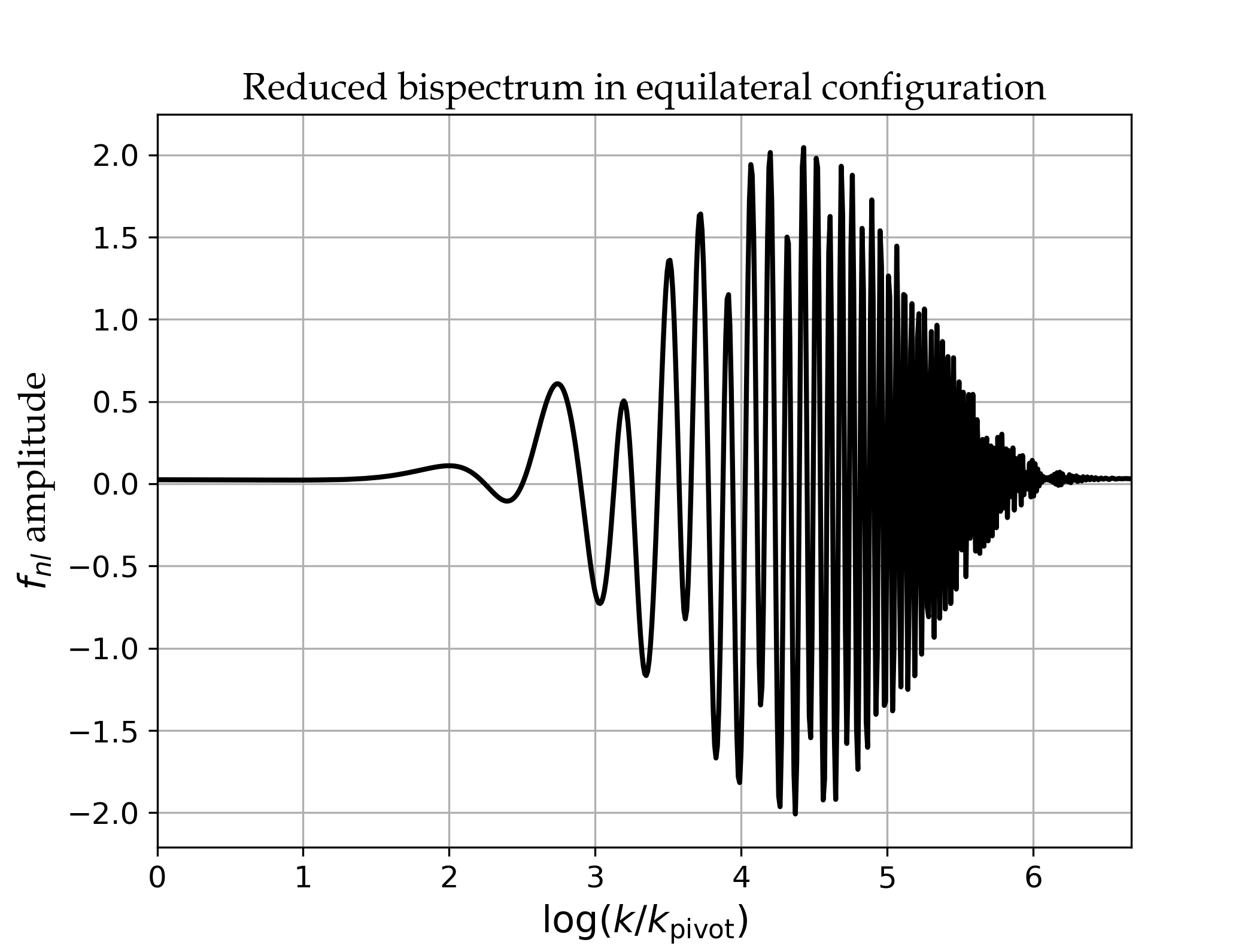
In Fig. 4(a) the background field evolution is plotted. At 13 e-folds into the evolution the turn in the inflationary trajectory occurs, as can be seen by the increase in the amplitude of the heaviest field. In Figs. 4(b) & 6(a) the evolution of both the two and three-point correlation functions of curvature perturbations are plotted. The power spectrum obtained in Fig. 5 matches that seen in Ref. [10] illustrating that the code is in good agreement with this earlier implementation. We produce the reduced bispectrum over equilateral configurations in Fig. 6(b), the structure of which is defined by a pulse of large and rapidly oscillating values of the three-point function. Finally, for a fixed scale $k_{t}$ we plot the reduced bispectrum in Fig. 7 as a function of the $\alpha$ and $\beta$ parameters discussed in §6.2 for a fixed $k_{t}$.

6.5 Inflation on a 2-sphere metric

(a)

(b)

Figure 8: The evolution of the fields $\theta$ and $\psi$ on the left and the evolution two-point function of the curvature perturbation on the right for a mode leaving the horizon 50 e-folds prior to the end of inflation. From 30 e-folds into inflation until the end there is no further evolution of the two-point function.

(a)

(b)

Figure 9: Evolution of the reduced bispectrum in an equilateral configuration on the left and the reduced bispectrum for an equilateral configuration versus the radius of the metric sphere on the right. From 30 e-folds into inflation until the end there is no further evolution of $f_{nl}$. The evolution of $f_{nl}$ was taken for a mode leaving the horizon at 26 e-folds from the beginning of inflation. The bispectrum on the right is taken for a range of modes in the window between 25 and 30 e-folds and for a radius between 9 and 11.5. It illustrates a large amplitude correlation over scales for a small radius (or rather large field-space curvature).

In the models considered above the field-space metrics were non-trival, but flat. As a further test of our code, therefore, we now introduce a model with a constant non-zero Ricci curvature.

We construct a toy model containing two fields $\theta$ and $\psi$, where the action is defined as

$$S=-\frac{1}{2}\int d^{4}x\sqrt{-g}\left[r_{0}^{2}(\partial\theta)^{2}+r_{0}^{2}\sin^{2}\theta(\partial\psi)^{2}+2V(\theta,\psi)\right]\,,$$ (6.5.1)

where $r_{0}$ is the radius of the surface of the sphere which the field trajectory is confined to. The curvature of the field-space, defined by the Ricci Scalar, is related to the radius, $R=\frac{2}{r^{2}_{0}}$. The field-space metric which describes the line element along the surface of a sphere is therefore

$$G_{IJ}=\left(\begin{matrix}r_{0}^{2}&0\\ 0&r_{0}^{2}\sin^{2}\theta\end{matrix}\right).$$ (6.5.2)

For the potential we use the same potential given for the axion-quartic model studied in Ref. [1]. The potential is of the form,

$$V=\frac{1}{4}g_{\theta}\theta^{4}+\Lambda^{2}\left(1-\cos\left(\frac{2\pi\psi}{f}\right)\right)\,,$$ (6.5.3)

where the field $\psi$ is our “2-sphere-axion” and our parameters are $g_{\theta}=10^{-10}$, $\Lambda^{4}=(25/2\pi)^{2}gM_{\mathrm{p}}^{4}$, $\omega=30/\pi$ and $f=M_{\mathrm{p}}$. The initial conditions of the fields are set to

$$\theta_{\rm ini}=2.0M_{\mathrm{p}}\quad and\quad\phi_{\rm ini}=f/2-10^{-3}M_{\mathrm{p}},$$ (6.5.4)

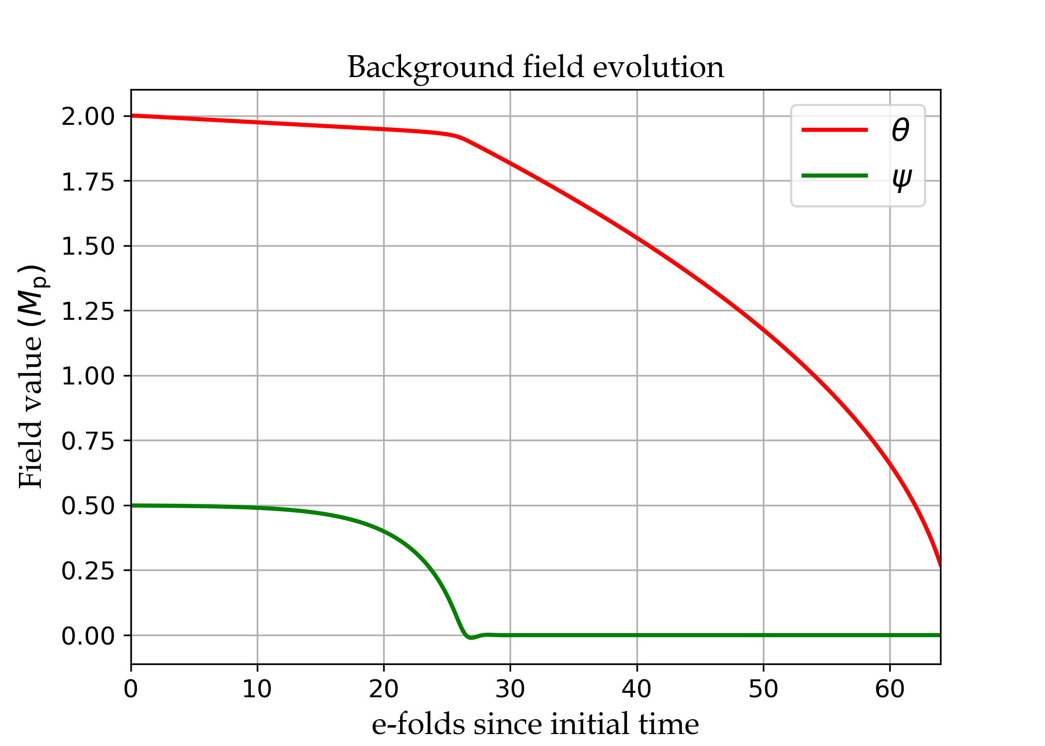
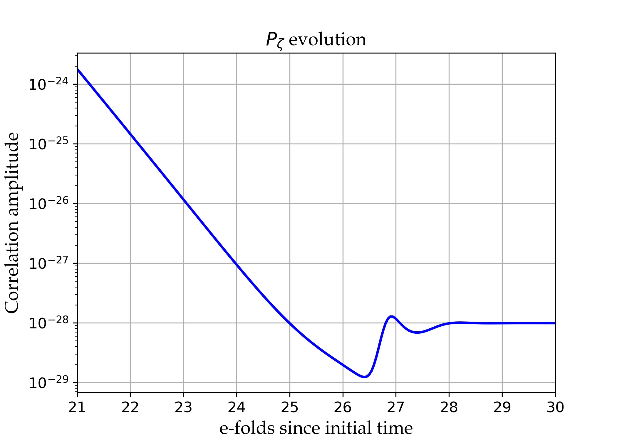
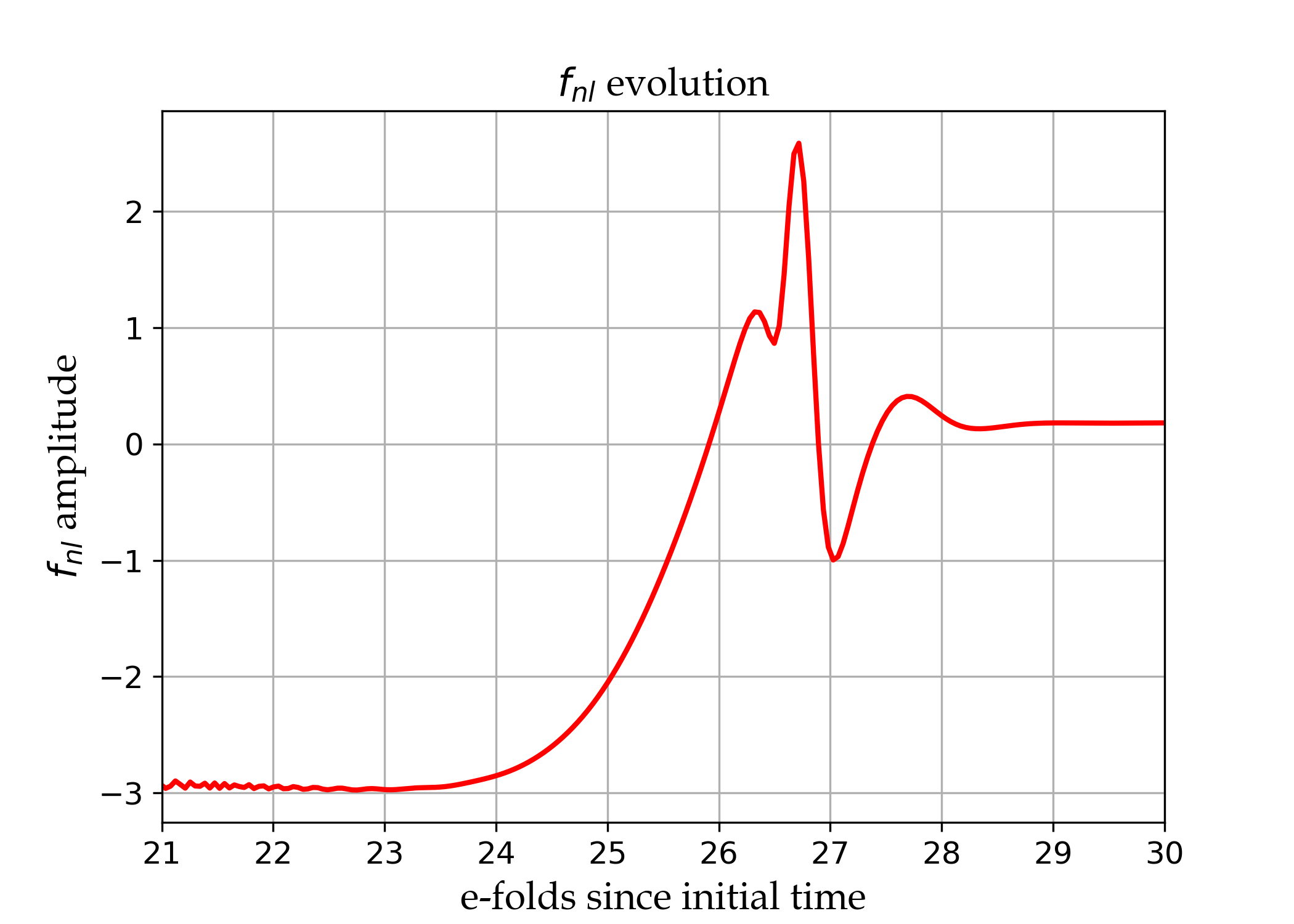
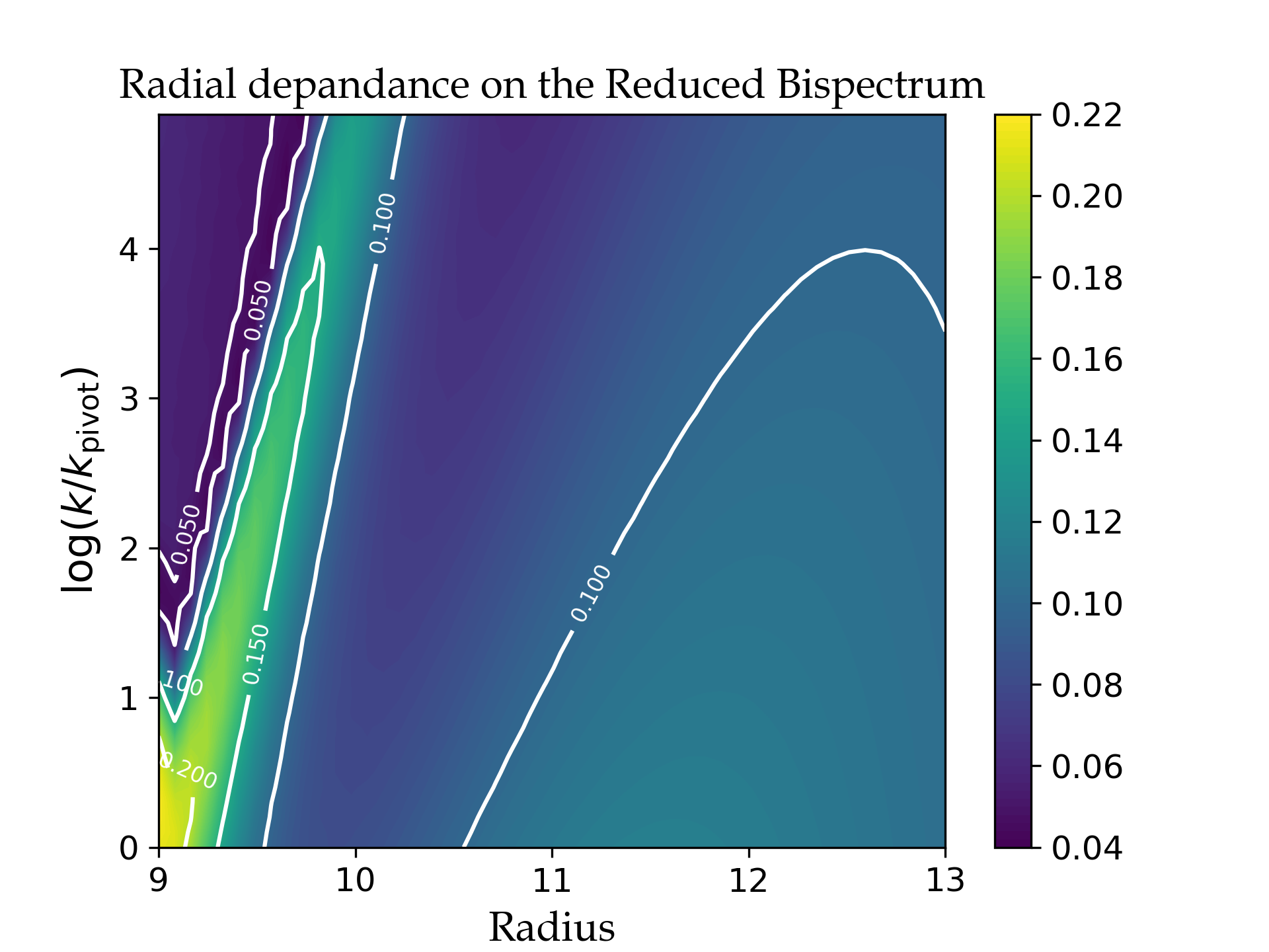
which is sufficient for inflation for 64 e-folds. The background evolution of the fields are plotted in Fig. 8(a), with the corresponding evolution of correlations of the curvature perturbations for two-point (Fig. 8(b)) and three-point (Fig. 9(a)) functions. We study the effects of curvature on quantities like the bispectrum by varying the radius $r_{0}$. Figure  9(b) is a contour graph of the bispectrum as a function of $r_{0}$. We see that for a radius $r_{0}>11.0$ the bispectrum is small, but for $r_{0}<11.0$ the bispectrum begins to increase. This indicates a correlation between large curvature and a value of large $f_{nl}$ in this model.

6.6 Inflation on a conifold metric

Figure 10: The evolution of the 6 moduli fields during inflation. Rich dynamics exist owing to the couplings in the conifold metric. Inflation ends when the branes collide at a value of $r=0$.

(a)

(b)

Figure 11: On the left, the power spectrum of curvature perturbation and on the right the bispectrum of curvature perturbations over an equilateral configuration for modes exiting the horizon after a large range of times between 12 and 64 e-folds.

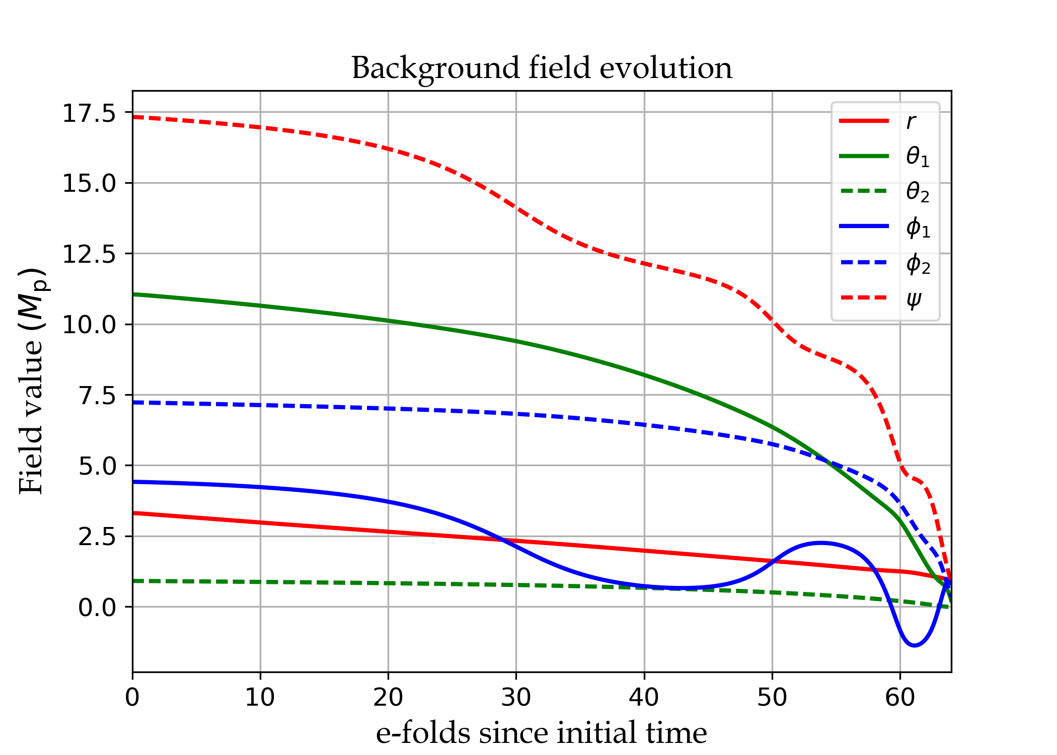
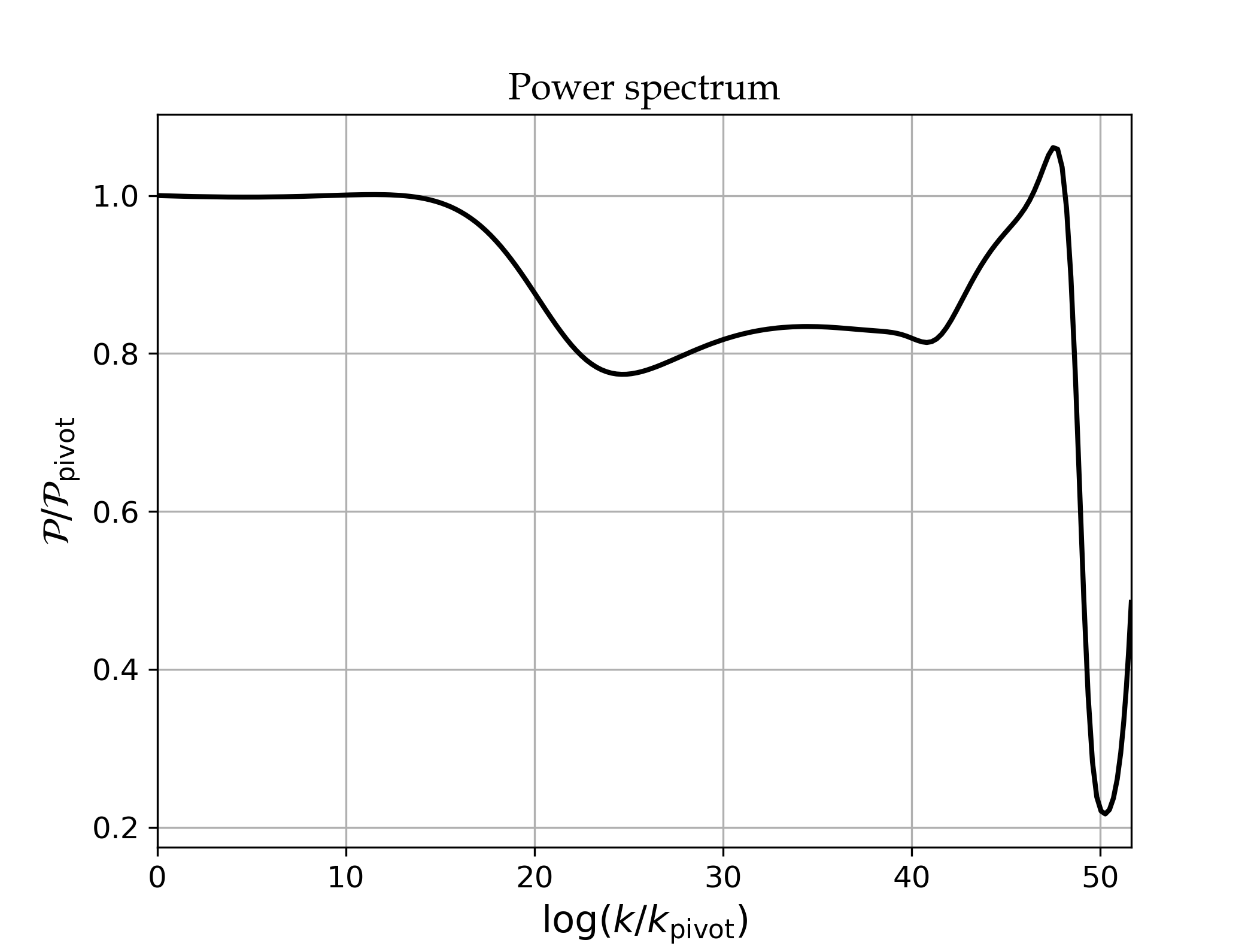
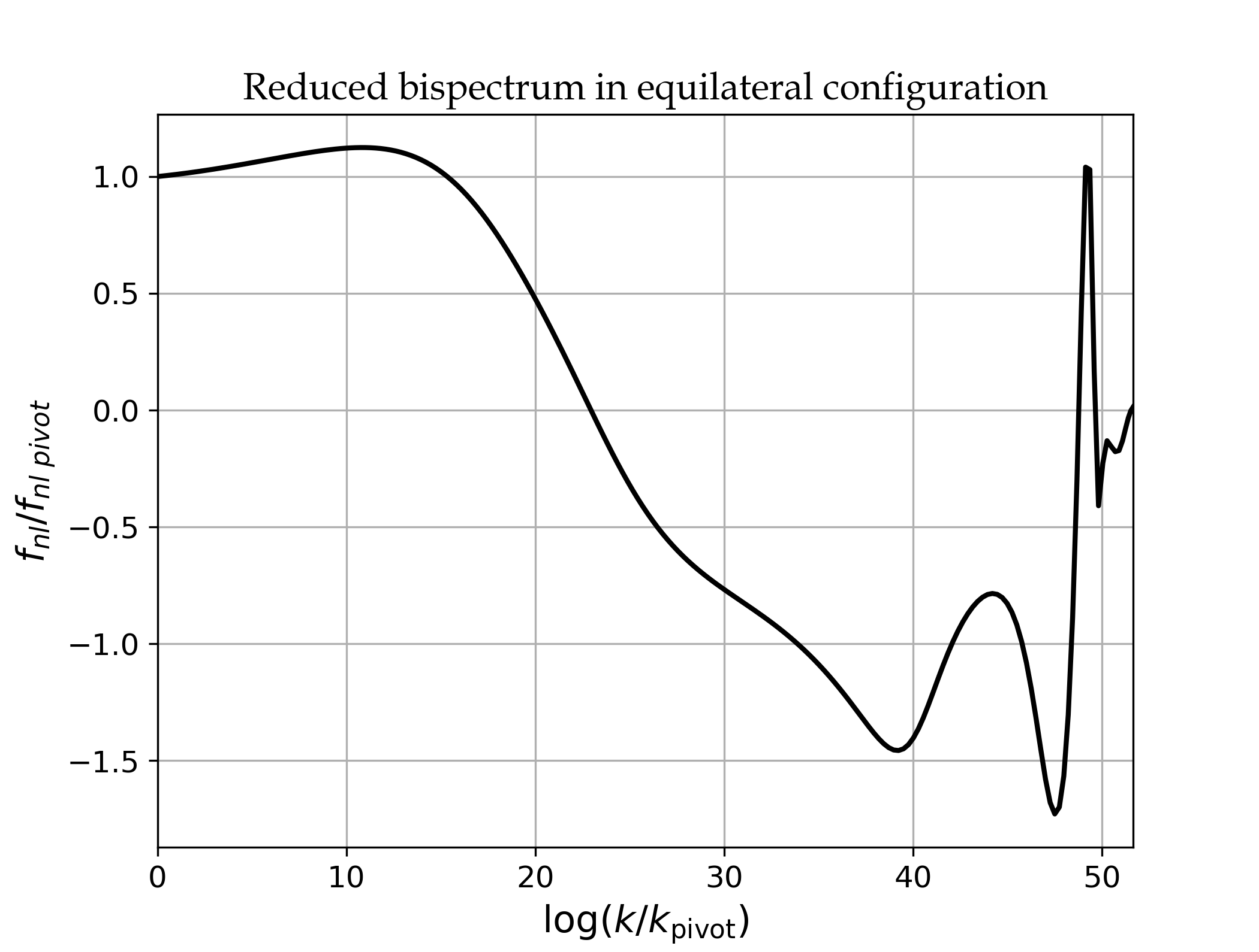
Finally we consider a more realistic case inspired by models of D-brane inflation. Such models have recently been the subject of considerable interest, with a number of groups statistically probing their realisations [45, 46, 47]. In one such scenario two D3-branes are attracted by a Coulomb force. Compactification induces a warping of the 6-D manifold where the D3-brane sits, resulting in a non-trivial field-space metric in the Lagrangian of the system. Both the geometry of the metric and structure of the potential affect the inflationary dynamics. Initial work [45] looked at the background dynamics of this system, while more recent studies looked into the distribution of 2-point statistics [46, 47]. Here we illustrate how our new code could be used to obtain information about the bispectrum, though we defer realistic studies to future work.

We consider the Lagrangian of D3-brane inflation as

$$S=-\frac{1}{2}\int d^{4}x\sqrt{-g}\left(G_{IJ}d\phi^{I}d\phi^{J}+2V(\phi_{1},\dots\phi_{6})\right),$$ (6.6.1)

where $a$ is the scale factor. The scalar fields represent the 6 brane coordinates, one radial $r$ and five angular dimensions $\theta_{1},\theta_{2},\phi_{1},\phi_{2}$ and $\psi$. The field-space metric $G_{IJ}$ corresponds to the Klebanov-Witten conifold geometry [48]. The metric is of the form,

$$G_{IJ}d\phi^{I}d\phi^{J}=dr^{2}+r^{2}d\Omega^{2}\,,$$ (6.6.2)

with the metric of the cone $d\Omega$ [49] is given by

$$d\Omega^{2}=\frac{1}{6}\sum^{2}_{i=1}\left(d\theta_{i}^{2}+\sin^{2}\theta_{i}d\phi_{i}^{2}\right)+\frac{1}{9}\left(d\psi+\sum^{2}_{i=1}\cos\theta_{i}d\phi_{i}\right)^{2}\,,$$ (6.6.3)

which is a non-compact geometry built over the five-dimensional $(SU(2)\times SU(2))/U(1)$ coset space $T^{1,1}$. As a toy example we do not generate a realistic potential (motivated by any attractive forces between branes or contribution from either the homogeneous or the inhomogeneous bulk), instead, for simplicity, we take a quadratic potential for the 6 fields

$$V(\phi)=\sum^{6}_{i=1}m_{i}^{2}\phi_{i}^{2}\,,$$ (6.6.4)

where $m_{i}$ are the randomised masses of the fields. A randomised set of masses and initial conditions are selected with the criteria that 64 e-folds of inflation occur. With these parameters the evolution of the dynamics and statistics can be run and the background trajectory for each of the six fields is plotted in Fig. 10. The power spectrum is plotted in Fig. 11(a) and the bispectrum in the equilateral configuration is plotted in Fig. 11(b). It would be interesting to run a more realistic analysis including the full potential of the system but this is beyond the scope of our work. We have, however, demonstrated that this is possible using the transport method and its implementation in code via PyTransport.

6.7 Performance

Figure 12: Top panel: scaling of integration time with increasing number of massless (or subhorizon) e-folds (using relative and absolute tolerances of $10^{-8}$) for an equilateral triangle of the bispectrum and a squeezed triangle ($\alpha=0$, $\beta=0.99$). Timings were performed using the canonical code and the new non-canonical code setting a Euclidean metric explicitly. Bottom panel: scaling of integration time with integration tolerance with 5 e-folds of massless evolution. The double quadratic model used to analysis performance in Ref. [1] is timed using the canonical PyTransport package and compared to the same model using PyTransport 2.0. The computer used for timings contained an 3.1 GHz Intel i7-4810MQ processor.

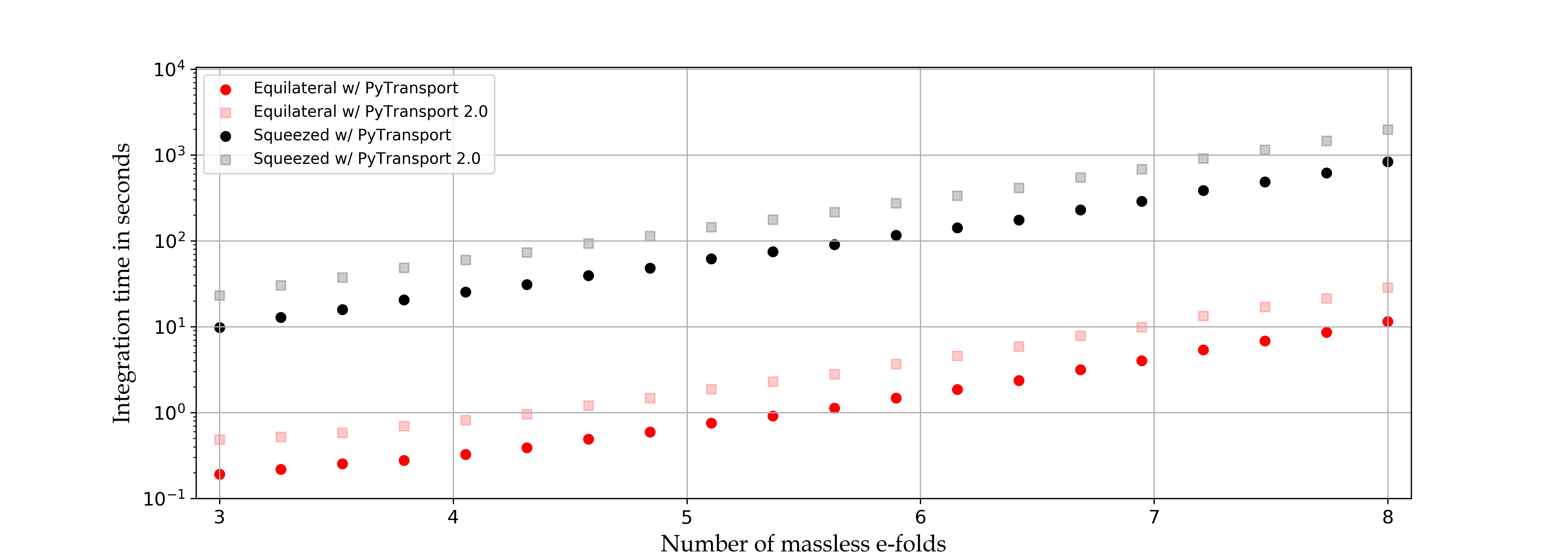
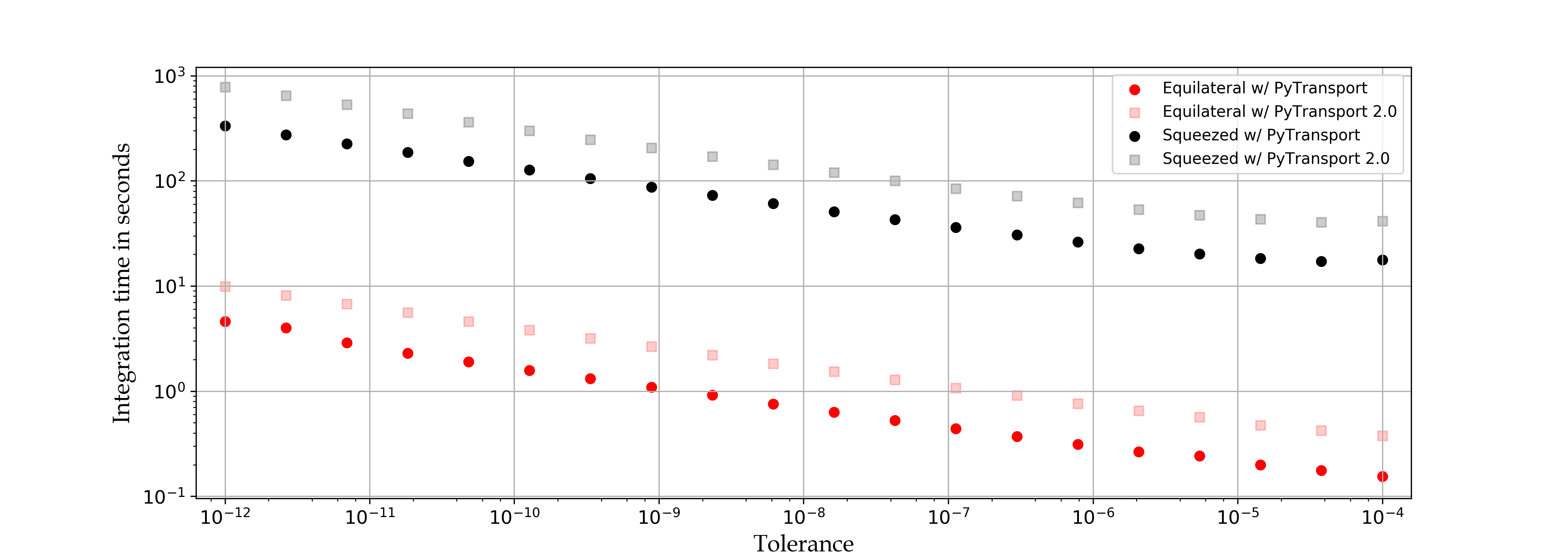
In PyTransport 2.0, one can opt to specify explicitly a field space metric. If this option is not selected the code defaults to assuming that the metric is Euclidean and the code reverts back to the previous canonical code. The simplicity of a Euclidean metric means that a number of internal loops do not need to be performed, and hence the canonical code is expected to be faster than when a metric is specified explicitly (even if the metric is the Euclidean one). To demonstrate this effect and also to benchmark the speed of the new code in Fig. 12 we show how the speed of the new code compares with that of the canonical one. We also show how the speed of the code is sensitive to the number of e-folds before horizon crossing (of the shortest scale in the triangle being evaluated) at which initial conditions are fixed, and to different tolerances which fix the accuracy of the code. For this purpose we use the double quadratic potential used to calculate performance data in Ref. [1]. As can be seen, the new code is roughly a factor of 2 slower for this two field model. We find that introducing a simple field space metric, such as the 2-sphere metric used in § 6.5, leads to very similar timing data to the Euclidean metric (though more complicated metrics will inevitably slow down the code as the terms in the metric need to be evaluated at each time step). A more significant effect comes from increasing the number of fields. The size of the arrays which store information about the Riemann tensor and its derivative scale as ${\cal N}^{4}$ and ${\cal N}^{5}$ respectively (for the canonical code the largest arrays scale as ${\cal N}^{3}$), and therefore memory issues and overheads resulting form accessing and looping over these arrays grow rapidly as field number increases.

7 Conclusion

We have extended the method of calculating the power spectrum and bispectrum developed in Ref. [1] for canonical multi-field inflation to include models which contain a non-trivial field-space metric. First in §2 the equations of motion and the conservation equations for perturbations were derived for our non-canonical multi-field system. We reviewed how the system of equations can be written as an autonomous system for a set of covariant “field” perturbations. Next we reviewed how the transport method is applied in combination with these equations to give equations for the evolution of the correlations of the covariant perturbations during inflation. To use this system in practice we needed to calculate both initial conditions for our new system of equations, and the relation between covariant field-space perturbations and the curvature perturbation $\zeta$. A neat result we found is that our expressions for these quantities take the form of the covariant versions of the expressions presented in Ref. [1], with no additional Riemann terms appearing (except through the new terms that appear in the $a$, $b$ and $c$ tensors which define the equations of motion).

We have demonstrated explicitly that our method is successful in evaluating the observable statistics of inflationary models with many fields and a curved field-space metric. The code we have developed to do this is the second iteration of the PyTransport package, PyTransport 2.0, and agrees with its predecessor in the case of models which can be written in Euclidean and non-Euclidean coordinates (as discussed in § 6.3). Moreover, we have shown that for simple 2-field models that the speed of the new code compares with well with that of the canonical model. It should be noted, however, that the the code has not been tested for models exceeding more than six fields, and that we expect time taken to scale poorly with number of fields. Our hope is that this new code will be useful to the inflationary cosmology community.

Appendix A Initial Conditions

Here we provide a few more detail of how the initial conditions for the transport system are calculated. We recall that $\star$ denotes a time long before horizon crossing at which $-\tau\gg 1$, where $\tau$ denotes conformal time, and that for a de-Sitter expansion $\tau=-1/(aH)$.

A.1 Two point function

First we consider initial conditions for the two point function for the various combinations of covariant field perturbation and momenta correlations. The calculation is similar to that presented in Ref. [10], though in that work the time variable used for the transport system was e-folds $N$, while in this paper we use cosmic time, $t$.

• Field-Field correlation

Beginning with the expression for the two point function of $Q^{I}$ (4.0.1) we consider the $-\tau\gg 1$ limit for the field-field correlations. We find

$$\begin{split}\langle Q^{I}(k_{1},\tau)Q^{J}(k_{2},\tau)\rangle&=(2\pi)^{3}\delta(k_{1}+k_{2})\frac{G^{IJ}}{2k^{3}}H^{2}(\tau)(1-ik\tau)(1+ik\tau)\\ &\approx(2\pi)^{3}\delta(k_{1}+k_{2})\frac{G^{IJ}}{2k^{3}}H^{2}(\tau)|k\tau|^{2}\\ &\approx(2\pi)^{3}\delta(k_{1}+k_{2})\frac{G^{IJ}}{2a^{2}k}\,.\end{split}$$ (A.1.1)

The initial condition for $\Sigma^{IJ}_{*}$ is then

$$\Sigma^{IJ}_{*Re}=\left.\frac{G^{IJ}}{2a^{2}k}\right|_{*}\,,\quad\Sigma^{IJ}_{*Im}=0\,.$$ (A.1.2)

• Field-Momentum correlation

Next recalling that at linear order $P^{I}=D_{t}Q^{I}$ and that the covariant derivative of the parallel propagator is zero, we consider the leading term in the expression for the field-momentum correlation of unequal time correlations, and subsequently take equal time limit for the case $-\tau\gg 1$. Recalling that $d\tau=dt/a(t)$ we find

$$\begin{split}\langle Q^{I}(k_{1},\tau_{1})P^{J}(k_{2},\tau_{2})\rangle&=(2\pi)^{3}\delta(k_{1}+k_{2})\frac{\Pi^{IJ}}{2k^{3}}H(\tau_{1})H(\tau_{2})(1+ik\tau_{1})\left(\frac{k^{2}\tau_{2}}{a}\right)e^{ik(\tau_{2}-\tau_{1})}\\ &=(2\pi)^{3}\delta(k_{1}+k_{2})\frac{G^{IJ}}{2k^{3}}H^{2}(\tau)\left(\frac{k^{2}\tau}{a}\right)(1-ik\tau)\\ &=(2\pi)^{3}\delta(k_{1}+k_{2})\left(-\frac{G^{IJ}H}{2ka^{2}}+i\frac{G^{IJ}}{2a^{3}}\right).\end{split}$$ (A.1.3)

The real and imaginary parts of the initial conditions for this case are then

$$\Sigma^{IJ}_{*Re}=\left.-\frac{G^{IJ}H}{2ka^{2}}\right|_{*}\,,\quad\Sigma^{IJ}_{*Im}=\left.\frac{G^{IJ}}{2a^{3}}\right|_{*}\,.$$ (A.1.4)

• Momentum-Momentum correlation

We follow a similar procedure to consider the momentum-momentum correlation

$$\begin{split}\langle P^{I}(k_{1},\tau_{1})P^{J}(k_{2},\tau_{2})\rangle&=(2\pi)^{3}\delta(k_{1}+k_{2})\frac{\Pi^{IJ}}{2k^{3}}H(\tau_{1})H(\tau_{2})\left(\frac{k^{2}\tau_{1}}{a}\right)\left(\frac{k^{2}\tau_{2}}{a}\right)e^{ik(\tau_{2}-\tau_{1})}\\ &=(2\pi)^{3}\delta(k_{1}+k_{2})\frac{G^{IJ}}{2k^{3}}H^{2}(\tau)\left(\frac{k^{4}\tau^{2}}{a^{2}}\right)\\ &=(2\pi)^{3}\delta(k_{1}+k_{2})\frac{G^{IJ}k}{2a^{4}}.\end{split}$$ (A.1.5)

The initial condition for $\Sigma^{IJ}$ in this case is

$$\Sigma_{*Re}^{IJ}=\left.\frac{G^{IJ}k}{2a^{4}}\right|_{*}\,,\quad\Sigma_{*Im}^{IJ}=0\,.$$ (A.1.6)

A.2 Three point function

For the three-point function as discussed in the main text, an integral must be evaluated to calculate the initial condition. By substituting Eq. (4.0.11) into Eq. (4.0.10) we obtain the initial condition $B_{*}^{abc}$. To illustrate how this is evaluated in practice, let us consider this explicitly for the case of a field-field-field correlation.

• a,b,c $\rightarrow$ Field-Field-Field

Substituting in the expression for the two-point function we obtain

$$\begin{split}B_{*}^{abc}=&-\frac{iH^{6}}{8\Pi_{i}k_{i}^{3}}(1+ik_{1}\tau)(1+ik_{2}\tau)(1+ik_{3}\tau)e^{-ik_{s}\tau}\times\\ &\int^{\tau_{init}}_{-\infty}\frac{d\eta}{H^{2}\eta^{2}}\left[\frac{\dot{\phi}^{I}G^{JK}}{4H}({\bf{k_{2}}}\cdot{\bf{k_{3}}})(1-ik_{1}\eta)(1-ik_{2}\eta)(1-ik_{3}\eta)e^{ik_{s}\eta}\right.\\ &+\frac{a^{IJK}_{s}}{2H^{2}\eta^{2}}(1-ik_{1}\eta)(1-ik_{2}\eta)(1-ik_{3}\eta)e^{ik_{s}\eta}\\ &+\frac{b^{IJK}}{2H^{2}\eta^{2}}(1-ik_{1}\eta)(1-ik_{2}\eta)k_{3}^{2}\eta e^{ik_{s}\eta}\\ &\left.+\frac{c^{IJK}}{2}k^{2}_{1}k^{2}_{2}\eta^{2}(1-ik_{3}\eta)e^{ik_{s}\eta}+perms\right]+c.c.\,,\end{split}$$ (A.2.1)

where we assume that $H$ and $\Pi^{IJ}$ are sufficiently slowly varying to be taken as constants and that we can take $\Pi^{IJ}\to G^{IJ}$.

In order to perform the integration we need to know the time dependence of the tensors. As discussed in §4 the $a_{IJK}$ tensor contains fast and slow varying parts. The part containing terms quadratic in $\eta$ vary quickly and so are included in the integral separately (the first term in Eq. (A.2.1)), the remaining parts we label $a_{s}^{IJK}$ and we assume can be considered constant in time. The next step is to perform the integration recalling that the result is dominated by the upper limit (because the integral is highly oscillatory into the past). Keeping the leading and sub-leading terms in $\tau$, and writing in terms of $a$ and $H$, the final result is

$$\begin{split}B^{abc}_{*}=&\frac{1}{4a^{4}}\frac{1}{{{k_{1}}}\cdot{{k_{2}}}\cdot{{k_{3}}}\cdot k_{s}}\left(-c^{IJK}(k_{1},k_{2},k_{3})\cdot({{k_{1}}}\cdot{{k_{2}}})-c^{IKJ}(k_{1},k_{3},k_{2})\cdot({{k_{1}}}\cdot{{k_{3}}})\right.\\ &-c^{JKI}(k_{2},k_{3},k_{1})\cdot({{k_{2}}}\cdot{{k_{3}}})+a^{2}a_{s}^{IJK}(k_{1},k_{2},k_{3})\\ &+a^{2}a_{s}^{IKJ}(k_{1},k_{3},k_{2})+a^{2}a_{s}^{JKI}(k_{2},k_{3},k_{1})\\ &+a^{2}Hb^{IJK}(k_{1},k_{2},k_{3})\left(\frac{({{k_{1}}}+{{k_{2}}})\cdot{{k_{3}}}}{{{k_{1}}}\cdot{{k_{2}}}}-\frac{K2}{{{k_{1}}}\cdot{{k_{2}}}}\right)\\ &+a^{2}Hb^{IKJ}(k_{1},k_{3},k_{2})\left(\frac{({{k_{1}}}+{{k_{3}}})\cdot{{k_{1}}}}{{{k_{1}}}\cdot{{k_{3}}}}-\frac{K2}{{{k_{1}}}\cdot{{k_{3}}}}\right)\\ &+a^{2}Hb^{JKI}(k_{2},k_{3},k_{1})\left(\frac{({{k_{2}}}+{{k_{3}}})\cdot{{k_{1}}}}{{{k_{2}}}\cdot{{k_{3}}}}-\frac{K2}{{{k_{2}}}\cdot{{k_{3}}}}\right)\\ &\left.\left.+\frac{\dot{\phi}^{I}}{4H}G^{JK}(-{{k_{2}}}^{2}-{{k_{3}}}^{2}+{{k_{1}}}^{2})+\frac{\dot{\phi}^{J}}{4H}G^{IK}(-{{k_{1}}}^{2}-{{k_{3}}}^{2}+{{k_{2}}}^{2})+\frac{\dot{\phi}^{K}}{4H}G^{IJ}(-{{k_{1}}}^{2}-{{k_{2}}}^{2}+{{k_{3}}}^{2})\right)\right|_{*}\,,\end{split}$$ (A.2.2)

where $K2\equiv k_{1}k_{2}+k_{1}k_{3}+k_{2}k_{3}$ and $k_{s}=k_{1}+k_{2}+k_{3}$. Repeating for the other correlations we find

• a,b,c $\rightarrow$ Momentum-Field-Field

$$\begin{split}B^{abc}_{*}=&-\frac{H}{4a^{3}K3}\left(-\frac{{{k_{1}^{2}}}({{k_{2}}}+{{k_{3}}})}{k_{s}}\cdot{{k_{1}}}\cdot{{k_{2}}}\cdot{{k_{3}}}\right)\left(-c^{IJK}(k_{1},k_{2},k_{3})\cdot({{k_{1}}}\cdot{{k_{2}}})-c^{IKJ}(k_{1},k_{3},k_{2})\cdot({{k_{1}}}\cdot{{k_{3}}})\right.\\ &\left.-c^{JKI}(k_{2},k_{3},k_{1})\cdot({{k_{2}}}\cdot{{k_{3}}})+a^{2}a_{s}^{IJK}(k_{1},k_{2},k_{3})+a^{2}a_{s}^{IKJ}(k_{1},k_{3},k_{2})+a^{2}a_{s}^{JKI}(k_{2},k_{3},k_{1})\right.\\ &\left.+\frac{G^{JK}\dot{\phi}^{I}}{4H}(-{{k_{2}}}^{2}-{{k_{3}}}^{2}+{{k_{1}}}^{2})+\frac{\dot{\phi}^{J}}{4H}G^{IK}(-{{k_{1}}}^{2}-{{k_{3}}}^{2}+{{k_{2}}}^{2})+\frac{\dot{\phi}^{K}}{4H}G^{IJ}(-{{k_{1}}}^{2}-{{k_{2}}}^{2}+{{k_{3}}}^{2})\right)\\ &-\frac{H}{4a^{3}K3}\left(-\frac{{{k_{1}^{2}}}\cdot({{k_{2}}}\cdot{{k_{3}}})}{k_{s}}\right)\left(c^{IJK}(k_{1},k_{2},k_{3}){{k_{1}}}^{2}{{k_{2}}}^{2}\left(1+\frac{{{k_{3}}}}{k_{s}}\right)+c^{IKJ}(k_{1},k_{3},k_{2}){{k_{1}}}^{2}{{k_{3}}}^{2}\left(1+\frac{{{k_{2}}}}{k_{s}}\right)\right.\\ &\left.+c^{JKI}(k_{2},k_{3},k_{1}){{k_{3}}}^{2}{{k_{2}}}^{2}\left(1+\frac{{{k_{1}}}}{k_{s}}\right)-a^{2}a_{s}^{IJK}(k_{1},k_{2},k_{3})\left(K2-\frac{{{k_{1}}}\cdot{{k_{2}}}\cdot{{k_{3}}}}{k_{s}}\right)\right.\\ &\left.-a^{2}a_{s}^{IKJ}(k_{1},k_{3},k_{2})\left(K2-\frac{{{k_{1}}}\cdot{{k_{2}}}\cdot{{k_{3}}}}{k_{s}}\right)-a^{2}a_{s}^{JKI}(k_{2},k_{3},k_{1})\left(K2-\frac{{{k_{1}}}\cdot{{k_{2}}}\cdot{{k_{3}}}}{k_{s}}\right)\right.\\ &\left.+b^{IJK}(k_{1},k_{2},k_{3})\frac{{{k_{1}}}\cdot{{k_{2}}}\cdot{{k_{3}}}^{2}}{H}+b^{IKJ}(k_{1},k_{3},k_{2})\frac{{{k_{1}}}\cdot{{k_{3}}}\cdot{{k_{2}}}^{2}}{H}+b^{JKI}(k_{2},k_{3},k_{1})\frac{{{k_{2}}}\cdot{{k_{3}}}\cdot{{k_{1}}}^{2}}{H}\right.\\ &\left.-\frac{G^{JK}\dot{\phi}^{I}}{4H}(-{{k_{2}}}^{2}-{{k_{3}}}^{2}+{{k_{1}}}^{2})\left(K2+\frac{{{k_{1}}}\cdot{{k_{2}}}\cdot{{k_{3}}}}{k_{s}}\right)-\frac{G^{IK}\dot{\phi}^{J}}{4H}(-{{k_{1}}}^{2}-{{k_{3}}}^{2}+{{k_{2}}}^{2})\left(K2+\frac{{{k_{1}}}\cdot{{k_{2}}}\cdot{{k_{3}}}}{k_{s}}\right)\right.\\ &\left.\left.-\frac{G^{IJ}\dot{\phi}^{K}}{4H}(-{{k_{1}}}^{2}-{{k_{2}}}^{2}+{{k_{3}}}^{2})\left(K2+\frac{{{k_{1}}}\cdot{{k_{2}}}\cdot{{k_{3}}}}{k_{s}}\right)\right)\right|_{*}\,,\end{split}$$ (A.2.3)

where $K3=k_{1}^{3}+k_{2}^{3}+k_{3}^{3}$.

• a,b,c $\rightarrow$ Momentum-Momentum-Field

$$\begin{split}B^{abc}_{*}=&-\frac{1}{4a^{4}K3}\frac{({{k_{1}}}\cdot{{k_{2}}}\cdot{{k_{3}}})^{2}\cdot{{k_{1}}}\cdot{{k_{2}}}}{k_{s}}\left(-c^{IJK}(k_{1},k_{2},k_{3})\cdot({{k_{1}}}\cdot{{k_{2}}})-c^{IKJ}(k_{1},k_{3},k_{2})\cdot({{k_{1}}}\cdot{{k_{3}}})\right.\\ &\left.-c^{IJK}(k_{2},k_{3},k_{1})\cdot({{k_{2}}}\cdot{{k_{3}}})+a^{2}a_{s}^{IJK}(k_{1},k_{2},k_{3})+a^{2}a_{s}^{IKJ}(k_{1},k_{3},k_{2})+a^{2}a_{s}^{JKI}(k_{2},k_{3},k_{1})\right.\\ &\left.+a^{2}Hb^{IJK}(k_{1},k_{2},k_{3})\left(\frac{({{k_{1}}}+{{k_{2}}})\cdot{{k_{3}}}}{{{k_{1}}}\cdot{{k_{2}}}}+({{k_{1}}}^{2}\cdot{{k_{2}}}^{2})\cdot{{k_{1}}}\cdot{{k_{2}}}\cdot{{k_{3}}}^{2}\right)\right.\\ &\left.+a^{2}Hb^{IKJ}(k_{1},k_{3},k_{2})\left(\frac{({{k_{1}}}+{{k_{3}}})\cdot{{k_{2}}}}{{{k_{1}}}\cdot{{k_{3}}}}+({{k_{1}}}^{2}\cdot{{k_{2}}}^{2})\cdot{{k_{1}}}\cdot{{k_{3}}}\cdot{{k_{2}}}^{2}\right)\right.\\ &\left.+a^{2}Hb^{JKI}(k_{2},k_{3},k_{1})\left(\frac{({{k_{2}}}+{{k_{3}}})\cdot{{k_{1}}}}{{{k_{2}}}\cdot{{k_{3}}}}+({{k_{1}}}^{2}\cdot{{k_{2}}}^{2})\cdot{{k_{2}}}\cdot{{k_{3}}}\cdot{{k_{1}}}^{2}\right)\right.\\ &\left.\left.-\frac{G^{JK}\dot{\phi}^{I}}{4H}(-{{k_{2}}}^{2}-{{k_{3}}}^{2}+{{k_{1}}}^{2})-\frac{G^{IK}\dot{\phi}^{J}}{4H}(-{{k_{1}}}^{2}-{{k_{3}}}^{2}+{{k_{2}}}^{2})-\frac{G^{IJ}\dot{\phi}^{K}}{4H}(-{{k_{1}}}^{2}-{{k_{2}}}^{2}+{{k_{3}}}^{2})\right)\right|_{*}\,.\end{split}$$ (A.2.4)

• a,b,c $\rightarrow$ Momentum-Momentum-Momentum

$$\begin{split}B^{abc}_{*}=&-\frac{H}{4a^{3}K3}\frac{{{k_{1}}}^{2}{{k_{2}}}^{2}{{k_{3}}}^{2}}{k_{s}}\left(c^{IJK}(k_{1},k_{2},k_{3})\cdot({{k_{1}}}\cdot{{k_{2}}})^{2}\left(1+\frac{k_{3}}{k_{s}}\right)+c^{IKJ}(k_{1},k_{3},k_{2})\cdot({{k_{1}}}\cdot{{k_{3}}})^{2}\left(1+\frac{k_{2}}{k_{s}}\right)\right.\\ &\left.+c^{JKI}(k_{2},k_{3},k_{1})\cdot({{k_{3}}}\cdot{{k_{2}}})^{2}\left(1+\frac{k_{1}}{k_{s}}\right)-a^{2}a_{s}^{IJK}(k_{1},k_{2},k_{3})\left(K2-\frac{{{k_{1}}}\cdot{{k_{2}}}\cdot{{k_{3}}}}{k_{s}}\right)\right.\\ &\left.-a^{2}a_{s}^{IKJ}(k_{1},k_{3},k_{2})\left(K2-\frac{{{k_{1}}}\cdot{{k_{2}}}\cdot{{k_{3}}}}{k_{s}}\right)-a^{2}a_{s}^{JKI}(k_{2},k_{3},k_{1})\left(K2-\frac{{{k_{1}}}\cdot{{k_{2}}}\cdot{{k_{3}}}}{k_{s}}\right)\right.\\ &\left.+\frac{b^{IJK}(k_{1},k_{2},k_{3})}{H}{{k_{1}}}{{k_{2}}}\cdot{{k_{3}}}^{2}+\frac{b^{IKJ}(k_{1},k_{3},k_{2})}{H}{{k_{1}}}\cdot{{k_{3}}}\cdot{{k_{2}}}^{2}+\frac{b^{IJK}(k_{2},k_{3},k_{1})}{H}{{k_{2}}}\cdot{{k_{3}}}\cdot{{k_{1}}}^{2}\right.\\ &\left.-\frac{G^{JK}\dot{\phi}^{I}}{4H}(-{{k_{2}}}^{2}-{{k_{3}}}^{2}+{{k_{1}}}^{2})\left(K2+\frac{{{k_{1}}}\cdot{{k_{2}}}\cdot{{k_{3}}}}{k_{s}}\right)-\frac{G^{IK}\dot{\phi}^{J}}{4H}(-{{k_{1}}}^{2}-{{k_{3}}}^{2}+{{k_{2}}}^{2})\left(K2+\frac{{{k_{1}}}\cdot{{k_{2}}}\cdot{{k_{3}}}}{k_{s}}\right)\right.\\ &\left.\left.-\frac{G^{IJ}\dot{\phi}^{K}}{4H}(-{{k_{1}}}^{2}-{{k_{2}}}^{2}+{{k_{3}}}^{2})\left(K2+\frac{{{k_{1}}}\cdot{{k_{2}}}\cdot{{k_{3}}}}{k_{s}}\right)\right)\right|_{*}\,.\end{split}$$ (A.2.5)

References

- [1] M. Dias, J. Frazer, D. J. Mulryne and D. Seery, Numerical evaluation of the bispectrum in multiple field inflation—the transport approach with code, JCAP 1612 (2016) 033, [1609.00379].
- [2] D. J. Mulryne, Transporting non-Gaussianity from sub to super-horizon scales, JCAP 1309 (2013) 010, [1302.3842].
- [3] G. J. Anderson, D. J. Mulryne and D. Seery, Transport equations for the inflationary trispectrum, JCAP 1210 (2012) 019, [1205.0024].
- [4] D. Seery, D. J. Mulryne, J. Frazer and R. H. Ribeiro, Inflationary perturbation theory is geometrical optics in phase space, JCAP 1209 (2012) 010, [1203.2635].
- [5] D. J. Mulryne, D. Seery and D. Wesley, Moment transport equations for the primordial curvature perturbation, JCAP 1104 (2011) 030, [1008.3159].
- [6] D. J. Mulryne, D. Seery and D. Wesley, Moment transport equations for non-Gaussianity, JCAP 1001 (2010) 024, [0909.2256].
- [7] M. Dias and D. Seery, Transport equations for the inflationary spectral index, Phys.Rev. D85 (2012) 043519, [1111.6544].
- [8] D. Seery, CppTransport: a platform to automate calculation of inflationary correlation functions, 1609.00380.
- [9] D. J. Mulryne, PyTransport: A Python package for the calculation of inflationary correlation functions, 1609.00381.
- [10] M. Dias, J. Frazer and D. Seery, Computing observables in curved multifield models of inflation—A guide (with code) to the transport method, JCAP 1512 (2015) 030, [1502.03125].
- [11] I. Huston and K. A. Malik, Second Order Perturbations During Inflation Beyond Slow-roll, JCAP 1110 (2011) 029, [1103.0912].
- [12] I. Huston and A. J. Christopherson, Calculating Non-adiabatic Pressure Perturbations during Multi-field Inflation, Phys.Rev. D85 (2012) 063507, [1111.6919].
- [13] L. C. Price, J. Frazer, J. Xu, H. V. Peiris and R. Easther, MultiModeCode: An efficient numerical solver for multifield inflation, JCAP 03 (2015) 005, [1410.0685].
- [14] D. K. Hazra, L. Sriramkumar and J. Martin, BINGO: A code for the efficient computation of the scalar bi-spectrum, JCAP 1305 (2013) 026, [1201.0926].
- [15] X. Chen, R. Easther and E. A. Lim, Large Non-Gaussianities in Single Field Inflation, JCAP 0706 (2007) 023, [astro-ph/0611645].
- [16] X. Chen, R. Easther and E. A. Lim, Generation and Characterization of Large Non-Gaussianities in Single Field Inflation, JCAP 0804 (2008) 010, [0801.3295].
- [17] J. S. Horner and C. R. Contaldi, Non-Gaussian signatures of general inflationary trajectories, JCAP 1409 (2014) 001, [1311.3224].
- [18] J. S. Horner and C. R. Contaldi, The bispectrum of single-field inflationary trajectories with , 1503.08103.
- [19] D. Seery and S. Butchers, To appear .
- [20] D. I. Kaiser, Conformal Transformations with Multiple Scalar Fields, Phys. Rev. D81 (2010) 084044, [1003.1159].
- [21] R. N. Greenwood, D. I. Kaiser and E. I. Sfakianakis, Multifield Dynamics of Higgs Inflation, Phys. Rev. D87 (2013) 064021, [1210.8190].
- [22] D. I. Kaiser and E. I. Sfakianakis, Multifield Inflation after Planck: The Case for Nonminimal Couplings, Phys. Rev. Lett. 112 (2014) 011302, [1304.0363].
- [23] J.-O. Gong and T. Tanaka, A covariant approach to general field space metric in multi-field inflation, JCAP 1103 (2011) 015, [1101.4809].
- [24] J. Elliston, D. Seery and R. Tavakol, The inflationary bispectrum with curved field-space, JCAP 1211 (2012) 060, [1208.6011].
- [25] D. I. Kaiser, E. A. Mazenc and E. I. Sfakianakis, Primordial Bispectrum from Multifield Inflation with Nonminimal Couplings, Phys. Rev. D87 (2013) 064004, [1210.7487].
- [26] J. M. Maldacena, Non-Gaussian features of primordial fluctuations in single field inflationary models, JHEP 05 (2003) 013, [astro-ph/0210603].
- [27] D. Seery and J. E. Lidsey, Primordial non-Gaussianities in single field inflation, JCAP 0506 (2005) 003, [astro-ph/0503692].
- [28] D. Seery and J. E. Lidsey, Primordial non-Gaussianities from multiple-field inflation, JCAP 0509 (2005) .
- [29] D. Langlois, Hamiltonian formalism and gauge invariance for linear perturbations in inflation, Class. Quant. Grav. 11 (1994) 389–407.
- [30] M. Dias, J. Elliston, J. Frazer, D. Mulryne and D. Seery, The curvature perturbation at second order, JCAP 1502 (2015) 040, [1410.3491].
- [31] A. J. Christopherson, E. Nalson and K. A. Malik, A short note on the curvature perturbation at second order, Class. Quant. Grav. 32 (2015) 075005, [1409.5106].
- [32] P. Carrilho and K. A. Malik, Vector and tensor contributions to the curvature perturbation at second order, JCAP 1602 (2016) 021, [1507.06922].
- [33] K. A. Malik and D. Wands, Cosmological perturbations, Phys. Rept. 475 (2009) 1–51, [0809.4944].
- [34] A. J. Tolley and M. Wyman, The Gelaton Scenario: Equilateral non-Gaussianity from multi-field dynamics, Phys. Rev. D81 (2010) 043502, [0910.1853].
- [35] X. Chen and Y. Wang, Large non-Gaussianities with Intermediate Shapes from Quasi-Single Field Inflation, Phys. Rev. D81 (2010) 063511, [0909.0496].
- [36] X. Gao, D. Langlois and S. Mizuno, Influence of heavy modes on perturbations in multiple field inflation, JCAP 1210 (2012) 040, [1205.5275].
- [37] X. Gao, D. Langlois and S. Mizuno, Oscillatory features in the curvature power spectrum after a sudden turn of the inflationary trajectory, JCAP 1310 (2013) 023, [1306.5680].
- [38] A. Achúcarro, V. Atal, P. Ortiz and J. Torrado, Localized correlated features in the CMB power spectrum and primordial bispectrum from a transient reduction in the speed of sound, Phys. Rev. D89 (2014) 103006, [1311.2552].
- [39] A. Achúcarro, V. Atal, B. Hu, P. Ortiz and J. Torrado, Inflation with moderately sharp features in the speed of sound: Generalized slow roll and in–in formalism for power spectrum and bispectrum, Phys. Rev. D90 (2014) 023511, [1404.7522].
- [40] P. Adshead, W. Hu and V. Miranda, Bispectrum in Single-Field Inflation Beyond Slow-Roll, Phys. Rev. D88 (2013) 023507, [1303.7004].
- [41] R. Flauger, M. Mirbabayi, L. Senatore and E. Silverstein, Productive Interactions: heavy particles and non-Gaussianity, 1606.00513.
- [42] G. A. Palma, Untangling features in the primordial spectra, JCAP 1504 (2015) 035, [1412.5615].
- [43] S. Mooij, G. A. Palma, G. Panotopoulos and A. Soto, Consistency relations for sharp features in the primordial spectra, JCAP 1510 (2015) 062, [1507.08481].
- [44] A. Achucarro, J.-O. Gong, S. Hardeman, G. A. Palma and S. P. Patil, Features of heavy physics in the CMB power spectrum, JCAP 1101 (2011) 030, [1010.3693].
- [45] N. Agarwal, R. Bean, L. McAllister and G. Xu, Universality in D-brane Inflation, JCAP 1109 (2011) 002, [1103.2775].
- [46] M. Dias, J. Frazer and A. R. Liddle, Multifield consequences for D-brane inflation, JCAP 1206 (2012) 020, [1203.3792].
- [47] L. McAllister, S. Renaux-Petel and G. Xu, A Statistical Approach to Multifield Inflation: Many-field Perturbations Beyond Slow Roll, JCAP 1210 (2012) 046, [1207.0317].
- [48] I. R. Klebanov and E. Witten, AdS / CFT correspondence and symmetry breaking, Nucl. Phys. B556 (1999) 89–114, [hep-th/9905104].
- [49] P. Candelas and X. C. de la Ossa, Comments on Conifolds, Nucl. Phys. B342 (1990) 246–268.