Multi-messenger Astronomy: a Bayesian approach

Abstract:

After the discovery of the gravitational waves and the observation of neutrinos of cosmic origin, we have entered a new and exciting era where cosmic rays, neutrinos, photons and gravitational waves will be used simultaneously to study the highest energy phenomena in the Universe. Here we present a fully Bayesian approach to the challenge of combining and comparing the wealth of measurements from existing and upcoming experimental facilities. We discuss the procedure from a theoretical point of view and using simulations, we also demonstrate the feasibility of the method by incorporating the use of information provided by different theoretical models and different experimental measurements.

1 Introduction

We are incoming in a new era for astroparticle physics. A lot of experiments are living together measuring different observables in a wide range of energies: Pierre Auger Observatory [1], Telescope Array [2], HAWC [3], IceCube [4], Magic [5], Antares [8]. New experiments will be developed such as Cherenkov Telescope Array [7] or KM3Net [9] and we are going to have unprecedented number of events to perform analyses that could answer the questions related with high-energy cosmic rays, neutrinos and photons from more than century ago such that: what are the cosmic rays?; where are they comming from?; how are they accelerated?. There are no doubts that for answer these questions the experiments must share their results and the answer will arrive by combining all the measurements.

In this work we present a brief review of Bayesian inference in Sec. 2, explaining the parameter estimation and hypothesis testing. The practice of these methods are shown using toy simulations in Sec. 3. First we consider that two experiments analyse different data without taking into account the results of the other experiment. After that, we consider that the experiments share their results and modify their prior information in their analyses.Finally the conclusions are reported in Sec. 4.

2 Review of Bayesian statistical inference

The well known Bayes’ theorem is a consequence of the law of conditional probability

$$P(A|B,I)=\frac{P(A,B|I)}{P(B|I)},$$ (1)

and the law of total probability

$$P(B|I)=\sum_{i=1}^{n}P(B|C_{i},I)P(C_{i}|I).$$ (2)

Here, $A$ and $B$ are two events of the sample space, $\mathcal{S}$ (the space of all possible outcomes of an experiment), the set $\left\{C_{i}\right\}_{i=1}^{n}$ performs a partition of $\mathcal{S}$ and $I$ is any prior information that we have before the analysis (see Sec. 2.1). The equation 1 can be rewrite as

$$P(A,B|I)=P(A|B,I)P(B|I),$$ (3)

which it is understood as: by assuming the information $I$ (which include the prescription of probabilities), the probability of the events $A$ and $B$ is the product of the probability of $A$ given $B$ (the probability of $A$ if $B$ occurs) and the probability that $B$ occurs. On the other hand 2 is readed as: assuming $I$, the probability of $B$ is given by the sum of all possibilities of obtaining $B$. Notice that since $\left\{C_{i}\right\}_{i=1}^{n}$ is a partition of $\mathcal{S}$, either $B=C_{i}$ for some $i$ or $B=\cap_{j=1}^{k}C_{j}$ for some $j$ and $k$.

Finally, the Bayes’ theorem is expressed as

$$P(A_{j}|B,I)=\frac{P(B|A_{j},I)P(A_{j}|I)}{P(B|I)}=\frac{P(B|A_{j},I)P(A_{j},I)}{\sum_{i=1}^{n}P(B|A_{i}|I)P(A_{i}|I)},$$ (4)

understood as: the probability of obtaining the event $A_{i}$ given $B$ and assuming $I$ is the product of the probability of obtaining $B$ given $A_{i}$ and the probability of obtaining $A_{i}$ normalised to all possibilities of obtaining $B$.

2.1 Parameter inference

Let $D=\{x_{i}\}_{i=1}^{n}$ be $n$ realizations of a random variable $X$, i.e, $n$ results of experiments consisting in measuring the variable $X$. Let $\theta$ be a parameter of interest. Notice that there are not restrictions on the dimensions of $X$ and $\theta$. The Bayesian inference consists of allocating probabilities to the possible values of $\theta$ according to the observed data set $D$ by solving the equation

$$\pi(\theta|D,I)=\frac{f(D|\theta,I)\pi(\theta|I)}{f(D|I)}=\frac{\text{Likelihood }\times\text{Prior}}{\text{Evidence}},$$ (5)

which is expressed in terms of probability density functions. Now we describe each term appearing in Eq. 5.

Likelihood function: $f(D|\theta,I)$

The likelihood function $f(D|\theta,I)$ is the conditional probability distribution of $D$ given the unknown parameter $\theta$ and it is usually denoted as $\mathcal{L}(\theta|D)$. This function describes how the data set $D$ is distributed assuming a given value of $\theta$. The likelihood function expresses all information obtainable for the data satisfaying the Likelihood principle: All the information about $\theta$ that can be obtained from an experiment is contained in the likelihood function for $\theta$ given $X$. Two likelihood functions for $\theta$ (from the same or different experiments) contain the same information about $\theta$ if they are proportional to one another, see [10] and [11]. In [11] it is also shown that the likelihood principle is derived by the assumption of two principles: the principle of sufficiency and the principle of conditionality. These principles can be described informally as asserting the “irrelevance of observations independent of a sufficient statistic” (sufficiency) and the “irrelevance of experiments not actually performed” (conditionality).

The prior: $\pi(\theta|I)$

It describes all the information that we have about the parameter of interest before performing the experiment. A prior distribution can be created using information about past experiments, using theoretical knowledge or expressing our total ignorance about the problem. When we do not have information about the parameter of interest one should follow the Laplace criterion rule paraphrased as: “in the abscence of any further information (prior information) all possible results should be considered equally probable”. This kind of prior is the so called “flat prior”.

The posterior: $\pi(\theta|D,I)$

This function describes our knowledge about the $\theta$ parameter after the data analysis of the experimental results. Then one can read Eq. 5 as an update of the prior knowledge of $\theta$, described by the prior, through the experiment described by the likelihood. For each event $x_{i}\in D$ of the data set, our knowledge about $\theta$ changes. Once the posterior distribution is known there are two standard estimators for the true value of $\theta$: the mean of the posterior and the mode (the so called Maximum of A Posteriori distribution, MAP).

The evidence: $f(D|I)$

Also denoted as $Z$ acts as a normalization constant in the parameter inference but takes an important role in the Bayesian Model Selection explained in Sec. 2.3. The evidence is given by:

$$Z=\int f(D|\theta,I)\pi(\theta|I)d\theta.$$ (6)

2.2 Confidence intervals

The confidence intervals or credible sets (here denoted as C.I) are easy to calculate in the Bayesian approach. Once the posterior distribution is known we want to find between which values $[\theta_{1},\theta_{2}]$ the actual value of the parameter has been estimated. Usually this question is answered with an associated probability $q$ which is typically 0.68, 0.9 and 0.95. The limits of the range are given by solving the equation

$$q=P(\theta_{low}\leq\theta\leq\theta_{up})=\int_{\theta_{low}}^{\theta_{up}}\pi(\theta|D,I)d\theta.$$ (7)

When the inferred value of $\theta$ equal or near to one of the limits of the possible values of $\theta$, one talk about upper or lower limits depending if $\theta\approx\theta_{min}$ or $\theta\approx\theta_{max}$.

2.3 Bayesian model selection

Consider now two hypotheses $I_{1}$ and $I_{2}$ that we want to constrast and we perform an experiment which gives us the data set $D=\{x_{i}\}_{i=1}^{n}$. We are going to consider that the likelihood functions are different for the different hypotheses, for $I_{1}$ we have $\mathcal{L}_{1}(\theta|D)=f_{1}(D|\theta)$ and for $I_{2}$ we have $\mathcal{L}_{2}(\omega|D)=f_{2}(D|\omega)$ where $\theta$ and $\omega$ could in principle have different dimensions ($\theta$ could be for instance a shape of an exponential distribution and $\omega$ could be the mean and the variance of a normal distribution). The posterior distributions are given by

$$\pi(\theta|D,I_{1})=\frac{\mathcal{L}_{1}(\theta|D)\pi(\theta|I_{1})}{Z_{1}}$$ (8)

for the first hypothesis and

$$\pi(\omega|D,I_{2})=\frac{\mathcal{L}_{2}(\omega|D)\pi(\omega|I_{2})}{Z_{2}}$$ (9)

for the second hypothesis. $Z_{1}$ and $Z_{2}$ are the normalization factors for their respective equations:

$$Z_{1}=\int f_{1}(D|\theta)\pi(\theta|I_{1})d\theta=P(D|I_{1}),$$ (10)

which gives the probability of the data set $D$ given the hypothesis $I_{1}$ (once $P(D|I_{k})$ has been normalized to all the hypotheses). In the same way, $Z_{2}$ is the probability of $D$ given the hypothesis $I_{2}$. The evidences have statistical meaning. Since we can calculate $P(D|I_{1})$ and $P(D|I_{2})$ we can also calculate $P(I_{1}|D)$ and $P(I_{2}|D)$ using the Bayes’ theorem obtaining the probability of a given hypothesis given the data set $D$ and independently of the parameters $\theta$ and $\omega$:

$$P(I_{m}|D)=\frac{P(D|I_{m})P(I_{m})}{P(D)}=\frac{Z_{m}P(I_{m})}{\sum_{l=1}^{M}Z_{l}P(I_{l})},$$ (11)

where here $M=2$ and $m=1,2$. The expression shown in Eq. 11 is the generalization for $M$ possible hypotheses.

Once more the prior probabilities $P(I_{1})$ and $P(I_{2})$ must be chosen before the analysis. In this way, we obtain a probability mass function in which the variables are the different hypotheses. To compare which of the hypotheses is preferred by data, the ratio between the posterior probabilities is performed:

$$\frac{P(I_{1}|D)}{P(I_{2}|D)}=\frac{Z_{1}}{Z_{2}}\frac{P(I_{1})}{P(I_{2})}.$$ (12)

This ratio is called “posterior odds” and the ratio $P(I_{1})/P(I_{2})$ is called “prior odds”. The ratio of the evidences $Z_{1}/Z_{2}$ is called the Bayes’ factor of the hypothesis $I_{1}$ over $I_{2}$ ($B_{1,2}$) and represents the gain of probability of $I_{1}$ over the hypothesis $I_{2}$ after the data analysis:

$$\text{posterior odds }(I_{1},I_{2})=B_{1,2}\times\text{prior odds }(I_{1},I_{2}).$$ (13)

2.4 Predictive distributions

Suppose that an observer wants to prepare an experiment to infer certain parameter $\theta$ which can take values in the $\Theta$ space with prior probabilities $\pi(\theta,I)$. The distribution of the random variable $X$ is given by the likelihood function $f(x|\theta,I)$. The data distribution before the experiment is

$$f(\tilde{x}|I)=\int_{\Theta}f(\tilde{x}|\theta,I)\pi(\theta|I)d\theta$$ (14)

where $\tilde{x}$ denotes unobserved data. $f(\tilde{x}|I)$ is called the prior predictive distribution. After the experiment has been built and the data $D$ analysed, the knowledge about $\theta$ has changed: $\pi(\theta,I)\rightarrow\pi(\theta|D,I)$. Now the expected data distribution has also changed:

$$f(\tilde{x},I)\rightarrow f(\tilde{x}|D,I)=\int_{\Theta}f(\tilde{x}|\theta,I)\pi(\theta|D,I)d\theta$$ (15)

where $f(\tilde{x}|D,I)$ is called the posterior predictive distribution. This distribution can be used to compare with the observed data distribution to get a feeling of how well the estimation of $\theta$ fits the measured data or for future experiments.

3 Simulations

Let $\text{E}_{\text{X}}$ and $\text{E}_{\text{Y}}$ be two experiments measuring different observables $X$ and $Y$. The experiments are interested in to measure the fraction of certain distribution (signal) that there is in their data. As an example, $X$ can be the proton fraction of cosmic rays at ultra-high energies while $Y$ can be the astrophysical photon or neutrino fractions at energies in the PeV region. Let $M_{1}$ and $M_{2}$ two models predicting different signals both in $X$ and $Y$ and predicting different relations between the signals as it is illustrated in Fig. 1. In our example $\alpha_{y}=\alpha_{x}^{2.2}(1-\alpha_{x})/2.2$ for $M_{1}$ and $\alpha_{y}=\alpha_{x}^{3}(1-\alpha_{x})/3$ for $M_{2}$.

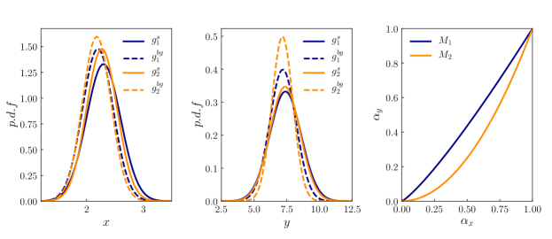
Figure 1: Signal and background distributions (continuous and dashed lines) predicted from $M_{1}$ (blue) and $M_{2}$ orange for the two experiments: $\text{E}_{\text{X}}$ in the left panel and $\text{E}_{\text{Y}}$ in the center. The fraction of the signal in $\text{E}_{\text{Y}}$ as a function of the signal in $\text{E}_{\text{X}}$ is shown in the right panel for the two models.

The signal and background are normal distributions (denoted by $g^{s}$ and $g^{bg}$ respectively) for the two models with the following parameters:

$$M_{1}\begin{cases}g_{1}^{s}(x)\text{ : }\mu=2.3\text{ and }\sigma=0.3\\ g_{1}^{bg}(x)\text{ : }\mu=2.2\text{ and }\sigma=0.27\\ g_{1}^{s}(y)\text{ : }\mu=7.4\text{ and }\sigma=1.2\\ g_{1}^{bg}(y)\text{ : }\mu=7.2\text{ and }\sigma=1\\ \end{cases}M_{2}\begin{cases}g_{2}^{s}(x)\text{ : }\mu=2.27\text{ and }\sigma=0.27\\ g_{2}^{bg}(x)\text{ : }\mu=2.18\text{ and }\sigma=0.25\\ g_{2}^{s}(y)\text{ : }\mu=7.37\text{ and }\sigma=1.15\\ g_{2}^{bg}(y)\text{ : }\mu=7.17\text{ and }\sigma=0.8\\ \end{cases}$$ (16)

We simulate two data samples (one for each experiment) following the model $M_{1}$ with $\alpha_{x}^{true}=0.3$. $\text{E}_{\text{X}}$ measures 300 events and $\text{E}_{\text{Y}}$ measures 200 events. For these simulations we have $\left\langle x\right\rangle=2.23$ and $\sigma_{x}=0.3$; $\left\langle y\right\rangle=7.27$ and $\sigma_{y}=1.07$. The likelihood function for the model $M_{i}$ ($i=1,2$) and variable $z$ ($z=x,y$) is given by:

$$f(z|\alpha_{z},M_{i})=\alpha_{z}g_{i}^{s}(z)+(1-\alpha_{z})g_{i}^{bg}(z).$$ (17)

Now we perform two analyses: one where each experiment analyse the data without any kind of information (Sec. 3.1) and another one where the experiments use the information obtained from the other (Sec. 3.2).

3.1 Independent analyses

In this approach the experiments have no any prior information but they are interested in the fraction of the signal, then the fraction of signal plus the fraction of background must be one. For this reason, each experiment choose a uniform distribution between $0$ and $1$ as its prior.

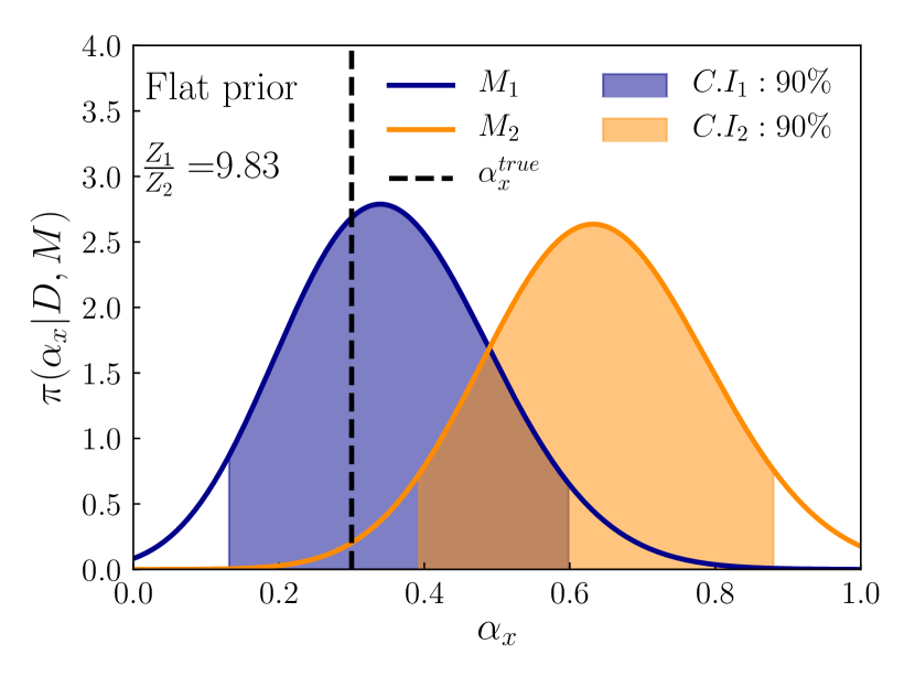
(a)

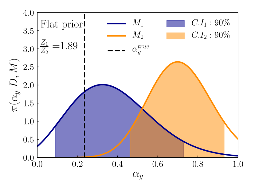
(b)

Figure 2: Posterior probability distributions of $\text{E}_{\text{X}}$ (a) and $\text{E}_{\text{Y}}$ (b) for the fraction of the interesting signal assuming the different models: $M_{1}$ (blue) and $M_{2}$ (orange).

In Fig. 2 the posterior probabiltiy distributions of the signals for each experiment under the assumption of the different models are displayed. We obtain numerically that $\text{E}_{\text{X}}$ obtains $\left\langle\alpha\right\rangle_{x}=0.33$ and a C.I at $90\%$ $[0.13,0.6]$ assuming $M_{1}$ while assuming $M_{1}$ $\text{E}_{\text{X}}$ obtains $\left\langle\alpha\right\rangle_{x}=0.6$ and $[0.4,0.9]$ as the posterior mean value of the fraction of the signal and C.I respectively. $\text{E}_{\text{Y}}$ obtains $\left\langle\alpha\right\rangle_{y}=0.38$ and C.I $0.09,0.74$ assuming $M_{1}$ and $\left\langle\alpha\right\rangle_{y}=0.62$ as fraction of the interesting signal with $[0.46,0.93]$ as a C.I assuming $M_{2}$. Since each experiment assumes $P(M_{1})=P(M_{2})=0.5$, before the analysis, $\text{E}_{\text{X}}$ arrives to the conclusion that $M_{1}$ is almost ten times most probable than $M_{2}$ while the resolution to discriminate between the models in $\text{E}_{\text{Y}}$ is smaller and for this experiment $P(M_{1}|D)/P(M_{1}|D)\sim 2$.

3.2 Combined analyses

When one experiment has analysed some data, its prior knowledge change, and these change can be use for the same experiment to analyse new data or for another experiment. In this example we show how the results of each experiment is used by the other. Assuming the results of $\text{E}_{\text{X}}$ in the previous section $\text{E}_{\text{Y}}$ can modify the prior of $\alpha_{y}$ for each theoretical model or scenario. In the same way, $\text{E}_{\text{X}}$ can do the same in sight of the analysis done by $\text{E}_{\text{Y}}$ . These new priors are shown together with the new results in Fig. 3.

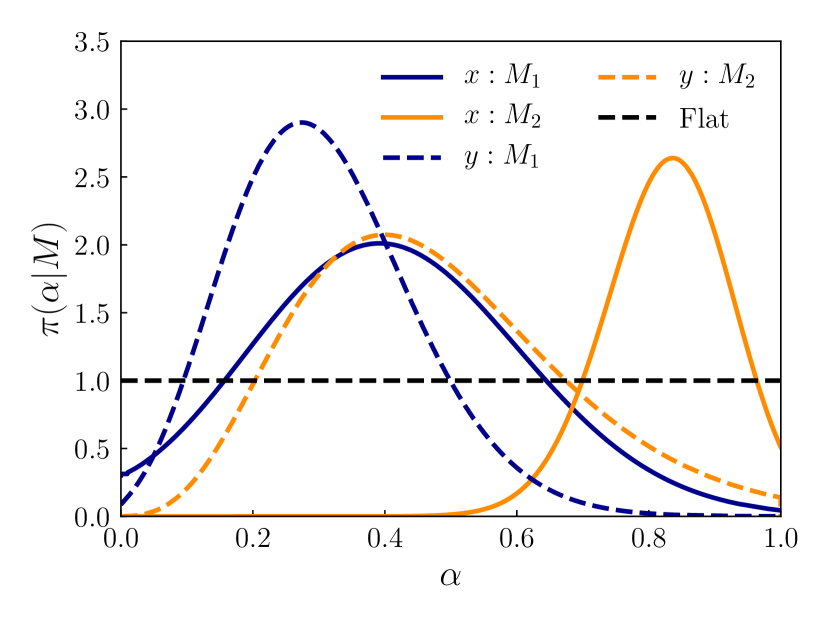
(a)

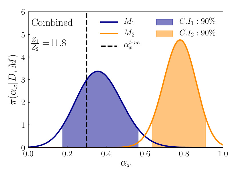
(b)

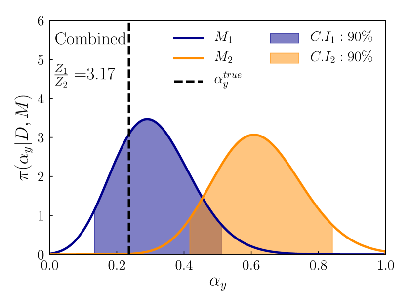
(c)

Figure 3: Prior probabilities for the signals given the independent analysis in panel (a): prior for $\alpha_{x}$ given the results of $\text{E}_{\text{Y}}$ assuming $M_{1}$ ($M_{2}$) is shown as continuous blue (orange) line; prior for $\alpha_{y}$ given the results of $\text{E}_{\text{X}}$ assuming $M_{1}$ ($M_{2}$) are shown as dashed blue (orange) line. They are compared with the uniform prior taken in the independent analysis (black dashed line). The posterior distributions for each experiment are shown in panels (b) and (c) for $\text{E}_{\text{X}}$ and $\text{E}_{\text{Y}}$ respectively.

One can observe that by including the results of one experiment in the other the results change. Now $\text{E}_{\text{X}}$ obtains that the posterior odds in favour of $M_{1}$ are: $P(M_{1}|D)/P(M_{2}|D)=11.8\times 1.89\approx 22$, increasing the evidence in favour of the model $M_{1}$. When $\text{E}_{\text{Y}}$ analyse its data taking into account the results of $\text{E}_{\text{X}}$ the posterior odds also increase being now $P(M_{1}|D)/P(M_{2}|D)\approx 31$. Therefore both experiments have reasons to beleave that the true model is $M_{1}$ and the joined results will be $\left\langle\alpha_{x}\right\rangle=0.36$ and $\left\langle\alpha_{y}\right\rangle=0.31$ with C.I $[0.18,0.56]$ and $[0.13,0.51]$ respectively being $M_{1}$ at least $22$ times more probable than $M_{2}$.

Finally, the posterior predictive distributions taking the results of the combined analysis are shown in Fig. 4. Even though the data can be well described by the two models, the Bayesian combined analysis permits us distinguish numerically between the two models.

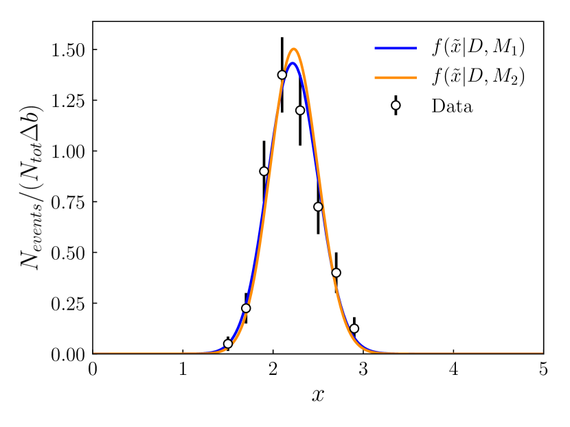
(a)

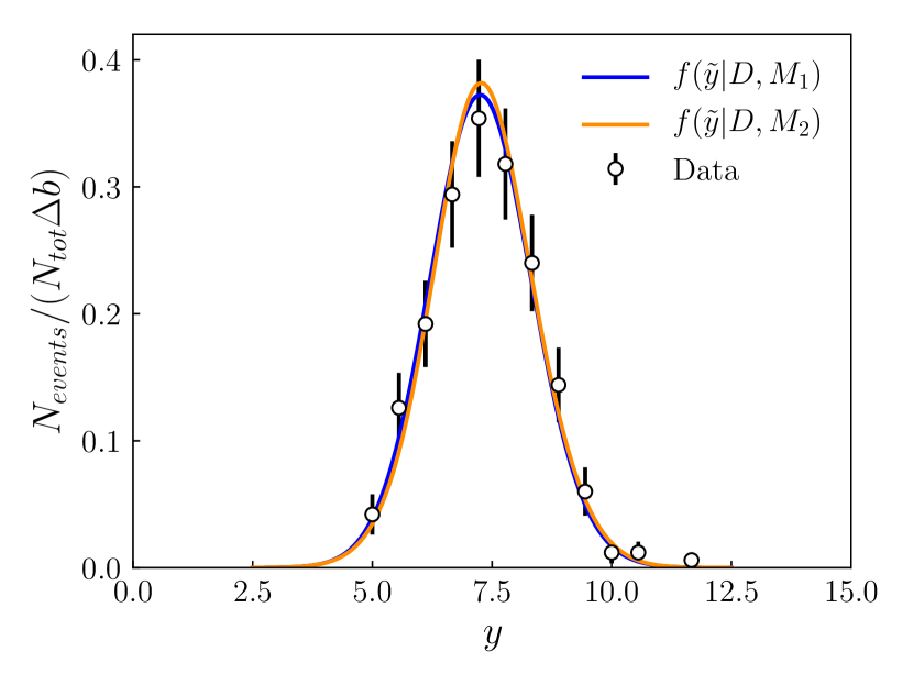
(b)

Figure 4: Posterior predictive distributions for $\text{E}_{\text{X}}$ (a) and $\text{E}_{\text{Y}}$ (b) compared with the observed data.

4 Conclusions

The Bayesian approach for the combination of different measurements and detectors has been presented and tested using simulations. With these methods the estimation of the parameters of interest and the discrimination among different theoretical models or scenarios can be improved using past or present experimental results from different experiments.

In this work we show how the combination of the information obtained with two different detectors can improve the parameter estimation, reduce the uncertainty and distinguish between theoretical models that can explain the same data.

References

- [1] Pierre Auger Collaboration, https://www.auger.org/
- [2] Telescope Array Project, www.telescopearray.org/
- [3] The High-Altitude Water Cherenkov Gamma-Ray Observatory, http://www.hawc-observatory.org/
- [4] IceCube Neutrino Observatory, https://icecube.wisc.edu/
- [5] MAGIC Collaboration, https://magic.mpp.mpg.de/
- [6] ANTARES Collaboration, http://antares.in2p3.fr/
- [7] Cherenkov Telescope Array, https://www.cta-observatory.org/
- [8] ANTARES Collaboration, http://antares.in2p3.fr/
- [9] KM3Net Collaboration, https://www.km3net.org/
- [10] J. O. Berger, R. L. Wolpert, M. J. Bayarri, M. H. DeGroot, B. M. Hill, D. A. Lane and L. LeCam The Likelihood Principle, IMS Lecture Notes–Monograph Series (1988) Institute of Mathematical Statistics
- [11] A. Brihnbaum, On the foundations of statistical inference, Journal of the American Statistical Association,57 (1962)