Trajectory stability in the traveling salesman problem

Abstract

Two generalizations of the traveling salesman problem in which sites change their position in time are presented. The way the rank of different trajectory lengths changes in time is studied using the rank diversity. We analyze the statistical properties of rank distributions and rank dynamics and give evidence that the shortest and longest trajectories are more predictable and robust to change, that is, more stable.

Introduction

Imagine that a certain product must be delivered, in the most efficient way, to $N$ stores in a region. When stores are fixed at given sites in space, finding the shortest path that links them all is the target of the traveling salesman problem (TSP) [1, 2], which here we refer to as static TSP. But what happens if the product must be delivered to moving targets such as peddlers? The TSP becomes time dependent. Another variation of the TSP, related to the peddlers’ scenario, occurs when one or more sites disappear and then reappear at other locations. Imagine, for example, a monkey looking for fruits that grow in a set of trees. What happens if one of the trees ceases producing fruits? The monkey, then, has to look for another tree. Time-dependent TSPs of this sort have several real-world applications, such as vehicle routing [3] and machine scheduling problems [4].

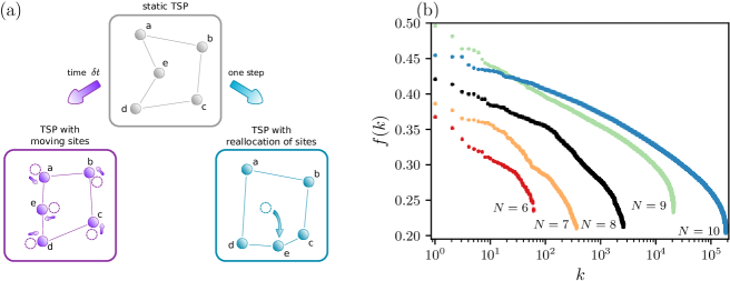
Figure 1: Time-dependent traveling salesman problem with moving sites and with reallocation of sites. Rank distribution for the TSP. (a) Diagram showing the two generalizations of the TSP considered here. By allowing nodes to shift in time, the static TSP (center) becomes time dependent. In the TSP with moving sites (left), these are displaced in a small interval $\delta t$. In the TSP with reallocation of sites (right), they are displaced to random positions after one time step. In these TSP variations, nodes do not move during path traversals, that is, the optimization problem of finding paths is solved for a static situation. Shortest paths are shown with lines between sites. (b) Rank distribution according to the inverse path length $f(k)$, for $N=6$ to $N=10$ sites in particular but representative instances of the TSP.

Many variations of the TSP have been analyzed in recent decades [1, 2]. Previous research related to the TSP has focused mainly on producing algorithms to find shortest paths but, to our knowledge, the properties of longer trajectories have not been discussed. In the present work we study the statistical properties of all trajectories in two generalizations of the TSP with time-dependent sites: the TSP with moving sites (bTSP), where sites can be interpreted as ‘boats’ that move gradually in a region, and the TSP with reallocation of sites (rTSP), where sites move discontinuously across space [Figure 1(a)]. In the peddlers’ example above, peddlers might not move during one day (so trajectories do not change) but on the next they may have a different position (possibly modifying the shortest path, such that a new optimization process is needed to find it). That would be equivalent to assume that trajectory changes in time-dependent TSPs occur at a much slower time scale than the traversal of the paths by salesmen. If we rank trajectories by their length, we can analyze how the properties of this ranking change in time with measures commonly used in the study of hierarchy dynamics in complex systems, such as the rank distribution $f(k)$ and the rank diversity $d(k)$ [5, 6].

Since the rank distribution was popularized in the 1930s by Zipf [7], it has been used to characterize complex systems of different nature [8]. We have recently discussed the cases of six indo-european languages [5] and of six sports and games [6], where we found that $f(k)$ does not follow Zipf’s law and varies slightly across cases. For all of these complex systems, we also studied how ranks change in time by means of the rank diversity $d(k)$. Explicitly, $d(k)$ is the number of different elements that have rank $k$ within a given period of time $T$. In the complex systems we have studied up until now, the rank diversity can be well approximated by a sigmoid curve.

Results

Static and time-dependent TSPs

Consider the static TSP with $N$ sites. We shall label each site by a, b, c, and so on. A trajectory is a closed path on these sites, so each trajectory can characterized by a non-unique string of site labels. For example, the shortest trajectory in Figure 1(a) for the static TSP (top) is “aedcb”. Note that one could have started the string at any site, and even changed the direction, so the same trajectory could have been labeled “cdeab”. Starting from his home city the salesman visits each site only once and returns home, that is, he follows a trajectory. There are $(N-1)!/2$ different trajectories, and the usual problem is to find the shortest one within this set. In this work we go further and rank each trajectory according to its length, so the shortest one has the highest rank ($k=1$), and the longest has the lowest rank ($k=k_{\max}=(N-1)!/2$). To study the rank distribution of the system, $f(k)$ is taken as the inverse of trajectory length. The rank distribution of TSP trajectories is presented in Figure 1(b) for several random configurations corresponding to different values of $N$. The results differ from Zipf’s law, but for all cases they have a similar shape, which resembles a beta distribution.

We now study the problem of stability of trajectories in the TSP. Suppose the location of sites varies slowly over time, so that the salesman can assume a static scenario for each travel, but the shortest trajectory, and in fact the rank of all trajectories, might change if the configuration of sites is modified enough. A toy model that captures this situation is the bTSP. Assume all $N$ sites are allowed to move within a $1\times 1$ square as if they were boats. In the TSP with moving sites, the $X$ and $Y$ components of the velocity of each site are random with a uniform distribution between $\pm 1$. The boats move with a constant velocity until they reach a confining wall, where they bounce elastically [see Figure 1(a) and accompanying video in Supplementary Information].

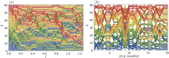
Figure 2: Time dependence of trajectory ranks. Time dependence of trajectory ranks for the models depicted in Figure 1(a), where particular instances of $N=6$ are considered. Colors are an aid to see how initial trajectory ranks diffuse over the $k$ axis as time goes by. We show results for the (a) bTSP, where trajectories spread slowly in time, and for the (b) TSP with reallocation of sites [rTSP], where there are drastic changes from one time step to another, as well as a tendency for keeping initially shorter/longer trajectories short/long.

Let us consider a different time-dependent perturbation of the TSP, the rTSP. Here $N$ sites are located in the unit square with a uniform random probability, and all trajectories are ranked as explained above. This is the “base” configuration. Then one site is chosen at random and reallocated to a random position in the unit square, after which trajectory ranks are calculated again [Figure 1(a)]. After several iterations, we can explore this time-dependent process with the rank diversity. Even though a continuous time dynamics does not exist as in the bTSP, we can still ask how many different trajectories occupy a given rank $k$, so the rank diversity is well defined.

Temporal evolution of trajectory ranks

We first explore how trajectory ranks change with time in both the bTSP and rTSP (Figure 2). For the bTSP, trajectories initially at the extremes (i.e. high or low $k$) tend to remain in place, until at some point they detach and explore a wider range of ranks [Figure 2(a)]. That is, in the edges of the plot (high and low $k$), rank as a function of $k$ tends to be a horizontal straight line, whereas for middle $k$ the corresponding lines vary more. For the rTSP a slightly different behavior is observed [Figure 2(b)]. Here we note that time is an auxiliary variable with no relevant meaning, since we are simply selecting random positions to relocate randomly chosen sites. As these positions are taken as a series of random and uncorrelated values, reordering such a sequence in time makes no statistical difference. Thus, it is reasonable to expect that trajectory ranks for the rTSP vary more than for the bTSP. Despite this fact, we also observe that the trajectories near the extremes tend to keep the same values of $k$, while intermediate trajectories do not exhibit such regularity, just like in the bTSP.

In order to quantify the way in which trajectory ranks change in time, we shall use the rank diversity. Moreover, to develop some intuition on this measure and understand how it depends on the parameters chosen to calculate it, we present several numerical experiments for both models in Figure 3. Note that to calculate the rank diversity we have to choose an appropriate time span $T$ and a number $m$ of time points at which observations are made. Alternatively, the time interval $\delta t$ between observations can be chosen instead of $m$, where $T=m\delta t$. In many real-world systems the time interval $\delta t$ is determined by data availability; to calculate the diversity of words in English throughout the centuries, for example, one may use Google’s n-gram dataset, which implies a time interval $\delta t$ of one year (or an integer multiple of that). However, in the bTSP both the total time $T$ and the time interval $\delta t$ can be chosen at will.

Let us analyze the situations depicted in Figure 3. First, we study the bTSP with a fixed total time evolution $T$ and varying $m$, thus effectively changing the value of $\delta t=T/m$ [Figure 3(a)]. As $m$ increases, the time between observations decreases, and the boats move less, so the positions of the boats barely change in a single time interval $\delta t$, and rank diversity diminishes. In fact, the diversity cannot be larger than the maximum number of trajectories divided by the number of time slots, $k_{\max}/m$. If, on the other hand, $m$ is small enough, $k_{\max}/m$ is larger than 1 and $d(k)$ tends to saturate around 1. This can be summarized in the formula

$$d_{\max}=\min\left\{1,\frac{(N-1)!}{2m}\right\}.$$ (1)

In the second scenario, we fix the number of observations and vary the total time $T$. As a limiting case, when $T$ is much larger than the time a boat needs to travel from one wall to another, the correlation between site configurations is lost, so for most ranks diversity is close to its maximum; only close to the shortest and longest trajectories we observe smaller diversities [Figure 3(b)]. Since both $N$ and $m$ are fixed, in this case $d_{\max}$ is the same for all $T$ values. We also analyze the case of a fixed value of $\delta t$ . The value of $m$ now changes, as in Figure 3(a), but simultaneously $T$ varies, as in Figure 3(b), due to the relation $\delta t=T/m$. As $m$ increases, the effect on diversity seems similar to the one in which $T$ is constant [Figure 3(c)]. Finally, we perform a similar analysis for the rTSP [Figure 3(d)]. As $m$ increases, the time between observations is not shortened. Each new position of the selected site is uncorrelated with the previous one, regardless of the value of $m$. We thus expect and observe a similar effect as the one of Figure 3(c). In this case, the bound for different values of $m$ does not change, since $(N-1)!/2m>1$ for all cases shown.

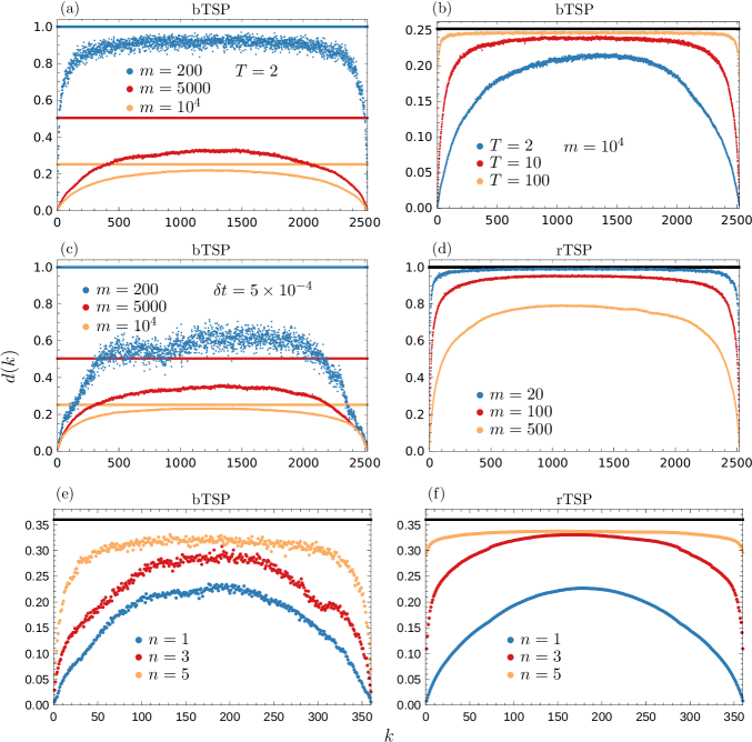
Figure 3: Parameter dependence of rank diversity. We analyze how changing parameter values affects the rank diversity for two time-dependent versions of the TSP. For panels (a)-(d) we consider $N=8$. Starting with the bTSP and $n=N$, we: (a) vary the number of observations $m$ while keeping the total time $T=2$; (b) fix the number of time steps $m=10^{4}$ while varying the total time; and (c) fix the value of $\delta t=5\times 10^{-4}$ while changing the number of time steps (and thus the total time). For the rTSP, we also (d) show how changing the number of time steps alters the diversity. Curves are averages over 100 realizations. Panels (e) and (f) respectively show the rank diversity for the bTSP when $n$ sites are allowed to move, and for the rTSP when $n$ sites are reallocated at each time step, both with $N=7$ and $m=1000$. For the bTSP the total time is $T=10$, which leads to $\delta t=0.1$. We choose this value of $T$ so that (e) and (f) resemble each other. Results in (f) are averages over 1000 realizations. Horizontal lines correspond to $d_{\max}$, the maximum value of the diversity given in Eq. (1). In (b), (d), (e) and (f) all curves have the same bound, whereas in (a) and (c) color is used to indicate the bounds of each curve.

Two useful generalizations of the bTSP and the rTSP are now considered, since it will allow us to relate the behavior of both models. Assume that only some sites move in the bTSP. That is, instead of all site moving in the plane, $n$ move and $N-n$ are static. The cases analyzed before thus correspond to $n=N$. In a similar way, consider an rTSP where instead of reallocating a single site, $n$ sites are moved. The case $n=N$ thus corresponds to a total reallocation of the system, while up to now we have only discussed the value $n=1$. Diversity for these generalizations seems to behave in a similar way as for the case $n=1$, as seen in Figure 3(e) and Figure 3(f). In fact, for the bTSP one may even consider a single moving site and the previous conclusions still hold. We have obtained similar results for other variations of the bTSP, such as periodic boundary conditions, and different ways of choosing the initial conditions and velocities.

Let us analyze geometrically a particular, but random, instance of the rTSP with the goal of gaining some insight. The configuration space of such problem has dimension $2n$, as each of the $n$ sites has a two dimensional space to move. For a given initial configuration, in the case $n=1$ we can plot the locus of positions to which a given point may travel, so the trajectory associated with a given rank remains unchanged. In Figures 4(a-c) we take $N=7$ as an example, so the shortest, middle and longest trajectories correspond to $k=1,k=180$, and $k=360$, respectively. The example is representative in the sense that, for the extremal trajectories, the aforementioned locus has a big area and the middle one has a very small area, but particular values change broadly from realization to realization. We can also obtain a histogram of the probability density $\rho_{k}$ of the areas corresponding to random realizations [Figure 4(d-f)]. From these histograms we see that $\rho_{1}\approx\rho_{k_{\max}}$, but $\rho_{1}$ is clearly different from $\rho_{k_{\max}/2}$.

It is also useful to study the expected value of the stability area for different ranks, $\langle A\rangle_{\rho_{k}}$, as a function of the number of sites (Figure 5). There is a different scaling for the extremal and intermediate rankings, so we expect that the difference in areas seen for the case $N=7$ is exponentially larger for bigger systems. Although the standard deviation of the distribution $\rho_{k}$ is relatively large, the average value $\langle A\rangle_{\rho_{k}}$ can be determined with high accuracy (the statistical error for points in Figure 5 are comparable to the size of the points). We can also see an even-odd effect for the longest trajectory associated with the change in topology of a star-like configuration for an even or odd number of sites. This hints at a geometric understanding of time-dependent TSPs which, however, is outside the scope of the present study.

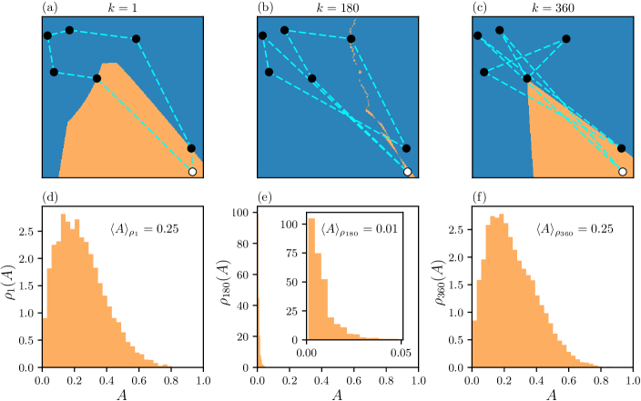
Figure 4: Stability of ranks under reallocation of sites. (a) Particular instance of the rTSP with $N=7$ and $n=1$. Black points represent fixed sites, whereas the white one represents the site to be reallocated. The shortest trajectory is indicated as a dashed red line. When the white point is reallocated in the green area $A$, the shortest trajectory remains unchanged, while if a node is reallocated in any part of the blue area, the shortest trajectory changes. (b) Same realization of the rTSP, but for the trajectory with an intermediate rank ($k=180$). The green area is much smaller in this case. (c) Same realization of the rTSP, but for the longest trajectory ($k=360$), where the green area is again big. In panels (d), (e) and (f) we show the probability distributions of $A$ for $N=7$ and the three previous values of $k$, as well as its mean value, $\langle A\rangle_{\rho_{k}}$.

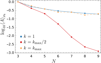
Figure 5: Scaling in rank stability. Scaling of the average value of the area for which a change in position will not change the rank of a trajectory, for ranks $k=1$, $k_{\max}/2$ and $k_{\max}$, and for different system sizes.

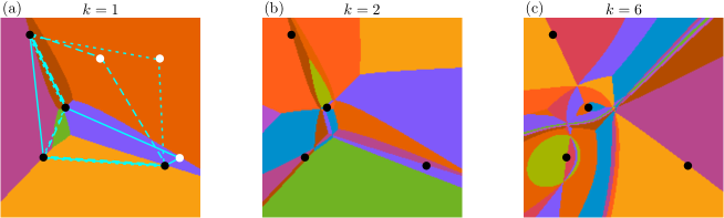
Figure 6: Stability areas for different trajectories. (a) rTSP with $N=5$, $n=1$, and three possible reallocations of the white point. The shortest trajectory, $k=1$, is indicated as a solid, dashed and dotted line, corresponding to the three reallocations. Regions of varying color correspond to different trajectories for $k=1$ (see Figure 4, top row). In panels (b) and (c) we show a plot with the same fixed sites as in (a), but for $k=2$ and $k=6$, respectively.

Connecting the bTSP and rTSP

Consider the rTSP with $n=1$. For a particular rank $k$, each position in the unit square yields a trajectory. We can thus ‘paint’ the unit square with colors corresponding to trajectories. We show examples with $N=5$ for the shortest trajectory in Figure 6(a), and for $k=2$ and $6$ in Figure 6(b) and Figure 6(c), respectively. Diversity is the number of different colors in the picture divided by the number of observations. Notice that there is a qualitative difference between the cases $k=1$ and $k=6$. This indicates already that $d(1)<d(6)$ if a large ensemble is taken (so that errors due to finite sampling are small enough).

For the bTSP with $n=1$, the moving boat will cover the whole unit square uniformly for most choices of the velocities. The condition for having a uniform covering is that the vertical and horizontal speeds are incommensurable, which always holds for this model. When this occurs, time averages yield the same value as space averages, i.e., the system is ergodic [9]. For such long times the whole unit square will be visited, i.e. the moving site will visit all colored areas. Therefore, the bTSP has the same rank diversity as the rTSP when the sampling $m$ is the same (otherwise they are related by a constant factor).

For a larger number of moving sites, $n>1$, a similar reasoning holds. However, the configuration space is now $2n$ dimensional, and thus visualizing it is more challenging. The condition for ergodicity still holds when all pairs of velocities are incommensurable. However, when the number of boats that move is increased, the diversity changes as in Figure 3(e) (where three different values of $n$ are shown). When $n=N-1$ or $N$, the diversity is formally maximum and we obtain no relevant information. In fact, when the time over which we calculate the diversity in the bTSP increases, $d(k)$ tends to 1 [Figure 3(b)].

The bTSP and rTSP are comparable since both explore a fraction of the $2N$-dimensional configuration space. The bTSP explores a line of finite length in such a space, or a $2N$ dimensional hypercube embedded in the configuration space if the whole ensemble of velocities is considered. The rTSP, on the other hand, explores a $2n$ dimensional hyperplane embedded in the same configuration space. Overall, both models behave in a similar fashion.

Each realization of the TSP can be seen as a point in a $2N$-dimensional configuration space, where every pair of axis defines the coordinates of each particle. The optimization problem is then different for each point in the configuration space. We have analyzed the stability of the solutions of the TSP under changes of the location of the point defining the configuration. We have further shown that the stability properties are similar for the two time-dependent generalizations of the TSP considered here. We have also stated under what conditions the behavior of both models is identical. We thus expect that these results are applicable to other perturbations of the TSP that involve small variations in configuration space.

Discussion

We have studied the statistical properties of rank distributions and rank dynamics of a novel variation of the traveling salesman problem where nodes shift their position in time. This allows us to explore the stability of trajectory ranking, which is related to the predictability of perturbation effects. Figure 5 shows the average probability of a trajectory maintaining its rank of 1000 instances of the bTSP (with one site moving) as the number $N$ of sites increases. We see that this probability, which reflects the stability of ranks to perturbations, decreases with $N$. However, the decrease is much lower for the shortest and longest paths than for the middle trajectories. This reflects the fact that the rank diversity is also lowest for the extreme paths. Moreover, the stability decreases much faster for the middle trajectories. Thus, we find that the shortest and longest trajectories are more predictable and robust. This claim would benefit from analytic solutions for the numerical results presented here, but these are beyond the scope of the present work.

We also note that rank diversity curves are all symmetric, as shown in Figure 3. However, in previous studies we have shown that the rank diversity $d(k)$ has almost the same form for languages, sports and games. This is not symmetric and can be adjusted by a sigmoid in lognormal scale. Still, from other datasets we have also noticed symmetric rank diversity curves. The difference between symmetric and non-symmetric rank diversity curves seems to be related with the degree of ‘openness’ of a system. In time-dependent TSPs the system is ‘closed’, as all trajectories are considered at all times. However, in sports, languages and other real-world phenomena, elements enter and exit the system. More precisely, elements enter and exit the subset of the system available in datasets. If one plots rank diversity curves of ‘open’ systems in linear scale, they are very similar to the symmetric curves of closed systems [5, 6].

Changes in optimization problems pose challenges when change is faster than optimization, as solutions might be obsolete [10]. These non-stationary problems are a common feature of complex systems [11]. Our analysis suggests that the way in which state spaces of non-stationary problems change is not uniform. This implies that once an optimal solution is found, we can expect it to be more stable than non-optimal solutions. A more detailed exploration of the changes of state spaces in time will provide further insight, and we trust that the methods presented here will contribute to this effort.

Data Availability

The datasets generated during and/or analyzed during the current study are available from the corresponding author on reasonable request.

Author contributions statement

J.F. and C.P. conceived the ideas behind this work. G.C. obtained the rank distribution for the static TSP. S.S. and C.P. carried out the numerical simulations and statistical tests. G.I. provided the framework to contextualize the results. J.F., C.P., G.I., and C.G. wrote the manuscript. All authors discussed and reviewed the manuscript.

Additional information

Competing financial interests
The authors declare that they have no competing interests.

References

- [1] Lawler, E. L., Lenstra, J. K. & Rinnooy Kan, A. H. The traveling salesman problem (1985).
- [2] Gutin, G. & Punnen, A. The Traveling Salesman Problem and Its Variations. Combinatorial Optimization (Springer US, 2007). URL https://books.google.com.mx/books?id=pfRSPwAACAAJ.
- [3] Malandraki, C. & Daskin, M. S. Time dependent vehicle routing problems: Formulations, properties and heuristic algorithms. Transportation science 26, 185–200 (1992).
- [4] Bigras, L.-P., Gamache, M. & Savard, G. The time-dependent traveling salesman problem and single machine scheduling problems with sequence dependent setup times. Discrete Optimization 5, 685 – 699 (2008). URL http://www.sciencedirect.com/science/article/pii/S1572528608000339. DOI http://doi.org/10.1016/j.disopt.2008.04.001.
- [5] Cocho, G., Flores, J., Gershenson, C., Pineda, C. & Sánchez, S. Rank diversity of languages: Generic behavior in computational linguistics. PLoS ONE 10, e0121898 (2015). URL http://dx.doi.org/10.1371%2Fjournal.pone.0121898. DOI 10.1371/journal.pone.0121898.
- [6] Morales, J. A. et al. Generic temporal features of performance rankings in sports and games. EPJ Data Science 5, 33 (2016). URL http://dx.doi.org/10.1140/epjds/s13688-016-0096-y. DOI 10.1140/epjds/s13688-016-0096-y.
- [7] Zipf, G. K. Selective Studies and the Principle of Relative Frequency in Language (Harvard University Press, Cambridge, MA, USA, 1932).
- [8] Clauset, A., Shalizi, C. R. & Newman, M. E. Power-law distributions in empirical data. SIAM Review 51, 661–703 (2009).
- [9] Yaglom, A. M. An introduction to the theory of stationary random functions. (Prentice-Hall, Inc., New Jersey., 1962).
- [10] Gershenson, C. Facing complexity: Prediction vs. adaptation. In Massip, A. & Bastardas, A. (eds.) Complexity Perspectives on Language, Communication and Society, 3–14 (Springer, Berlin Heidelberg, 2013). URL http://arxiv.org/abs/1112.3843.
- [11] Gershenson, C. The implications of interactions for science and philosophy. Foundations of Science 18, 781–790 (2013). URL http://arxiv.org/abs/1105.2827. DOI 10.1007/s10699-012-9305-8.
Acknowledgements
We acknowledge support from UNAM-PAPIIT Grant No. IN111015.