Hyperbolic Covariant Coherent Structures in two dimensional flows

Abstract

A new method to describe hyperbolic patterns in two dimensional flows is proposed. The method is based on the Covariant Lyapunov Vectors (CLVs), which have the properties to be covariant with the dynamics, and thus being mapped by the tangent linear operator into another CLVs basis, they are norm independent, invariant under time reversal and can be not orthonormal. CLVs can thus give a more detailed information on the expansion and contraction directions of the flow than the Lyapunov Vector bases, that are instead always orthogonal. We suggest a definition of Hyperbolic Covariant Coherent Structures (HCCSs), that can be defined on the scalar field representing the angle between the CLVs. HCCSs can be defined for every time instant and could be useful to understand the long term behaviour of particle tracers. We consider three examples: a simple autonomous Hamiltonian system, as well as the non-autonomous “double gyre” and Bickley jet, to see how well the angle is able to describe particular patterns and barriers. We compare the results from the HCCSs with other coherent patterns defined on finite time by the Finite Time Lyapunov Exponents (FTLEs), to see how the behaviour of these structures change asymptotically.

I Introduction

In the paradigm of chaotic advection, the trajectories of passive tracers can be complex even when the velocity field of the flow is simple. This is the case, for example, for time dependent two-dimensional flows or even steady three-dimensional flows, like the celebrated ABC flow Dombre et al. (1986). However, even flows with complicated time dependent structure allow for the formation of coherent patterns that influence the evolution of tracers. These structures are common in nature, appearing both at short and long time scales as well as small and large spatial scales. Remarkable examples of these structures are eddies and jets in the ocean and atmosphere, the Gulf Stream current, and ring clouds Haller (2015). These patterns can influence, for example, the evolution of nutrients as well as oil spills and other pollutants. Furthermore, these coherent structures could act as local inhibitor for the energy transfer between scales Kelley et al. (2013). They also appear in other planets and other astrophysical systems, such as the jets on the surface of Jupiter, Saturn and other gaseous planets, and in the solar photospheric flows Chian et al. (2014). These structures, often referred as Lagrangian Coherent Structures (LCSs), can shed light on the mixing and transport properties of a particular system on a finite time interval. The term “Lagrangian” in their name is motivated by the fact that they evolve as material lines with the flow Haller (2015). A particular kind of LCS is called Hyperbolic LCS (HLCS), and can be seen as the locally most attracting or repelling material lines that characterize the dynamical system over a finite time interval. The term hyperbolic is just an analogy with the stability of fixed points in dynamical systems, since usually one wants to study non-autonomous systems for which entities such as fixed points or stable and unstable manifolds are not defined. Moreover these systems are studied for finite time.

Early attempts to detect HLCSs were based on Finite Time Lyapunov Exponents (FTLEs), that measure the rate at which initial conditions (or, equivalently, tracer particles) separate locally after a given interval of timePierrehumbert and Yang (1993); Doerner et al. (1999); Haller and Yuan (2000); Haller (2001); Lapeyre (2002); Shadden et al. (2005); Lekien et al. (2007); Sulman et al. (2013). One of the first rigorous definitions of the LCSs was based on ridges of the FTLEs Shadden et al. (2005). FTLEs and the so defined LCSs were used to study for example Lagrangian dynamics of atmospheric jets Rypina et al. (2007) and oceanic stirring by mesoscale eddies Rypina et al. (2010); Beron-Vera et al. (2008); Waugh and Abraham (2008); Bettencourt et al. (2012); Harrison and Glatzmaier (2012); Waugh et al. (2012), describing for example the chaotic advection emerging by mixed layer instabilities and its sensitivity to the vertical shear Mukiibi et al. (2016). A similar method to detect coherent structures uses the Finite Size Lyapunov Exponents (FSLEs), that represents the separation rate of particles given a specific final distance Joseph and Legras (2002); d’Ovidio et al. (2004); Cencini and Vulpiani (2013). However, several counter examples are available in which both FTLEs and FSLEs ridges fail in characterizing the LCSs Karrasch and Haller (2013); Karrasch (2015). Although the FTLEs field remain a popular diagnostics of chaotic stirring, other methods now are available to detect LCSs, which include for example the so called Lagrangian descriptors Mancho et al. (2013); Lopesino et al. (2017), which are based on integration along trajectories, for a finite time, of an intrinsic bounded positive geometrical and/or physical property of the trajectories themselves. Notice however that the method of Lagrangian descriptors is not objective Vortmeyer-Kley et al. (2016); the connection between the Perron-Frobenius operator and almost invariant coherent sets of non-autonomous dynamical systems defined over infinite times Froyland et al. (2010), the use of braids Thiffeault (2010), and the extrema of trajectories Mundel et al. (2014). Other Fast Indicators (FIs) besides FTLEs and FSLEs, i.e. computational diagnostics that characterize chaos quickly and can be used to determine coherent structures, are the Smaller (SALI) and Generalized (GALI) Alignment Indices Skokos et al. (2007), the Mean Exponential Growth rate of Nearby Orbits (MEGNO) Cincotta and Simo (2000), and the Finite Time Rotation Number (FTRN) Szezech et al. (2013, 2012); Jr. et al. (2009).

Particularly promising for the detection of coherent structures is a variational theory that considers the extremum properties of a specific repulsion rate function Haller (2011); Farazmand and Haller (2012); Karrasch (2012); Farazmand and Haller (2012, 2013); Karrasch (2015); Blazevski and Haller (2014). Using this theory it has been further shown that HLCSs can be described using geodesics Haller and Beron-Vera (2012). In this way, HLCSs can be represented as minimizers of a material length, with specific boundary conditions for the variation function. Another geodesic theory describes HLCSs in terms of shearless transport barrier that minimize the average shear functional Farazmand and Haller (2013); Farazmand et al. (2014). These theories are based on the computation of shrink/stretch-lines (tensorlines), thus trajectories along the eigenvectors of the deformation tensor also called Cauchy Green Tensor (CGT). Geodesic theories are also able to detect other two kinds of LCSs called Parabolic and Elliptic, which are however of no interest for the present work.

All these methods such as FTLEs, FSLEs, or the variational and geodesic theories, aim to find particular structures on the flow, among these the most repelling, or attracting, structures in the flow on a finite time interval, the HLCS. Particle tracers around these most influential material structures in finite time are maximally repelled or attracted. However, changing the finite time interval under study also changes the dynamical system and the correspondent structures emerging from the flow. Recent effort has been done in the understanding the instantaneous most influential coherent structures, Objective Eulerian Coherent Structures (OECSs), using a method that is not based on a finite time interval of evolution Serra and Haller (2016, 2017a, 2017b). The tracer particles could be maximally repelled for a short time, but on long time they could have a different behaviour. Is it natural to wonder what happen asymptotically to the tracer particles? Is it possible to find some coherent structures that suggest the asymptotic behaviour of the tracer particles?

In this work we thus propose an alternative method to detect coherent patterns emerging in chaotic advection, which is based on the Covariant Lyapunov Vectors (CLVs). CLVs were first introduced by Oseledec Oseledec (1968) and Ruelle Ruelle (1979), but for a long time they have received very little attention due to the lack of an efficient algorithm to compute them. Only in the last decade the computation of such vectors has become possible Wolfe and Roger M. (2007); Ginelli et al. (2007); Fro (2013), and CLVs have been used to investigate e.g. the motion of rigid disk systems Bosetti and Posch (2010), convection Xu and Paul (2016), and other atmospheric phenomena Wolfe and Samelson (2008); Schubert and Lucarini (2015, 2016); Vannitsem and Lucarini . For other theoretical discussions or for reviews on CLVs, see e.g. Refs. Yang and Radons (2008, 2010); Kuptsov and Parlitz (2012); Sala et al. (2012); Ginelli et al. (2013). Unlike the Lyapunov Exponents (LEs), which are time independent, the correspondent vectors, also known as forward and backward Lyapunov Vectors (LVs), do depend on time. The LVs are orthonormal and their direction can thus give only limited information about the local structure of the attractor. LVs also depend on the chosen norm, they are not invariant under time inversion and they are not covariant, where covariance is here defined as the property of the forward (backward) LVs to be mapped by the tangent dynamics in forward (backward) LVs at the image point Kuptsov and Parlitz (2012). Differently from the LVs, CLVs are norm independent, invariant for temporal inversion and covariant with the dynamics, making them thus mapped by the tangent linear operator into another CLVs bases during the evolution of the system. They are not orthonormal and their directions can thus probe better the tangent structure of the system.

All this intrinsic information can be summarized using the angle between the CLVs, a scalar field that allows to investigate the spatial structures of the system. The need to pay more attention to the directions between LVs, backward and forward, has also been suggested for the study of turbulence Lapeyre (2002) and for the definition of a diagnostic quantity for the study of mixing, the Lyapunov’s diffusion d ’Ovidio et al. (2009). Using three simple examples, we show that the attracting and repelling barriers tend to align along the paths on which the CLVs are orthogonal. The directions of the CLVs along these maxima provide thus information on the attracting or repelling nature of the barriers and can be related to the geometry of the system. Using the CLVs we can define structures, at a given time instant, that are asymptotically the most attractive or repelling. Furthermore, since these structures can be defined for every time instant, it is possible to follow the formation of coherent structures during the evolution of the flow.

In section II we discuss the theory behind the CLVs, and suggest a definition for coherent structures that give asymptotic information. The strategy will be to make use of the scalar quantity defined by the angle between the CLVs to locally identify the structures that asymptotically are maximally attractive or repulsive. In section III we use the CLVs to identify particular patterns in three different systems and we compare the results with FTLEs fields. Finally, in section IV we summarize the conclusions.

II Covariant Lyapunov Vectors

In this section we summarize the theory behind CLVs for two dimensional flows. For a more general and detailed review see for example Ref. Kuptsov and Parlitz (2012). Let the open set $D\subset\mathbb{R}^{2}$ be the domain of the flow, $t\in\mathbb{R}$ the time and ${\bf v}({\bf x},t)$ a vector velocity field in $D$. The dynamical system that describes the motion of a tracer advected by the flow is thus

$$\frac{d{\bf x}({\bf x}_{0},t_{0};t)}{dt}={\bf v}({\bf x}({\bf x}_{0},t_{0};t),t),$$ (1a)

$${\bf x}({\bf x}_{0},t_{0};t_{0})={\bf x}_{0},$$ (1b)

where ${\bf x}({\bf x}_{0},t_{0},t)\in D$ is the trajectory of the tracer starting at the point ${\bf x}_{0}$ at time $t_{0}$. To (1) is associated the flow map $\bm{\phi}_{t_{0}}^{t}({\bf x}_{0})$

$$\begin{split}&\bm{\phi}_{t_{0}}^{t}:D\to D,\\ &{\bf x}_{0}\to{\bf x}({\bf x}_{0},t_{0},t),\end{split}$$ (2)

that maps the initial position ${\bf x}_{0}$ at time $t_{0}$ to the position ${\bf x}({\bf x}_{0},t_{0},t)$ at time $t$. It should be noted that the dependence on the initial condition is very important here, since the vectors will be considered as function of time and of the initial positions. In the following, the contracted form ${\bf x}={\bf x}({\bf x}_{0},t_{0},t)$ will be used.

At each point ${\bf x}\in D$ we can identify the tangent space $T_{{\bf x}}D\subset\mathbb{R}^{2}$. Infinitesimal perturbations, ${\bf u}(t)\in T_{{\bf x}}D$, to a trajectory of this system can be described by the linearized system

$$\frac{d{\bf u}(t)}{dt}={\bf J}(t)\,{\bf u}(t),$$ (3a)

$${\bf u}(t_{0})={\bf u}_{0},$$ (3b)

where ${\bf J}(t)\in\mathbb{R}^{2\times 2}$ is the Jacobian matrix composed by the derivatives of the vector field ${\bf v}({\bf x},t)$ with respect to the component of the vector ${\bf x}$. Using the fundamental matrix ${\bf M}(t)\in\mathbb{R}^{2\times 2}$, of (3), that satisfies

$$\frac{d{\bf M}(t)}{dt} = {\bf J}(t){\bf M}(t),$$ (4a)

$${\bf M}(0) = {\bf I}$$ (4b)

we define the so called tangent linear propagator

$${\bf F}(t_{0},t)={\bf M}(t){\bf M}(t_{0})^{-1}.$$ (5)

${\bf F}(t_{0},t)$ maps a vector in ${\bf x}_{0}$ at time $t_{0}$ into a vector in ${\bf x}$ at time $t$ along the same trajectory of the starting system (1), that is

$${\bf u}(t)={\bf F}(t_{0},t)\,{\bf u}(t_{0}).$$ (6)

According to (5), the propagator is always nonsingular. In terms of the flow map, the tangent linear propagator is

$${\bf F}(t_{0},t)=\nabla\bm{\phi}_{t_{0}}^{t}.$$ (7)

Exploiting Oseledec’s Theorem Oseledec (1968); Eckmann and Ruelle (1985), it is possible to characterize the system using quantities that are independent on $t$ or $t_{0}$. By virtue of this theorem the far-future operator

$${\bf O}^{+}(t_{0})=\lim_{t\to+\infty}\left({\bf F}(t_{0},t)^{\top}{\bf F}(t_{0},t)\right)^{1/2(t-t_{0})}$$ (8)

and the far-past operator

$${\bf O}^{-}(t)=\lim_{t_{0}\to-\infty}\left({\bf F}(t_{0},t)^{-\top}{\bf F}(t_{0},t)^{-1}\right)^{1/2(t-t_{0})}$$ (9)

are well defined quantities. Note that the product ${\bf F}^{\top}(t_{0},t){\bf F}(t_{0},t)$ determines the Euclidean norm of the tangent vectors in the forward-time dynamics (a similar role it is played by ${\bf F}^{-\top}(t_{0},t){\bf F}^{-1}(t_{0},t)$ for the backward-time dynamics), in fact,

$$\lvert\lvert{\bf u}(t)\rvert\rvert=\left[{\bf u}(t_{0})^{\top}\left({\bf F}^{\top}(t_{0},t){\bf F}(t_{0},t)\right){\bf u}(t_{0})\right]^{1/2}.$$ (10)

Operators (8) and (9) probe respectively the future and past dynamics of a certain point, and share the same eigenvalues

$$\lambda_{1}\geq\lambda_{2},$$ (11)

that, assuming ergodicity, are independent on time and space. Each eigenvalue has multiplicity $m_{i}$ ($m_{1}+m_{2}=2$). Their logarithms correspond to the LEs of the dynamical system (1). If the limits in (8) and (9) are not considered, the resulting eigenvalues are time and space dependent and are called FTLEs.

The two operators (8) and (9) can be evaluated at the same point in space at a given time $t$. The correspondent eigenvectors, $\{{\bf l}^{+}_{1}(t),\,\,{\bf l}^{+}_{2}(t)\}$, $\{{\bf l}^{-}_{1}(t),\,\,{\bf l}^{-}_{2}(t)\}$ will define thus the forward and backward Lyapunov basis computed at the same time. Conversely to the respective eigenvalues those bases are time dependent, depend on the chosen scalar product and are not invariant under time reversal. Furthermore, these vectors are always orthogonal and give thus limited information on the spatial structure of the configuration space.

To overcome these issues, one can build particular spaces, the backward and forward Oseledec subspaces, defined as Oseledec (1968)

$$L^{-}_{i}(t)=\text{span}\{{\bf l}^{-}_{j}(t)\lvert j=1,i\},\quad i=1,2,\quad L^{-}_{0}(t)=\emptyset,$$ (12)

and

$$L^{+}_{i}(t)=\text{span}\{{\bf l}^{+}_{j}(t)\lvert j=i,2\},\quad i=1,2,\quad L^{+}_{0}(t)=\emptyset$$ (13)

In the forward dynamics, the generic vector ${\bf l}^{+}_{i}(t)$ grows or decays exponentially with an average rate $\lambda_{i}$. If the system is evolved forward in time, by means of the tangent linear propagator the evolution of the vector ${\bf l}^{+}_{1}(t)$ will have a non-zero projection inside the space generated by ${\bf l}^{+}_{1}(t^{\prime})$, but it will also have a non-zero projection onto the space generated by ${\bf l}^{+}_{2}(t^{\prime})$. On the other hand, ${\bf l}^{+}_{2}(t)$ will be transported onto the space generated by ${\bf l}^{+}_{2}(t^{\prime})$ and will have zero projection onto the space generated by ${\bf l}^{+}_{1}(t^{\prime})$. Repeating similar arguments for the backward Lyapunov Vectors leads to the observation that $L^{-}_{i}$ and $L^{+}_{i}$ are covariant subspaces,

$$L^{-}_{i}(t^{\prime}) = {\bf F}(t,t^{\prime})L^{-}_{i}(t),$$ (14a)

$$L^{+}_{i}(t^{\prime}) = {\bf F}(t,t^{\prime})L^{+}_{i}(t).$$ (14b)

Vectors that are covariant with the dynamics and invariant with respect to time reversal will be found at the intersection of the Oseledec subspaces, i.e. at

$${\bf w}_{i}(t)=L^{-}_{i}(t)\cap L^{+}_{i}(t).$$ (15)

These spaces, often referred as Oseledec splitting Ruelle (1979); Oseledec (1968); Ginelli et al. (2007, 2013), are not empty Kuptsov and Parlitz (2012), and their vectors, also called covariant Lyapunov vectors (CLVs), are covariant with the dynamics, i.e.

$${\bf F}(t,t^{\prime}){\bf w}_{i}(t)={\bf w}_{i}(t^{\prime}).$$ (16)

It should be noted that CLVs posses thus the properties of a semi-group. These vectors have an asymptotic grow or decay with an average rate $\lambda_{i}$, so that their asymptotic behaviour can be summarized as

$$\lVert{\bf F}(t,t\pm\tau){\bf w}_{i}(t)\rVert\approx e^{\pm\lambda_{i}\tau},$$ (17)

where $\tau=\lvert t^{\prime}-t\rvert$, which shows their invariance under time reversal. Note also that these vectors do not depend on any particular norm.

Equations (12), (13) and (15) imply a simple relation between CLVs and LVs in a two dimensional system,

$${\bf w}_{1}\equiv{\bf l}^{-}_{1}\quad\text{and}\quad{\bf w}_{2}\equiv{\bf l}^{+}_{2},$$ (18)

the first CLV corresponds to the first backward Lyapunov vector, and the second CLV with the second forward Lyapunov vector.

Furthermore, if the Jacobian matrix appearing in (3) is constant, the CLVs are not just covariant, but invariant with the dynamics. In this particular case in fact they correspond to the eigenvectors of the Jacobian and the eigenvalues of this matrix coincide with the LEs.

Since the CLVs highlight particular expansion and contraction directions at each point of the coordinate space, and these directions are not necessarily orthogonal, they can be used to understand the geometrical structure of the tangent space. This geometric information can be summarized by the scalar field of the angle $\theta(t)$ between the CLVs. Because the CLVs identify asymptotically the expansion and contraction directions sets of the tangent space associated at every point of the domain, the $\theta$ field represents a measure of the hyperbolicity of the system, that is a measure of the orthogonality between these two directions. Note that the orientation of the CLVs is defined as arbitrary. The angle between the CLVs,

$$\theta(t)\in\left[0,\,\,\frac{\pi}{2}\right],$$ (19)

is thus

$$\theta(t)=\cos^{-1}\left(\lvert{\bf w}_{1}(t)\cdot{\bf w}_{2}(t)\lvert\right),$$ (20)

where $\{{\bf w}_{1}(t),\,{\bf w}_{2}(t)\}$ are the first and the second CLVs Ginelli et al. (2007). It is interesting to point out that when $\theta(t)=\pi/2$, the CLVs reduce to LVs in two dimensions, and the backward and forward Lyapunov basis coincide. If the computation of the angle is done at every point of the domain, and if we consider the system (1) in which the initial conditions are varied in such a way that all the domain is spanned, we can build a field of the orthogonality between the expansion and contraction directions of the system.

In the following section we will show how CLVs, with their capability of probing the geometric structure of the tangent space, can be used to determine coherent structures that give asymptotic information on the tracer and then, how the CLVs highlights the mixing template of the flow.

II.1 Hyperbolic Covariant Coherent Structures

Several frameworks are available to study passive scalar mixing. Although all these methods aim to describe the mechanism underlying the chaotic advection, they have significantly different approaches. However, most of them share a fundamental feature called objectivity. Objectivity is a fundamental requirement to define structures emerging from a flow. In practical applications, objectivity can be used e.g. to move the reference frame into the reference frame of a coherent structure. In particular a structure can be considered objective if it is invariant under a coordinate changes of the form

$${\bf\hat{x}}(t)={\bf Q}(t){\bf x}(t)+{\bf P}(t),$$ (21)

where ${\bf Q}$ denotes a time-dependent orthogonal matrix and ${\bf P}$ a time-dependent translation Haller (2015). The FTLEs, FSLEs and geodesic theory define objective quantities. Sala et all. Sala et al. (2012) have shown that, generally, also for a linear transformation of coordinates the new angle non-linearly depends on the angle of the old reference system. However, for the particular class of transformation we are interested in, (21), the angle $\theta$ is an invariant. This means that structures highlighted by $\theta$ are objective.

To study the asimptotically most attractive or repelling behaviour of tracer particles near a particular structure identified at a given instant of time, one can consider the lines ${\bf r}(s,t)$, with $s$ representing the length parameter, defined by

$${\bf r}_{1}^{\prime}(s,t) = {\bf w}_{1}({\bf r}(s,t),t),$$ (22a)

$${\bf r}_{2}^{\prime}(s,t) = {\bf w}_{2}({\bf r}(s,t),t),$$ (22b)

where the primes indicates the derivative with respect to $s$, and characterized by $\theta=\pi/2$ along their paths. In fact, in this case

$$\theta(t)=\frac{\pi}{2}\Rightarrow\quad{\bf w}_{1}\parallel{\bf l}_{1}\quad\text{and}\quad{\bf w}_{2}\parallel{\bf l}_{2},$$ (23)

where, ${\bf l}_{1}$ and ${\bf l}_{2}$ are Lyapunov vectors. In these circumstances the backward and the forward basis are coincident. A sphere of initial conditions around a point of the path will be deformed in an ellipsoid whose axis are aligned with these Lyapunov vectors. If (22) are aligned along a ridge of the hyperbolicity field $\theta$, characterized by $\theta=\pi/2$, then they are also pointwise the most attractive or repelling lines in terms of the asymptotic behaviour of tracer particles. Consider in fact line (22a) and its tangent CLV ${\bf w}_{1}$ as depicted in Figure 1.

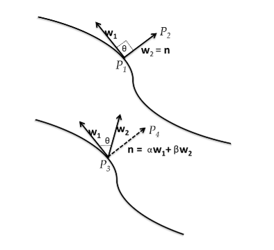
Figure 1: Orientation of CLVs on a most attracting material line (upper line) and on a neighbouring material line (lower line). The distance $\lVert P_{2}-P_{1}\rVert$ decreases faster than $\lVert P_{4}-P_{3}\rVert$ since in the second curve the normal vector connecting the points $P_{3}$ and $P_{4}$ is expressed as a linear combination of both the CLVs.

Along this curve, for any point $P_{1}$ we can chose a point $P_{2}$ which is on the normal vector to the curve in $P_{1}$, ${\bf n}$. Because of (11), the distance between these two points decreases as

$$\lVert P_{2}-P_{1}\rVert\propto\lVert{\bf w}_{2}\rVert\approx e^{\lambda_{2}(t^{\prime}-t)}.$$ (24)

Consider now a point $P_{3}$ on a nearby curve, and a point $P_{4}$ laying on the normal vector to the curve in $P_{3}$. The normal vector ${\bf n}$ at $P_{3}$ can be written as a linear combination of ${\bf w}_{1}$ and ${\bf w}_{2}$ and, considering again (11), one has thus

$$\lVert P_{4}-P_{3}\rVert=\lVert\alpha{\bf w}_{1}+\beta{\bf w}_{2}\rVert\approx e^{\lambda_{1}(t^{\prime}-t)}>e^{\lambda_{2}(t^{\prime}-t)}.$$ (25)

The previous computation can be repeated analogously for ${\bf w}_{2}$. The same reasoning holds for ${\bf w}_{2}$.

It must be remarked that (22b) gives asymptotic information, but is defined for a particular instant of time. For every time instant the lines (22), together with the orthogonality condition $\theta(t)=\pi/2$, describe the so called tensorlines, and can be seen as the asymptotic version of shearless barriers Farazmand et al. (2014).

Taking into account these properties of the CLVs, we propose a definition to describe these asymptotic coherent patterns:

Definition II.1 (Hyperbolic Covariant Coherent Structures (HCCSs)).

At each time $t$, a Hyperbolic Covariant Coherent Structure, is an isoline of the hyperbolicity scalar field $\theta$ at the level $\theta=\pi/2$. Its attractive or repelling nature is determined by the CLVs aligned with it.

It is important to emphasize the difference between the information provided by FTLEs and the one provided by CLVs. FTLEs are the finite time version of Lyapunov’s exponents and, as shown in the appendix, are calculated as a mean time of the logarithms of the separation of two trajectories that start from near points. The FTLEs therefore give an average information over the time interval considered. Moreover, if the time interval is long enough, and the analyzed region can be considered ergodic, the dependence on initial conditions is lost and therefore the possibility of displaying possible structures. CLVs, on the contrary, as well as LVs, depend on a time instant and do not converge to the same value. CLVs therefore allow the definition of instant structures, which, however, give asymptotic information.

This approach presents some numerical challenges, CLVs are not fast to be computed as the FTLEs, and numerically, in order to identify the isolines, it is necessary to consider an interval of values for the angle. The HCCSs are thus computed here considering isoregion of $\theta\in[\frac{\pi}{2}-\delta,\,\,\frac{\pi}{2}]$, where $\delta$ is $0.087$ rads.

III Numerical Examples

The algorithm used in this work is the same presented in Ref. Ginelli et al. (2007), so only a schematic of its structure will be presented here. This algorithm can compute a large number of CLVs converging exponentially fast when invertible dynamics is considered. The basic idea is that, if the backward Lyapunov vectors basis $\{{\bf l}^{-}_{1}(t),\,\,{\bf l}^{-}_{2}(t)\}$ is evolved by means the the operator ${\bf F}$, it is always possible to keep it orthonormalized with a $QR$ decomposition and store the corresponding upper triangular projection matrix. It is then possible to exploit the informations contained in these upper triangular matrices to evolve backward in time arbitrary vectors that will converge to the CLVs Ginelli et al. (2007). This is done in five different phases, which are described in Appendix A.

In the next we investigate the hyperbolicity field $\theta$ for three different examples, which include one autonomous Hamiltonian flow and two non-autonomous two dimensional flows. The HCCSs emerging from the angle between the CLVs are compared with the FTLEs field, while their attractive or repelling nature will be discussed in terms of the CLVs. The algorithm for the search of the CLVs and the computation of the FTLEs explore the same dynamics, because it is used the same time interval. However, the final CLVs are found just for a temporal subinterval of the whole time used, see Appendix A and Appendix B.

Technical details about the three different examples are included in the Appendix B for a clearer description of the physical results in the following.

III.1 A simple autonomous Hamiltonian system

In this preliminary example we investigate the HCCSs in an autonomous Hamiltonian flow map. The time-independent Hamiltonian, corresponding to the streamfunction of the flow, is

$$H=\frac{x^{2}y}{2},$$ (26)

so that the dynamical equations of motion are

$$\frac{dx}{dt} = -\frac{x^{2}}{2},$$ (27a)

$$\frac{dy}{dt} = xy,$$ (27b)

with $x(t_{0})=x_{0}$, and $y(t_{0})=y_{0}$. Integration of Eq. (27) yields the trajectories of the system, shown in Figure 2a, with flow map

$$\bm{\phi}_{t_{0}}^{t}(x_{0},y_{0})=\begin{bmatrix}x(t)=-\frac{2x_{0}}{2+x_{0}t}\\ y(t)=y_{0}\left(1+\frac{x_{0}t}{2}\right)^{2}\end{bmatrix}.$$ (28)

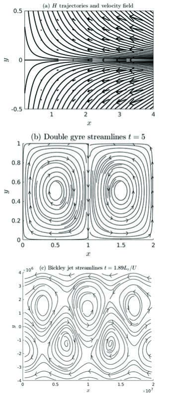
Figure 2: Panel (a): trajectories of the Hamiltonian system (28) (solid line). The trajectory $y=0$ represents a repulsive barrier for the system. Notice that the arrows indicate the flow velocity field, which is expressed on the right hand side of (27), and not the CLVs that are shown separately. Panels (b) and (c): streamlines for the double gyre and the Bickley jet, respectively.

Only the positive $x>0$ axis is considered, as the solution on the negative part blows up in finite time. As Figure 2a shows, the $y=0$ axis clearly divides the dynamics of the system into two different regions. There is no flux across this line, and the positive and negative $y$ regions are completely separated at each time. Furthermore, $y=0$ is the only material repelling line. Notice that in the Figure, the arrows do not indicate the CLVs but are just indicators of the magnitude of the flow. The trajectory $y=0$ behaves thus exactly as a material barrier dividing the system in two different regions, remains coherent at all time, and repels every close trajectories. We apply the CLVs theory to see if the angle between that vectors is able to detect such kind of structure.

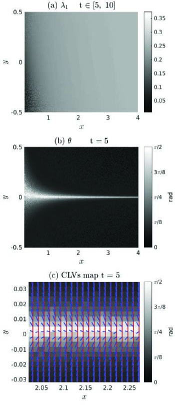
Figure 3: FTLEs and CLVs fields for the Hamiltonian system (27). (a) Maximum FTLEs field computed from (40); (b) $\theta$ field; (c) zoom of the domain to show the CLVs fields. Arrows are not used due to the arbitrariness of the orientation of the CLVs. The red lines are associated to ${\bf w}_{1}$, the expansion direction, while the blue lines are associated to with ${\bf w}_{2}$, the contraction direction.

Figure 3a shows the maximum FTLEs field computed in the time interval $t=[5,\,\,10]$ using definition (40). This field, referred to the initial grid conditions, does not highlight the $y=0$ barrier. Notice that if a bigger domain in the $y$ direction would have been selected, the FTLEs field would have showed a large scale modulation with larger values aligned along $y=0$. Figure 3b, shows the distribution of the CLVs angles at $t=5$. It is important to stress the fact that the FTLEs depend on a finite time interval while CLVs, and then $\theta$, on a particular instant of the time. The hyperbolicity field clearly shows values close to $\pi/2$ along the $y=0$ axis. The direction of the first (red) and second (blue) CLV is shown for an enlargement of a region close to this structure in Figure 3c. It is visible that the second CLV, that characterize the contraction direction, aside for numerical fluctuations, are aligned with the $\theta=\pi/2$ structure, indicating a contraction direction and thus a repelling structure, i.e. a barrier, forward in time. Notice also that near $x=0$, the velocity field is close to zero, so that the barrier there is not well defined. This suggests that the dynamics near the origin evolves with a different time scale.

Along the $x$ axis, $\theta=\pi/2$ remains constant for all the time. Consider in fact the propagator (7)

$${\bf F}(t,t^{\prime})=\begin{bmatrix}1/B^{2}&0\\ Bt^{\prime}y_{0}&B^{2}\end{bmatrix},$$ (29)

where

$$B=1+t^{\prime}x_{0}/2.$$ (30)

Along $y=0$, both the tangent linear propagator

$${\bf F}(t,t^{\prime})=\begin{bmatrix}1/B^{2}&0\\ 0&B^{2}\end{bmatrix}.$$ (31)

and the CGT (41)

$$\begin{split}{\bf C}(t,t^{\prime})&=\begin{bmatrix}1/B^{4}&0\\ 0&B^{4}\end{bmatrix},\quad y_{0}=0,\end{split}$$ (32)

are diagonal. If at time $t$ one has $\theta(t)=\pi/2$ for $y=0$, then

$${\bf w}_{1}(t)=\bm{\xi}_{1}=\begin{bmatrix}0\\ 1\end{bmatrix}\,\,\text{and}\,\,\,\,{\bf w}_{2}(t)=\bm{\xi}_{2}=\begin{bmatrix}1\\ 0\end{bmatrix},$$ (33)

where $\bm{\xi}_{1}$ and $\bm{\xi}_{2}$ are the eigenvectors of the CGT, and at time $t^{\prime}>t$

$$\begin{split}\cos(\theta(t^{\prime}))&\propto{\bf F}(t,t^{\prime}){\bf w}_{1}(t)\cdot{\bf F}(t,t^{\prime}){\bf w}_{2}(t)\\ &={\bf w}_{1}(t)\cdot{\bf C}(t,t^{\prime}){\bf w}_{2}(t)\\ &=0.\end{split}$$ (34)

This shows that $y=0$ is a repelling HCCSs.

III.2 Double gyre

The previous analysis is now applied to a time dependent system called double gyre flow Shadden et al. (2005); Onu et al. (2015), which is a simplification of observed geophysical flows consisting of two counter rotating vortices that expand and contract periodically. The tracers moving in this flow satisfy the following dynamical equations

$$\frac{dx}{dt}=-\pi A\sin(\pi f(x,t))\cos(\pi y),$$ (35a)

$$\frac{dy}{dt}=\pi A\cos(\pi f(x,t))\sin(\pi y)\frac{df(x,t)}{dx},$$ (35b)

$$f(x,t)=\epsilon\sin(\omega t)x^{2}+(1-2\epsilon\sin(\omega t))x,$$ (35c)

with initial condition $x(0)=x_{0}$, $y(0)=y_{0}$. The streamline of the flow at $t=5$ are shown in Figure 2b.

We consider two numerical experiments, DV1 and DV2, in which the CLVs are computed in two different time intervals with a non-null intersection. During DV1 we compute the CLVs in the interval $t=[5,\,\,10]$ and during DV2 for $t=[10,\,\,20]$. This is important, as will be shown in this section, to highlight that $\theta$ is a quantity that depends on a particular time instant and not on the time interval considered for its computation, as long as the interval considered is sufficiently long. Figure 4 shows a comparison between the angle $\theta$ and the FTLEs for this system. The first column is relative to DV1, while the second column is relative to DV2.

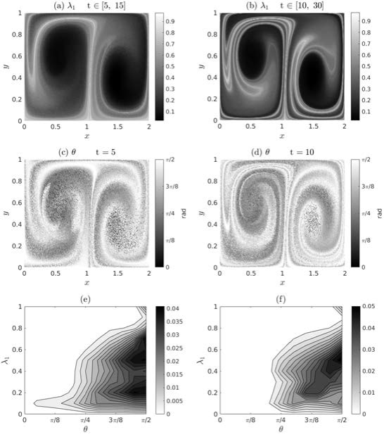
Figure 4: FTLEs, CLVs and joint probability plot for the experiments DV1 (left panels) and DV2 (right panels) of the double gyre system. The first column is referred to the experiment DV1 and the second column to DV2. Panels (a) and (b) show the maximum FTLE fields computed from (40). Panels (c) and (d) show the angle between the CLVs for the two experiments. Panels (e) and (f) show the joint probability between FTLEs and angles shown in the previous panels.

The $\lambda_{1}$ fields, the maximum FTLEs, are shown in Figures 4a and 4b for DV1 and DV2 respectively. The regions characterized by white color correspond to maximum exponential growth rate. Ridges of these regions correspond to the LCSs of the system according to the definition by Shadden et al Shadden et al. (2005). It is interesting to notice how, although in Figure 4b the ridges of the FTLEs are more developed, the $\lambda_{1}$ field converges to the same structures, and the maximum values do not change. The FTLEs give an overall information of the stretching and folding over the whole time interval considered, they can not say anything about the state of the coherent structures at a particular instant of time. Figures 4c and 4d show the hyperbolicity field $\theta$ computed for a particular time instant. The white colour here represents the maximum values of the hyperbolicity of the system, which means $\theta=\pi/2$, and highlight possible HCCSs as defined in II.1. Although the FTLEs and $\theta$ fields exhibit similar structures it is interesting to point out that the ridges of the FTLEs do not necessarily correspond to the regions of maximum hyperbolicity. Near the central regions of the two vortices, the hyperbolicity field has a noisy appearance, due the fact already discussed that in there the expansion and contraction directions are not well defined, and the CLVs become tangent to each other. Notice that this effect does not influence the detection of hyperbolic regions. Figures 4e and 4f highlight the differences between FTLEs and the $\theta$ fields shown respectively for the two experiments DV1 and DV2. As already mentioned, high values of the FTLEs do not necessarily correspond to high values of the $\theta$ field. The joint probability plots underline the fact that in general there is not a one to one relation between the $\theta$ and FTLE fields. In particular, small values of FTLEs are related to the broadest range of possible values for the angle between CLVs. This can be understood considering that the FTLEs measure the exponential growth rate of divergence of nearby trajectories. Where the FTLEs are smaller, the expansion and contraction directions are not well defined and a broader range for the possible values of the angle is obtained. Although there is not a clear relation between the two quantities it is interesting to point out that, for this example, the maximum values of FTLEs correspond to a reduced range of possible values of $\theta$, and for the DV2 experiment there is a univocal correspondence. The joint probabilities are asymmetric and their peaks towards the highest values of $\theta$ highlight the fact that the system is hyperbolic. In this case, in fact, it is possible to find, almost for every point of the domain, well defined expansion and contraction directions. It is interesting to note that the joint probability of Figure 4f is less asymmetric with respect to the correspondent joint probability in Figures 4e.

Figure 5 compares the HCCSs at time $t=10$ for the experiment DV2, found with the definition II.1, and the FTLEs field shown in Figure 4b. In the right panel there is a blow up of a region containing HCCSs. These pictures show that the instant structures highlighted by the HCCSs do not always correspond to the ridges of the FTLEs. The contours of the regions characterized by $\theta=\pi/2$ define the shapes of HCCSs, but to understand their attractive or repelling nature it is necessary looking at the CLVs that characterized those regions. The right panel of Figure 5 shows the repelling nature of the HCCSs in the zoomed region, since the contour is aligned with the second CLVs, ${\bf w}_{2}$, that define the contraction direction. Every particle of the tracer near these HCCSs will tend asymptotically to get away from them.

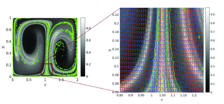
Figure 5: Comparison between the HCCSs at time $t=5$, green lines, computed for the experiment DV2 and the FTLEs field shown in Figure 4b. In the right panel there is a zoom of a portion of the domain in which are also shown the CLVs characterizing that region. Blue direction is contracting while red is expanding. Since the contour in this region is aligned with the second CLVs, the blue one, the character of the HCCSs here is repulsive.

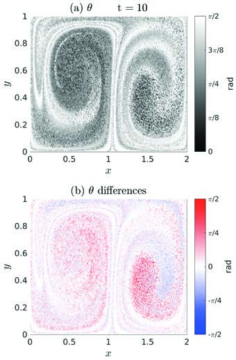
Figure 6: Comparison of the angle between CLVs, $\theta$, computed for the two experiments DV1 and DV2 at the same time $t=10$. Panel (a) show the evolution of the angle obtained in DV1 at $t=10$. Panel (b) shows the difference between the angle computed at the beginning of the experiment DV2 and the one computed at the end of the interval of the CLVs computation for the experiment DV1.

Figure 6 compares the evolution of $\theta$ field in DV1, computed at $t=10$, with the angles computed at the same time for the experiment DV2. The region of maximum hyperbolicity that appears in Figure 6a, corresponds to the same region that is found in Figure 4d. The difference between the two fields (Figure 6b) shows large values in regions with low hyperbolicity, and values close to zero for $\theta=\pi/2$ implying a convergence of the $\theta$ field. It should also be noted that the structure highlighted by the maximum hyperbolicity in the left part of the domain is pretty similar to the shown in Figure 4a. Once again, this underline that the FTLEs field gives an overall information and not an instantaneous one. The HLCSs found by using the FTLEs are, by definition, strongly related to the time interval chosen for the study, while the HCCSs, which correspond to instantaneous structures of maximum hyperbolicity, are independent of the time interval considered for their computation, as shown in these two experiments. The short-term behavior of passive tracer analyzed by HLCSs is strongly influenced by the time window used with respect to long-term behavior highlighted by HCCSs. It should also be noted that the HLCSs, once they have been found, are advected with the flow so as to ensure that they act as barriers for the passive tracer. However, this precludes the study of any new barriers that may arise in the flow in a time subinterval. These constraints are not present in the long-term study performed with HCCSs.

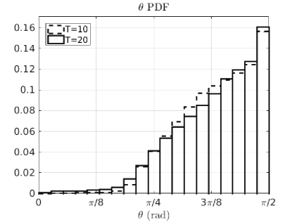
Figure 7: PDF of $\theta$ for the DV2 experiment computed at $t=10$ (dashed line) and at $t=20$ (full line).

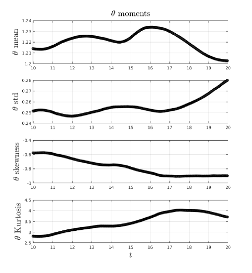
Figure 8: Evolution of the first four moments of the PDF for $\theta$ for the DV2 experiments in the interval $T2=[10\,\,20]$.

It is also interesting to consider the evolution of the PDF of the hyperbolicity field, $P(\theta,t)$. If the distribution is peaked around $\pi/2$, the expansion and contraction directions are almost everywhere perpendicular between each other. If the distribution is peaked around zero, the expansion and contraction directions are almost tangent everywhere. If the distribution is flat there is not a clear correlation between the expansion and contraction directions. Figures 7 shows the PDF of $\theta$ computed for the initial and final time of CLVs computation for the experiment DV2. The final PDF (full line) highlight an increasing of points with hight hyperbolicity, and an increment of points in the tail of the distribution near zero, with respect to the PDF computed at the beginning of the interval (dashed line). During the evolution in the interval $t=[10,\,\,20]$ the distribution becomes more asymmetric. The change in shape is visible also looking at the first four moments of the PDF computed at every time step in this time interval (Figure 8). All the moments of the distribution display only small changes in time during the evolution. This time interval is characterized by a mean value of $\theta$ oscillating in the range $[1.20,\,\,1.23]$. A monotonic change in the mean, possibly given by mixing, is visible after $t\approx 16$. It should be noted however that the range of this change is very small. The s.t.d. of the angles distributions is characterized by values that change within the interval $[0.25,\,\,0.28]$. After $t\approx 16$ the s.t.d. shows a monotonic increase, as a signature that, if the change in time is given by mixing, this must be of adiabatic nature and thus not resulting in a homogeneization of the field. The third moment of the PDF decreases in time from $-0.57$ to $-0.91$, showing thus a negatively skewed distribution. Finally, the kurtosis initially increases from $2.81$ to $4.03$, and then shows a slight decrease in values, generally indicating a less flat distribution than the normal distribution. Although the motion of the velocity field is periodic, the motion of the tracers in this flow is chaotic. This is the reason why we do not see in this interval a periodicity in the moments of the PDF for the variable $\theta$.

III.3 Bickley jet

The Bickley jet is an idealized model of a jet perturbed by a Rossby wave del Castillo-Negrete and Morrison (1993); Beron-Vera et al. (2010); Onu et al. (2015). The velocity field is given in terms of the stream function, $\psi(x,y,t)$, that can be decomposed as the sum of a mean flow $\psi_{0}(x,y,t)$ and a perturbation $\psi_{1}(x,y,t)$

$$\psi(x,y,t)=\psi_{0}(x,y)+\psi_{1}(x,y,t),$$ (36)

where

$$\psi_{0}(x,y)=c_{3}y-UL_{y}\tanh\left(\frac{y}{L_{y}}\right)+\\ \epsilon_{3}UL_{y}\text{sech}^{2}\left(\frac{y}{L_{y}}\right)\cos(k_{3}x),$$ (37)

and

$$\psi_{1}(x,y,t)=UL_{y}\text{sech}^{2}\left(\frac{y}{L_{y}}\right)\mathcal{R}e\left[\sum_{n=1}^{2}\epsilon_{n}f_{n}(t)e^{ik_{n}x}\right].$$ (38)

Following the work by Onu et al. Onu et al. (2015), the forcing is chosen as a solution that runs on the chaotic attractor of the Duffing Oscillator

$$\frac{d\varphi_{1}}{dt}=\varphi_{2}$$ (39a)

$$\frac{d\varphi_{2}}{dt}=-0.1\varphi_{2}-\varphi_{1}^{3}+11\cos(t),$$ (39b)

$$f_{1}(t)=f_{2}(t)=2.625\,10^{-2}\varphi_{1}(t/6.238\times 10^{5}).$$ (39c)

From now on the time will be scaled with the quantity $L_{x}/U$. The streamline of the flow at $t=1.89$ are shown in Figure 2c.

As for the double gyre, we show two experiments, $BJ1$ and $BJ2$, for which the end of the CLVs computation in the first experiment correspond with the first CLVs computation for the second experiment.

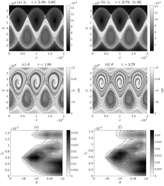
Figure 9: As in Figure 4, but for the two experiments BJ1 and BJ2.

The first column of Figure 9 shows the analysis for BJ1 and the second column for BJ2. Figures 9a and 9b, show the field of the maximum FTLEs, $\lambda_{1}$. Results show the convergence for the FTLE fields. Maximum values of $\lambda_{1}$ are reached in the central jet and around the boundaries of the vortices. Figures 9c and 9d show the angle between CLVs, where the white color indicates $\theta=\pi/2$. The $\theta$ fields clearly provide more details of the flow patterns than the FTLE fields. In agreement with the FTLE fields, values of $\theta$ close to $\pi/2$ are present in narrow bands in the central jet, in the center and around the vortices. The angle field shows however that not all the central band of the FTLEs field represents an HCCSs. The $\theta$ fields show also spiraling patterns within the vortices, which are instead not visible in the FTLE fields. The spiral patterns are particularly evident in the upper vortices, where the perturbation $\psi_{1}$ acts as a positive feedback to the flow. In the bottom vortices, the perturbation acts instead to weaken the flow. Figures 9e and 9f show the joint probability plots of the angles and the FTLEs just presented. These plots show that there is no clear relation between FTLEs and angle. For a given FTLE correspond many values of the angle between CLVs. As for the double gyre example, smaller values of the FTLEs correspond to the maximum range of possible values for $\theta$. However, differently from the double gyre, also high values of FTLEs correspond to a broad range of $\theta$ values. This can be explained considering that almost all the points corresponding to the highest values of FTLEs are contained in the central jet. In this region, the FTLEs converge to the same value, independently from the space position along the jet or time. Due to this convergence we do not have much information about smaller structures that can characterize the system in the jet region as instead shown by the $\theta$ field. For this reason, the joint probability plots do not exhibit a reduced range of $\theta$ values in correspondence of the highest FTLEs. The comparison between the BJ1 and BJ2 integrations shows that for the Bickley jet both the PDFs of the FTLEs and $\theta$ field are more stationary in time with respect the double gyre.

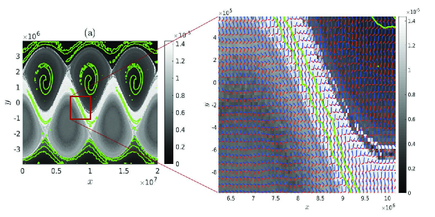
Figure 10: As in Figure 5, but for the two experiments BJ1 and BJ2.

The left panel of Figure 10 shows the superposition of HCCSs computed for $t=3.79$ for the experiment BJ2, green lines, and the FTLEs computed in the same experiments (Figure 9b). This figure remarks the fact that the central jet is not completely a HCCSs. HCCSs are also present at the border of the vortices and in the center part of the upper vortices. The right panel of Figure 10 show an enlargment into a portion of the central jet containing HCCSs and the CLVs in that part of the domain. In this picture it is possible to appreciate the repelling nature of the HCCSs looking the alignment of the contour with the second CLVs. It is interesting to point out that, looking at the FTLEs field, it is not possible to see ridges in the central jet. In this case it is not possible to find LCSs, if we use definition of LCSs based on the FTLEs field Shadden et al. (2005); Haller (2011), and this once again remark the difference between the HCCSs and LCSs.

Figure 11 shows the comparison between the angles at the end of the CLVs computation interval of the experiment $BJ1$ with the one computed at the beginning of the CLVs calculation interval for the $BJ2$ experiments. As for the double gyre, the comparison between Figure 11a and Figure 9d shows that regions characterized by $\theta=\pi/2$, i.e. the HCCSs, have the same structure. The difference between the two fields (Figure 11b), shows that these regions are characterized by smaller errors. In contrast, the regions with low hyperbolicity of Figure 11a appear to be more noisy with respect to the same regions computed for the $BJ2$ simulation (Figure 9d). In agreement with this, the difference between the two fields shows that the low hyperbolicity regions are characterized by larger errors (Figure 11b).

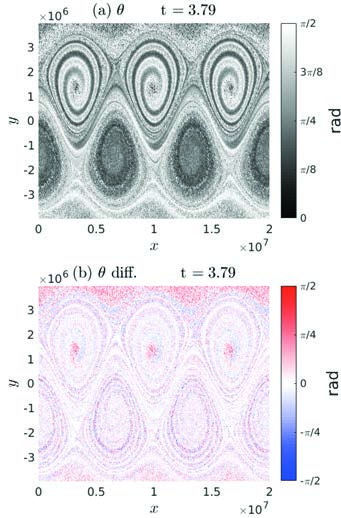
Figure 11: As in Figure 7, but for the BJ2 experiment.

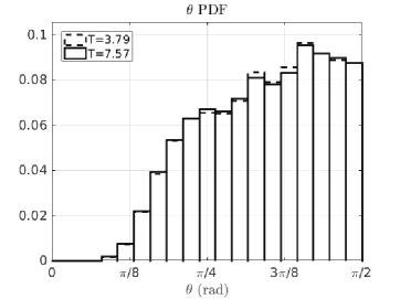
Figure 12: As in Figure 7, but for the BJ2 experiment.

Figure 12 shows the PDF of $\theta$ for the experiment BJ2 at the beginning and at the end of the CLVs computational interval. Results show that the PDF of the angle for this this interval remains stable. This is confirmed by the analysis of the moments of the distribution (not shown), which appear to be constant in time. With respect to the double gyre, the PDF for the Bickley jet is more flat indicating the presence of a larger number of points in which the CLVs are not orthogonal.

IV Conclusions

We have here proposed a new definition and a new computational framework to determine hyperbolic structures in a two dimensional flow based on Covariant Lyapunov Vectors. CLVs are covariant with the dynamics, invariant for temporal inversion and norm independent. These vectors are the natural mathematical entity to probe the asymptotic behaviour of the tangent space of a dynamical system. All these properties allow an exploration of the spatial structures of the flow, which can not be done using the Lyapunov Vectors bases due to their orthogonality.

CLVs are related to the contraction and expansion directions passing through a point of the tangent space, and the angle between them can be thus considered as a measure of the hyperbolicity of the system. This information can be summarized in a scalar field, the angle $\theta$, between the CLVs referred to the initial grid conditions, and used to define hyperbolic structures. The structures identified with the isolines of this field, characterized by $\theta=\pi/2$, are called Hyperbolic Covariant Coherent Structures. These patterns are the most repelling or attracting pointwise, in terms of the asymptotic behaviour of tracer particles, with respect to nearby structures at a given time. In terms of practical applications, this has important consequences, as it will provide an indicator for the long time transport of passive tracers such as for example oil spills in the ocean.

CLVs, and the correspondent $\theta$ field, have been computed for three numerical examples to compare how the behaviour of the particles tracer near HLCSs, highlighted by the FTLEs, can change asymptotically in time. The three examples include an Hamiltonian autonomous system, and two non-autonomous systems that are bounded or periodic. For all these examples it is possible to compute CLVs, HCCSs, and compare them with the HLCSs. Since the FTLEs tend to converge to LEs and lose their dependence on the initial conditions the angle between the CLVs could give more detailed information about possible structures that can emerge from the flow. This feature has been highlighted in particular for the Hamiltonian autonomous system, in which $\theta$ is able to detect the central barrier in contrast with the FTLEs field, and in the Bickley jet in which the FTLEs converge to the same value in the jet region and it is not possible to see any kind of particular finest structure. The use of $\theta$ provides information on the structures appearing at each time of the evolution of the flow, and the three examples underline that not always the HCCSs correspond to HLCSs and vice versa. So, particles tracer, such as chlorophyll or oil in water, can be maximally attracted or repelled by some HLCSs, but if we consider a different time interval and in particular the asymptotic behaviour of these particles, we can obtain a distribution that is completely different. Note that, in practice, the asymptotic time length can be considered as the time taken by two random initial basis to converge to the same BLVs basis.

It should be noticed that, while no fluxes can be present across the HLCSs the same does not necessary hold for all the structures appearing characterized by $\theta=\pi/2$. HCCSs can be found for every instant of time but they give the asymptotic information about the behaviour of the particles tracer near the HCCS at that instant of time and, for this reason, the zero flux requirement of the HLCSs is not necessary. HCCSs are not necessarily barrier, their meaning is different from the one of HLCSs.

For the three examples considered we have also computed HLCSs with the geodesic theory using the LCS tool Onu et al. (2015) (not shown). The results are in agreement with the discussion above. Looking at asymptotic time it is still possible to find particular structures emerging from flow, but clearly these structures not necessarily correspond to HLCSs computed for a particular time interval.

For the two non-autonomous systems we have considered the evolution of the PDFs of the $\theta$ field and the evolution of its first four moments. For the Bickley jet the probability distribution of the angle is stationary in time, and so its moments, but for the double gyre it is possible to appreciate a small variation in time for the PDF. The information deriving by the evolution of the $\theta$ field, related to the variation of the strength of the hyperbolicity field, could be used to characterize the dynamical mixing of the system.

Finally, future studies will have to address the detection of hyperbolic structures beyond analytical systems, i.e. for two-dimensional turbulent flows. This will be particularly interesting for flows at the transition between balance and lack of balance Badin et al. (2011); Badin (2014, 2013); Ragone and Badin (2016), where the detection of HCCSs can shed light both on the structure of mixing and on the forward cascade of energy to dissipation, or the lack of thereof. In particular, the evolution of the moments of the PDF of $\theta$ could be used to define an index of dynamical mixing for the system under study. Particularly interesting will be the behaviour of the HCCSs in presence of intermittency. We can conjecture that in particular cases, such as e.g. the merging of two vortices, the instantaneous structures underlined by the HCCS can give reliable information of the asymptotic tracer dynamics, that is the dynamics after the merging event. This is however left for future studies.

Appendix A Description of the algorithm

The algorithm for the identification of CLVs is based on five different phases:

1. Initialization (T1): this preliminary step is used to find the initial backward Lyapunov vector bases $\{{\bf l}^{-}_{1}(t),\,\,{\bf l}^{-}_{2}(t)\}$ for a whole set of initial conditions Benettin et al. (1980). A set of initial condition $\{{\bf x_{0}}\}\in D$ and two sets of initial orthonormal random bases are defined in the tangent spaces at every point at time $t_{0}$. The second set is necessary to check the convergence to the backward Lyapunov vectors bases. The initial conditions and the random bases are evolved respectively with (1) and (6) until the convergence of the two bases is reached with the desired accuracy. The convergence toward the Lyapunov vectors is typically exponential in time Ginelli et al. (2007); Goldhirsch et al. (1987). At every time step, for every initial condition, the evolved vectors are stored as column of a matrix that is decomposed with a QR decomposition. The last passage is implemented in order to find the new orthogonal basis at every time step, and the upper triangular matrix containing the coefficients that allow to express the old basis in terms of the new one.

2. Forward Transition (T2): the backward Lyapunov bases are evolved from time $t$ to $t^{\prime}$. The evolution is done with the help of (1), (6) and the $QR$ decomposition for every evolution step. We indicate with ${\bf X}(t_{k})$ the matrix which columns contain the new bases at time $t_{k}$, and with ${\bf R}(t_{k-1},\,t_{k})$ the correspondent upper triangular matrix. During this step both the local Lyapunov bases and upper triangular matrices are stored. The diagonal elements $({\bf R}(t_{k-1},\,t_{k}))_{ii}$ of the upper triangular matrices give information about the local growth rates of the bases vectors at a given time $t_{k}$, and they are used to compute the FTLEs as a time average

   $$\lambda_{i}=\frac{1}{t^{\prime}-t}\sum_{k=0}^{N-1}\log({\bf R}(t_{k-1},\,t_{k}))_{ii},$$ (40)

   where $N$ time step are considered between $t$ and $t^{\prime}$. If the LEs exist, (40) will converge to them for a sufficiently long evolution. It is worth to note that sometimes the FTLEs are computed using a different method, that is using the so called Cauchy Green Tensor (CGT) defined as

   $${\bf G}(t,t^{\prime})={\bf F}(t,t^{\prime})^{\top}{\bf F}(t,t^{\prime}).$$ (41)

   This operator is also known as deformation tensor, whose eigenvalues $\mu_{i}(t_{0},t)$, and eigenvectors $\bm{\xi}_{i}(t_{0},t)$, satisfy

   $${\bf G}(t,t^{\prime})\bm{\xi}_{i}(t,t^{\prime})=\mu_{i}(t,t^{\prime})\bm{\xi}_{i}(t,t^{\prime}),$$ (42a)

   $$\mu_{1}(t,t^{\prime})>\mu_{2}(t,t^{\prime})>0,$$ (42b)

   $$\bm{\xi}_{1}(t,t^{\prime})\,\bot\,\bm{\xi}_{2}(t,t^{\prime}).$$ (42c)

   From a geometric point of view, a set of initial conditions corresponding to the unit sphere is mapped by the dynamics into an ellipsoid, with principal axis aligned in the direction of the eigenvectors of the CGT and with length determined by the correspondent eigenvalues. The eigenvalues of the CGT determine the FTLEs as

   $$\lambda_{i}(t,t^{\prime})=\frac{1}{2(t^{\prime}-t)}\log(\mu_{i}(t,t^{\prime})),$$ (43)

   where the dependence on the starting position has here been suppressed. This second method for the computation of the FTLEs exhibits some problems, for example, if just one finite local growth rate is taken into account considering a large time interval, (43) teds to zero and not to the LEs. The first method should be preferred.

3. Forward Dynamics (T3): in this step the trajectories and the bases are further evolved from time $t^{\prime}$ to time $t^{\prime\prime}$ using (1) and (6). This time interval should grant the convergence, during the backward dynamic, to the CLVs. During this step only the upper triangular matrices are stored and are used to continue the computation of the FTLEs using (43).

4. Backward Transition (T4): in this step random upper triangular matrices are generated for every point of the grid, ${\bf C}$. These matrices contain the expansion coefficients of a set of two generic vectors (expressed as column of a matrix) in terms of the ${L^{-}}$ bases. Using the stored matrices ${\bf R}$ of the step 3, these matrices are evolved backward in time, until time $t^{\prime}$, using the following relation:

   $${\bf C}(t_{n})={\bf R}^{-1}(t_{n},t_{n+1}){\bf C}(t_{n+1}){\bf D}(t_{n},t_{n+1}),$$ (44)

   where $t_{n}$ and $t_{n+1}$ are time step between $t^{\prime}$ and $t^{\prime\prime}$. This method uses all the information contained in ${\bf R}$ and not just the diagonal part of the matrix. The ${\bf D}$ diagonal matrices contain the column norm of ${\bf C}$. Using Eq. (44) it is possible to show Ginelli et al. (2007) that the generic vectors chosen will be aligned with the CLVs. Note that when a trajectory passes close to tangency of an invariant manifold, the matrices $C$ can be ill-defined, and so a little amount of noise on the diagonal element of these matrices, or an average on the diagonal elements of the neighbor matrices is used to correct the problem.

5. Backward Dynamics (T5): in this final part of the algorithm, (44) is used with the ${\bf R}$ matrices of the step 2 to evolve backward the upper triangular matrices ${\bf C}$, from time $t^{\prime}$ to time $t$. In this phase the backward Lyapunov bases stored can be used to write the CLVs. The matrix containing in each columns the different CLVs at a given point in space and time, ${\bf W}$, can thus be written as

   $${\bf W}(t_{n})={\bf C}(t_{n}){\bf X}(t_{n}).$$ (45)

   For a two dimensional system, the algorithm could be optimized making use of (18). One can follow the first step (T1) of the previous algorithm to find the convergence toward the backward Lyapunov bases in the time interval $[t_{0},\,\,t]$. After this first step it is possible to carry on the evolution of the vectors, as in the second step (T2) during the time interval $[t,\,\,t^{\prime}]$, without saving the triangular matrices. In the same way it is possible to repeat the step (T1) but for a backward evolution during the time interval $[t^{\prime\prime},\,\,t^{\prime}]$ to find the forward Lyapunov bases and then continue the backward evolution as in the step (T2) during the time interval $[t^{\prime},\,\,t]$. At this stage it is possible to consider directly the first backward Lyapunov vectors and the second forward Lyapunov vectors in the time interval $[t,\,\,t^{\prime}]$ as the CLVs. In this algorithm there are just four steps and not five as in the one presented above, but for two times one has to consider the convergence step (T1) that is more time consuming in respect to the steps (T4) or (T5). It should be noted that in this algorithm, the forward and the backward evolutions could be done in parallel. The comparison between this algorithm and the one used for this study is left for future studies.

Appendix B Technical details of the numerical examples

B.1 Hamiltonian system

For the simple Hamiltonian flow we consider the domain $x=[0.2,\,\,4]$, $y=[-0.5,\,\,0.5]$, a resolution of $300\times 300$ grid points and a time step $dt=0.01$. The CLVs are computed just for $t=5$, so the phase T2 and T5 includes just a few time steps. The forward and backward evolution is done in the time interval $T=[5,\,\,10]$. From $t=0$ to $t=5$ the algorithm passes through the initialization phase (see Appendix A) to find the backward Lyapunov vectors bases. In Figure 13 it is shown the convergence for the spatial average of the scalar product between the starting random bases chosen.

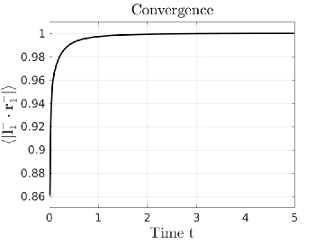
Figure 13: Convergence of the averaged scalar product for the two random bases chosen for the initialization of the numerical algorithm for the Hamiltonian system (27).

B.2 Double gyre

The parameters used for the double gyre example are $A=0.1$, $\epsilon=0.1$ and $\omega=\pi/5$. The spatial domain is $x=[0,\,\,2]$, $y=[0,\,\,1]$, with spatial resolution of $400\times 200$ points and time step $dt=0.02$. Two experiments, DV1 and DV2, involving different CLVs computational time interval are considered and summarized in Tab. 1.

	T1	T2	T3	T4	T5
DV1	$0\to 5$	$5\to 10$	$10\to 15$	$10\leftarrow 15$	$5\leftarrow 10$
DV2	$0\to 10$	$10\to 20$	$20\to 30$	$20\leftarrow 30$	$10\leftarrow 20$

Table 1: The five temporal windows of the numerical algorithm used for the two experiments DV1 and DV2.

During the initial phase of the numerical algorithm for the calculation of the CLVs, the average of the scalar product of the two initial random bases does not converge exactly to one (not shown here). This is because near the central regions of the two vortices of the double gyre, the expansion and contraction directions are not well defined, the CLVs become tangent to each other, and their separation is difficult to attain.

B.3 Bickley jet

The parameters used for this example are $U=62.66$, $c_{2}=0.205U$, $c_{3}=0.461U$, $L_{y}=1.77\times 10^{6}$, $\epsilon_{2}=0.04$, $\epsilon_{3}=0.3$, $L_{x}=6.371\pi\times 10^{6}$, $k_{n}=2\pi n/L_{x}$. The spatial domain considered is $x=[0,\,\,L_{x}]$, $y=[-2.25,\,\,2.25]L_{y}$, with a resolution of $500\times 250$ grid points and a time step of $dt=1800$. Two different time windows evolutions are considered, experiments $BJ1$ and $BJ2$, and summarized in Tab. 2.

	T1	T2	T3	T4	T5
BJ1	$0\to 1.89$	$1.89\to 3.79$	$3.79\to 5.68$	$3.79\leftarrow 5.68$	$1.89\leftarrow 3.79$
BJ2	$0\to 3.79$	$3.79\to 7.57$	$7.57\to 11.36$	$7.57\leftarrow 11.36$	$3.79\leftarrow 7.57$

Table 2: The five temporal windows of the algorithm used for the two experiments BJ1 and BJ2. Times have been rescaled with $L_{x}/U$.

References

- Dombre et al. (1986) Dombre, T.; Frisch, U.; Greene, J.M.; Hénon, M.; Mehr, A.; Soward, A.M. Chaotic streamlines in the ABC flows. J. Fluid Mech. 1986, 167, 353–391.
- Haller (2015) Haller, G. Lagrangian coherent structures. Annu. Rev. Fluid Mech. 2015, 47, 137–162.
- Kelley et al. (2013) Kelley, D.H.; Allshouse, M.R.; Ouellette, N.T. Lagrangian coherent structures separate dynamically distinct regions in fluid flows. Phys. Rev. E 2013, 88, 013017.
- Chian et al. (2014) Chian, A.C.L.; Rempel, E.L.; Aulanier, G.; Schmieder, B.; Shadden, S.C.; Welsch, B.T.; Yeates, A.R. Detection of coherent structures in photospheric turbulent flows. Astrophys. J. 2014, 786, 51.
- Pierrehumbert and Yang (1993) Pierrehumbert, R.T.; Yang, H. Global chaotic mixing on isentropic surfaces. J. Atmos. Sci. 1993, 50, 2462–2480.
- Doerner et al. (1999) Doerner, R.; Hübinger, B.; Martienssen, W.; Grossmann, S.; Thomae, S. Stable manifolds and predictability of dynamical systems. Chaos Solitons Fractals 1999, 10, 1759–1782.
- Haller and Yuan (2000) Haller, G.; Yuan, G. Lagrangian coherent structures and mixing in two-dimensional turbulence. Phys. D 2000, 147, 352 – 370.
- Haller (2001) Haller, G. Distinguished material surfaces and coherent structures in three-dimensional fluid flows. Phys. D 2001, 149, 248 – 277.
- Lapeyre (2002) Lapeyre, G. Characterization of finite-time Lyapunov exponents and vectors in two-dimensional turbulence. Chaos 2002, 12, 688–698.
- Shadden et al. (2005) Shadden, S.C.; Lekien, F.; Marsden, J.E. Definition and properties of Lagrangian coherent structures from finite-time Lyapunov exponents in two-dimensional aperiodic flows. Phys. D 2005, 212, 271 – 304.
- Lekien et al. (2007) Lekien, F.; Shadden, S.C.; Marsden, J.E. Lagrangian coherent structures in n-dimensional systems. J. Math. Phys. 2007, 48.
- Sulman et al. (2013) Sulman, M.H.; Huntley, H.S.; Jr., B.L.; Jr., A.K. Leaving flatland: Diagnostics for Lagrangian coherent structures in three-dimensional flows. Phys. D 2013, 258, 77 – 92.
- Rypina et al. (2007) Rypina, I.I.; Brown, M.G.; Beron-Vera, F.J.; Koçak, H.; Olascoaga, M.J.; Udovydchenkov, I.A. On the Lagrangian dynamics of atmospheric zonal jets and the permeability of the stratospheric Polar Vortex. J. Atmos. Sci. 2007, 64, 3595–3610.
- Rypina et al. (2010) Rypina, I.I.; Pratt, L.J.; Pullen, J.; Levin, J.; Gordon, A.L. Chaotic Advection in an archipelago. J. Phys. Oceanogr. 2010, 40, 1988–2006.
- Beron-Vera et al. (2008) Beron-Vera, F.J.; Olascoaga, M.J.; Goni, G.J. Oceanic mesoscale eddies as revealed by Lagrangian coherent structures. Geophys. Res. Lett. 2008, 35.
- Waugh and Abraham (2008) Waugh, D.W.; Abraham, E.R. Stirring in the global surface ocean. Geophys. Res. Lett. 2008, 35. L20605.
- Bettencourt et al. (2012) Bettencourt, J.H.; López, C.; Hernández-García, E. Oceanic three-dimensional Lagrangian coherent structures: A study of a mesoscale eddy in the Benguela upwelling region. Ocean Model. 2012, 51, 73 – 83.
- Harrison and Glatzmaier (2012) Harrison, C.S.; Glatzmaier, G.A. Lagrangian coherent structures in the California Current System, sensitivities and limitations. Geophys. Astrophys. Fluid Dyn. 2012, 106, 22–44.
- Waugh et al. (2012) Waugh, D.W.; Keating, S.R.; Chen, M.L. Diagnosing ocean stirring: comparison of relative dispersion and finite-time Lyapunov exponents. J. Phys. Oceanogr. 2012, 42, 1173–1185.
- Mukiibi et al. (2016) Mukiibi, D.; Badin, G.; Serra, N. Three-dimensional chaotic advection by mixed layer baroclinic instabilities. J. Phys. Oceanogr. 2016, 46, 1509–1529.
- Joseph and Legras (2002) Joseph, B.; Legras, B. Relation between Kinematic Boundaries, Stirring, and Barriers for the Antarctic Polar Vortex. J. Atmos. Sci. 2002, 59, 1198–1212.
- d’Ovidio et al. (2004) d’Ovidio, F.; Fernández, V.; Hernández-García, E.; López, C. Mixing structures in the Mediterranean Sea from finite-size Lyapunov exponents. Geophys. Res. Lett. 2004, 31.
- Cencini and Vulpiani (2013) Cencini, M.; Vulpiani, A. Finite size Lyapunov exponent: review on applications. J. Phys. A 2013, 46, 254019.
- Karrasch and Haller (2013) Karrasch, D.; Haller, G. Do finite-size Lyapunov exponents detect coherent structures? Chaos 2013, 23.
- Karrasch (2015) Karrasch, D. Attracting Lagrangian coherent structures on Riemannian manifolds. Chaos 2015, 25.
- Mancho et al. (2013) Mancho, A.M.; Wiggins, S.; Curbelo, J.; Mendoza, C. Lagrangian descriptors: A method for revealing phase space structures of general time dependent dynamical systems. Communications in Nonlinear Science and Numerical Simulation 2013, 18, 3530 – 3557.
- Lopesino et al. (2017) Lopesino, C.; Balibrea-Iniesta, F.; García-Garrido, V.; Wiggins, S.; Mancho, A. A theoretical framework for Lagrangian descriptors. Int. J. Bifurcat. Chaos 2017, 27, 1730001.
- Vortmeyer-Kley et al. (2016) Vortmeyer-Kley, R. ; Gräwe, U. ;Feudel, U. Detecting and tracking eddies in oceanic flow fields: a Lagrangian descriptor based on the modulus of vorticity. Nonlin. Process. Geophys. 2016, 23, 159–173.
- Froyland et al. (2010) Froyland, G.; Lloyd, S.; Santitissadeekorn, N. Coherent sets for nonautonomous dynamical systems. Phys. D 2010, 239, 1527 – 1541.
- Thiffeault (2010) Thiffeault, J.L. Braids of entangled particle trajectories. Chaos 2010, 20, 017516.
- Mundel et al. (2014) Mundel, R.; Fredj, E.; Gildor, H.; Rom-Kedar, V. New Lagrangian diagnostics for characterizing fluid flow mixing. Phys. Fluids 2014, 26, 126602.
- Skokos et al. (2007) Skokos, C.; Bountis, T.; Antonopoulos, C. Geometrical properties of local dynamics in Hamiltonian systems: The Generalized Alignment Index (GALI) method. Phys. D 2007, 231, 30 – 54.
- Cincotta and Simo (2000) Cincotta, P.M.; Simo, C. Simple tools to study global dynamics in non-axisymmetric galactic potentials. Astron. Astrophys. Suppl. 2000, 147, 205 – 228.
- Szezech et al. (2013) Szezech, J.; Schelin, A.; Caldas, I.; Lopes, S.; Morrison, P.; Viana, R. Finite-time rotation number: A fast indicator for chaotic dynamical structures. Phys. Lett. A 2013, 377, 452 – 456.
- Szezech et al. (2012) Szezech, J.D.; Caldas, I.L.; Lopes, S.R.; Morrison, P.J.; Viana, R.L. Effective transport barriers in nontwist systems. Phys. Rev. E 2012, 86, 036206.
- Jr. et al. (2009) Jr., J.D.S.; Caldas, I.L.; Lopes, S.R.; Viana, R.L.; Morrison, P.J. Transport properties in nontwist area-preserving maps. Chaos 2009, 19, 043108.
- Haller (2011) Haller, G. A variational theory of hyperbolic Lagrangian Coherent Structures. Phys. D 2011, 240, 574 – 598.
- Farazmand and Haller (2012) Farazmand, M.; Haller, G. Erratum and addendum to A variational theory of hyperbolic Lagrangian coherent structures [Phys. D 240 (2011) 574-598]. Phys. D 2012, 241, 439–441.
- Karrasch (2012) Karrasch, D. Comment on A variational theory of hyperbolic Lagrangian coherent structures [Phys. D 240 (2011) 574-598]. Phys. D 2012, 241, 1470–1473.
- Farazmand and Haller (2012) Farazmand, M.; Haller, G. Computing Lagrangian coherent structures from their variational theory. Chaos 2012, 22.
- Farazmand and Haller (2013) Farazmand, M.; Haller, G. Attracting and repelling Lagrangian coherent structures from a single computation. Chaos 2013, 23.
- Blazevski and Haller (2014) Blazevski, D.; Haller, G. Hyperbolic and elliptic transport barriers in three-dimensional unsteady flows. Phys. D 2014, 273-274, 46 – 62.
- Haller and Beron-Vera (2012) Haller, G.; Beron-Vera, F.J. Geodesic theory of transport barriers in two-dimensional flows. Phys. D 2012, 241, 1680 – 1702.
- Farazmand et al. (2014) Farazmand, M.; Blazevski, D.; Haller, G. Shearless transport barriers in unsteady two-dimensional flows and maps. Phys. D 2014, 278-279, 44 – 57.
- Serra and Haller (2016) Serra, M.; Haller, G. Objective Eulerian coherent structures. Chaos 2016, 26, 053110.
- Serra and Haller (2017a) Serra, M.; Haller, G. Forecasting long-lived Lagrangian vortices from their objective Eulerian footprints. Journal of Fluid Mechanics 2017, 813, 436?457.
- Serra and Haller (2017b) Serra, M.; Haller, G. Efficient computation of null geodesics with applications to coherent vortex detection. Proceedings of the Royal Society of London A: Mathematical, Physical and Engineering Sciences 2017, 473.
- Oseledec (1968) Oseledec, V.I. A multiplicative ergodic theorem. Lyapunov characteristic numbers for dynamical systems. Trans. Moscow Math. Soc. 1968, 19, 197–231.
- Ruelle (1979) Ruelle, D. Ergodic theory of differentiable dynamical systems. Publ. Math. IHES 1979, 50, 27–58.
- Wolfe and Roger M. (2007) Wolfe, C.L.; Roger M., S. An efficient method for recovering Lyapunov vectors from singular vectors. Tellus A 2007, 59, 355–366.
- Ginelli et al. (2007) Ginelli, F.; Poggi, P.; Turchi, A.; Chaté, H.; Livi, R.; Politi, A. Characterizing dynamics with covariant Lyapunov vectors. Phys. Rev. Lett. 2007, 99, 130601.
- Fro (2013) Computing covariant Lyapunov vectors, Oseledets vectors, and dichotomy projectors: A comparative numerical study. Phys. D 2013, 247, 18 – 39.
- Bosetti and Posch (2010) Bosetti, H.; Posch, H.A. Covariant Lyapunov vectors for rigid disk systems. Chem. Phys. 2010, 375, 296 – 308.
- Xu and Paul (2016) Xu, M.; Paul, M.R. Covariant Lyapunov vectors of chaotic Rayleigh-Bénard convection. Phys. Rev. E 2016, 93, 062208.
- Wolfe and Samelson (2008) Wolfe, C.L.; Samelson, R.M. Singular vectors and time-dependent normal modes of a baroclinic wave-mean oscillation. J. Atmos. Sci. 2008, 65, 875–894.
- Schubert and Lucarini (2015) Schubert, S.; Lucarini, V. Covariant Lyapunov vectors of a quasi-geostrophic baroclinic model: analysis of instabilities and feedbacks. Q. J. R. Meteor. Soc. 2015, 141, 3040–3055.
- Schubert and Lucarini (2016) Schubert, S.; Lucarini, V. Dynamical analysis of blocking events: spatial and temporal fluctuations of covariant Lyapunov vectors. Q. J. R. Meteor. Soc. 2016, 142, 2143–2158.
- (58) Vannitsem, S.; Lucarini, V. Statistical and dynamical properties of covariant Lyapunov vectors in a coupled atmosphere-ocean model-multiscale effects, geometric degeneracy, and error dynamics. J. Phys. A, 49, 224001.
- Yang and Radons (2008) Yang, H.L.; Radons, G. When can one observe good hydrodynamic Lyapunov modes? Phys. Rev. Lett. 2008, 100, 024101.
- Yang and Radons (2010) Yang, H.L.; Radons, G. Comparison between covariant and orthogonal Lyapunov vectors. Phys. Rev. E 2010, 82, 046204.
- Kuptsov and Parlitz (2012) Kuptsov, P.V.; Parlitz, U. Theory and computation of covariant Lyapunov vectors. J. Nonlinear Sci. 2012, 22, 727–762.
- Sala et al. (2012) Sala, M.; Manchein, C.; Artuso, R. Estimating hyperbolicity of chaotic bidimensional maps. Int. J. Bifurcat. Chaos 2012, 22, 1250217.
- Ginelli et al. (2013) Ginelli, F.; Chate, H.; Livi, R.; Politi, A. Covariant Lyapunov vectors. J. Phys. A 2013, 46, 254005.
- d ’Ovidio et al. (2009) d’Ovidio, F.; Shuckburgh, E.; Legras, B. Local mixing events in the upper troposphere and lower stratosphere. Part I: Detection with the Lyapunov Diffusivity. J. Atmos. Sci. 2009, 66, 3678–3694.
- Eckmann and Ruelle (1985) Eckmann, J.P.; Ruelle, D. Ergodic theory of chaos and strange attractors. Rev. Mod. Phys. 1985, 57, 617–656.
- Onu et al. (2015) Onu, K.; Huhn, F.; Haller, G. LCS Tool: A computational platform for Lagrangian coherent structures. J. Comput. Sci. 2015, 7, 26 – 36.
- del Castillo-Negrete and Morrison (1993) del Castillo-Negrete, D.; Morrison, P.J. Chaotic transport by Rossby waves in shear flow. Phys. Fluids A 1993, 5, 948–965.
- Beron-Vera et al. (2010) Beron-Vera, F.J.; Olascoaga, M.J.; Brown, M.G.; Koçak, H.; Rypina, I.I. Invariant-tori-like Lagrangian coherent structures in geophysical flows. Chaos 2010, 20, 017514.
- Badin et al. (2011) Badin, G.; Tandon, A.; Mahadevan, A. Lateral mixing in the pycnocline by baroclinic mixed layer eddies. J. Phys. Oceanogr. 2011, 41, 2080–2101.
- Badin (2014) Badin, G. On the role of non-uniform stratification and short-wave instabilities in three-layer quasi-geostrophic turbulence. Phys. Fluids 2014, 26, 096603.
- Badin (2013) Badin, G. Surface semi-geostrophic dynamics in the ocean. Geophys. Astro. Fluid Dyn. 2013, 107, 526–540.
- Ragone and Badin (2016) Ragone, F.; Badin, G. A study of surface semi-geostrophic turbulence: freely decaying dynamics. J. Fluid Mech. 2016, 792, 740–774.
- Benettin et al. (1980) Benettin, G.; Galgani, L.; Giorgilli, A.; Strelcyn, J.M. Lyapunov Characteristic Exponents for smooth dynamical systems and for hamiltonian systems; A method for computing all of them. Part 2: Numerical application. Meccanica 1980, 15, 21–30.
- Goldhirsch et al. (1987) Goldhirsch, I.; Sulem, P.L.; Orszag, S.A. Stability and Lyapunov Stability of Dynamical Systems: A Differential Approach and a Numerical Method. Phys. D 1987, 27, 311–337.