Discovering Political Topics in Facebook Discussion threads with Graph Contextualization

Abstract

We propose a graph contextualization method, pairGraphText, to study political engagement on Facebook during the 2012 French presidential election. It is a spectral algorithm that contextualizes graph data with text data for online discussion thread. In particular, we examine the Facebook posts of the eight leading candidates and the comments beneath these posts. We find evidence of both (i) candidate-centered structure, where citizens primarily comment on the wall of one candidate and (ii) issue-centered structure (i.e. on political topics), where citizens’ attention and expression is primarily directed towards a specific set of issues (e.g. economics, immigration, etc). To identify issue-centered structure, we develop pairGraphText, to analyze a network with high-dimensional features on the interactions (i.e. text). This technique scales to hundreds of thousands of nodes and thousands of unique words. In the Facebook data, spectral clustering without the contextualizing text information finds a mixture of (i) candidate and (ii) issue clusters. The contextualized information with text data helps to separate these two structures. We conclude by showing that the novel methodology is consistent under a statistical model.

, , , , and

t1The authors gratefully acknowledge support from NSF grant DMS-1612456 and ARO grant W911NF-15-1-0423. t2The authors gratefully acknowledge support from Audencia Foundation Research grant.

1 Introduction

Social networking sites (SNSs) such as Facebook and Twitter now make up a major part of Internet communications (Ellison et al., (2007), Kaplan and Haenlein, (2010)), including political communication. By providing platforms for citizens to publicly communicate with each other and with politicians, SNSs may increase the accessibility of candidates and political dialog (Wellman et al.,, 2001) and motivate political engagement within the public (Williams and Gulati, (2013), Williams and Gulati, (2009), Hebshi and O’Gara, (2011), Kushin and Kitchener, (2009)). They also appear to facilitate the spread of false or offensive information, and a variety of forms of actors to reach micro-targeted publics with a high degree of efficiency (Kreiss and Mcgregor,, 2017). Since the 2008 US election particularly (Wattal et al.,, 2010), SNSs have been playing a significant role in advertising and interactions during the presidential elections.

Drawing meaning from the massive text corpora of political discussion threads on SNSs has been a major project of scholars working in text mining (Pang et al., (2008), Stieglitz and Dang-Xuan, (2013), Grimmer and Stewart, (2013)) and sentiment analysis in recent years. One popular text mining approach is the probabilistic topic models based on latent Dirichlet allocation (LDA) (Blei et al., (2003), Blei, (2012), Chang and Blei, (2009)), which have been extensively used in social science (Ramage et al.,, 2009). Sentiment analysis is another approach to analyze text. It focuses on understanding emotions in the text. Wang et al., (2012) provides a system for real-time sentiment analysis on Twitter during the 2012 US election. For instance, using sentiment analysis and regression, Stieglitz and Dang-Xuan, (2012) finds that political tweets on Twitter that contain stronger emotions receive more public interactions. There are also studies of how political sentiment on SNSs reflect the offline political landscape (Tumasjan et al.,, 2011), and how it can affect political elections (Choy et al.,, 2011).

Apart from the topic or sentiment information, patterns of political discussion on SNSs are also of great theoretical and empirical interests to scholars of communication and political science. Such platforms have long been heralded for their potential to foster a “public sphere” in which ordinary citizens can recognize one another and hear reasons both for and against their own points of view (Papacharissi, (2002)). More recent analyses of online political discourse are less optimistic, identifying instead vitriol, “trolling”, and larger patterns of partisan polarization. As a result, a great deal of research investigates the extent to which online actors are connected to political opponents (Adamic and Glance, (2005), Colleoni et al., (2014), Bakshy et al., (2015))

Another approach to understand structure of political discussions is social network analysis, which aims to identify influential political actors and communities in the discussions (Stieglitz and Dang-Xuan,, 2012) and to study properties of the communities (Robertson et al., (2010)) Gonzalez-Bailon et al., (2010)). One popular community detection approach is spectral clustering (Von Luxburg,, 2007), which is fast, easy to implement, and consistent in block models for network (Holland et al., (1983), Airoldi et al., (2008), Qin and Rohe, (2013)).

In this paper, we combine text mining and community detection to investigate the multiple dimensions of citizens’ interactions with political content coming from political actors. In our data, which come from the 2012 French election, citizens commented on presidential candidate’s Facebook posts. This creates a communication network between two types of units: (i) citizens and (ii) candidate-posts, as the eight presidential campaigns each has posts on Facebook, and citizens comment on the posts. This paper studies the structure of the resulting discussion threads.

The activities of the citizens are characterized by (i) which of the candidate-posts they comment on and (ii) the text of their comments. We are interested in two broad types of patterns in these activities: (i) candidate-centered structure, where citizens primarily comment on the wall of one candidate; and (ii) issue-centered structure, in which citizens’ attention and expression is directed towards a specific set of issues (e.g. economics, immigration, etc). To search for such patterns, we cluster the citizens based on their activities. In each cluster, we examine whether the activities of the citizens focus on particular candidates (i.e. candidate-centered)(Section 2.2) or whether the activities focus on certain political issues (i.e. issue-centered)(Section 4). This distinction reflects the possibility that the Facebook conversation might be organized more along lines of partisanship (candidate-centered), as opposed to matters of concern to “issue publics” (issue-centered) (Kim, (2009)).

There has been significant progress on both topic modeling for text (Blei,, 2012) and community detection for social networks (Airoldi et al., (2008)). Recently, there has been significant interest in clustering networks for which we have additional information on the citizens in networks (Chang and Blei, (2010); Binkiewicz et al., (2017)). In this paper, we extend these ideas to the setting of discussion threads. Our network is two-way or bi-partite, in which the two types of units, citizens and candidate-posts, are linked by commenting in a discussion thread. Below, we refer to the links showing which citizens commented on which candidate-posts as the network or the graph. We refer to both the text in candidate-posts and the text in citizen-comments as the text. The duality between citizens and candidate-posts also appears in the text; candidates say things differently from citizens.

A key difficulty in analyzing this process, and the key methodological innovation of this paper, is to combine these disparate sources of data, the graph information and the two types of text information (citizen-words and thread-words), in a meaningful way. We develop a graph contextualization technique, pairGraphText, to leverage high dimensional node covariates into spectral clustering. We extend and specialize the techniques of Binkiewicz et al., (2017) to deal with both (i) the asymmetrical nature of the network between citizens and candidate-posts, and (ii) the high dimensional and sparse nature of the text. With noticeable themes, four sub-populations and four sub-groups of the candidate-posts are uncovered by our method. We interpret the clusters by a word-content strategy: For each cluster, we (i) identify keywords, and then (ii) read through central conversations containing the keywords.

Our graph contextualization method, pairGraphText, is adaptable to symmetric or directed graphs, unipartite or bipartite, assortative or dis-assortative, weight or unweighted. It scales to hundreds of thousands of nodes and thousands of covariates (e.g. words). pairGraphText uses a sparsity penalty to select the key covariates that align with the graph. After combining the covariates with the graph, we use spectral clustering to compute a partition of the nodes. Finally, we provide diagnostics to identify key covariates to interpret the different clusters. Theorem 5.2 shows that our method is consistent under the Node-Contextualized Stochastic co-Blockmodel. Section 4 uses pairGraphText to identify the issue centered structure in the Facebook discussion threads. In Section 6, we compare pairGraphText to a state-of-the-art topic modeling method, relational topic model (RTM) (Chang and Blei,, 2009), by both the Facebook discussion threads and simulations. We show that RTM focuses more on the text data, while pairGraphText focuses more on the graph data.

This paper is organized as follows. In Section 2, we briefly describe the 2012 French presidential election, the discussion threads on Facebook, and the result of regularized spectral clustering without any contextualizing information. In Section 3, we introduce the graph contextualization technique, pairGraphText, which leverages node covariates in spectral clustering. In Section 4, we identify the issue-centered structure of the discussion threads using pairGraphText. The statistical consistency of our method is provided under the Node Contextualized Stochastic co-Blockmodel in Section 5. In Section 6, we discuss different choices for weights of words, and we compare pairGraphText with a state-of-the-art topic modeling method. Section 7 concludes with a discussion of our method.

2 Background and key summaries of the data

France’s presidential elections proceed in two stages. On April 22 2012, the first round of voting narrowed the field of candidates from ten to two; the second round, between François Hollande and Nicolas Sarkozy, took place on May 6. In these analyses, we focus on the eight candidates who received at least $1\%$ of the votes in the 1st round of the election. These eight candidates–François Hollande, Nicolas Sarkozy, Marine Le Pen, Jean-Luc Mélenchon, François Bayrou, Eva Joly, Nicolas Dupont-Aignan, and Philippe Poutou–made a total of 3239 posts on Facebook. In response, 92,226 Facebook users, which we call citizens, made 594,685 comments on the candidate-posts.

There are two main structures that we aim to detect and study in the conversation: (i) candidate-centered structure, where citizens primarily comment on the wall of one candidate; and (ii) issue-centered structure, in which citizens’ attention and expression is directed towards a specific set of issues (e.g. economics, immigration, etc).

2.1 The communication network

To study the structure of the conversations, we construct a weighted bi-partite network between citizens and candidate-posts (see Figure 1) from the discussion threads.

Figure 1: The Communication Network is a bi-partite graph between citizens and candidate-posts. Each edge weight corresponds to the number of times that a citizen comments on a candidate-post.

A citizen is linked to a candidate-post if and only if the citizen comments on the candidate-post. The weight of this link is the number of times the citizen comments on the candidate-post. To represent this network, we construct the weighted adjacency matrix $A\in\mathbb{R}^{92,226\times 3239}$ with

$$A_{ij}=\#\text{ of times of citizen $i$ comments on candidate-post $j$.}$$ (2.1)

Denote the degree of a citizen $i$, $d_{i}=\sum_{j}A_{ij}$, as the number of comments by citizen $i$. Denote the degree of a candidate-post $j$, $d_{j}=\sum_{i}A_{ij}$, as the number of comments underneath the candidate-post. Figure 2 shows the proportion of citizens who have at least $d$ comments, as a function of $d$. Figure 2 gives the same result for the post-degrees.

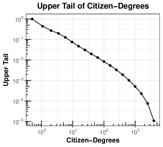
Figure 2: Upper Tail of Degrees. Figure (a) shows the upper tail of citizen-degrees. $90\%$ of the citizens write fewer than 10 comments, a small number of citizens write thousands of comments. Figure (b) shows the upper tail of post-degrees by candidate. The top three candidates: Hollande, Sarkozy, and Le Pen (on right), have the largest degrees.

2.2 Citizens’ attention-ratio towards candidates

Let $\zeta_{ij}$ be the number of times that citizen $i$ comments under candidate $j$’s wall. For each citizen $i$, we denote their attention-ratio as

$$\text{AttentionRatio}(i)=\frac{\max\limits_{\ell}\zeta_{i\ell}}{d_{i}}.$$

When the attention-ratio is one, it indicates the citizen only comment on one candidate-wall, while smaller attention-ratio indicates the citizen comments across different candidate-walls. We say that citizen $i$ focuses on candidate $j$ if $\zeta_{ij}\geq\zeta_{i\ell}$ for any candidate $\ell$. The citizens that have tied favorites are randomly assigned to one of their favorite candidates. Then, the citizens are naturally partitioned into eight clusters based on the candidates they focus on. Figure 3 shows the histogram of attention-ratio for all citizens with $d_{i}\geq 10$. Most of the mass of this histogram is close to one, indicating that most citizens primarily comment on one candidate-wall. This gives the first impression of candidate-centered structure.

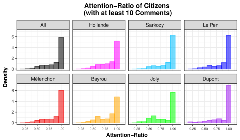
Figure 3: Distribution of Citizens’ Attention-Ratio. In this figure, we focus on citizens who have at least 10 comments. The first plot displays the histogram of attention-ratio for all citizens. The rest eight plots are for the eight citizen-clusters based on the candidates they focus on. We don’t display the citizens who focus on Poutou, because he attracts very few comments.

Categorizing the citizens based upon where they focus their attention produces a partition. For any partition of citizens, $\mathscr{P}:\{1,\dots,N_{C}\}\rightarrow\{1,\dots,K_{C}\}$ where $N_{C}=92,226$ is the number of citizens and $K_{C}$ is the number of citizen-clusters, define matrix $\Psi_{C}\in\mathbbm{R}^{K_{C}\times 8}$ such that for any $a\in\{1,\dots,K_{C}\}$ and $b\in\{1,\dots,8\}$,

$$[\Psi_{C}]_{a,b}=\frac{\text{$\#$ of comments from citizens in cluster $a$ under posts on $b$th candidate-wall}}{(\text{$\#$ of citizens in cluster $a$})\times(\text{$\#$ of posts on $b$th candidate-wall})}.$$ (2.2)

Figure 4 gives a balloon plot of $\Psi_{C}$ for the partition created by where citizens focus their attention. It also shows a clear candidate-centered structure: Each candidate has a corresponding citizen-cluster that mainly comment on their posts. Combined with the size of each citizen-cluster, it shows leading candidates attract larger clusters of citizens. See supplementary material for more evidence for candidate-centered structure.

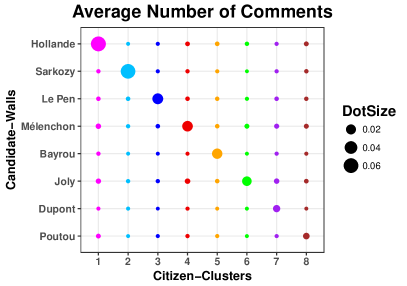
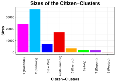
Figure 4: Citizen-Clusters Figure (a) shows interactions between the citizen-clusters and candidate-walls. The sizes of the balloons are the elements of $\Psi_{C}$ (defined in (2.2)). Figure (b) shows the number of citizens in each cluster. In Figure (b), we label each citizen-cluster by the corresponding candidate . For example, the first citizen-cluster is Hollande-centered from Figure (a), so we label it as 1 (Hollande) in Figure (b).

However, such strong candidate-centered structure, where citizens primarily comment on the wall of one candidate, does not lead to the conclusion that citizens devote their attention to candidates rather than issues. It might be an “illusion” from the “magnifying” effect of Facebook (Webster, (2014)). One possibility is many citizens may only follow one candidate on Facebook, so they can only see posts from one candidate. Even if they are interested in topics that are discussed by many candidates, they are likely to comment only on the candidate’s posts that they follow. In this case, even a slight more interest in one candidate can be magnified by Facebook to a strong candidate-centered structure. To understand whether the citizens’ attention is only directed by candidates, we dig more deeply into the discussion threads in the following sections.

Importantly, the partition of citizens in Figure 4, which is created by where citizens focus their attention, uses the additional information of which of the eight candidates writes each post. In other words, this partition of the rows of $A\in\mathbb{R}^{92,226\times 3239}$ uses a partition of the 3239 columns of $A$ which is defined by which candidate writes the post. The next sections will define two additional partitions of the citizens. Neither of these partitions will use the information of which candidate writes the post. The summary $\Psi_{C}$ will be computed with these new partitions to help interpret whether they are discovering candidate-centered structure.

2.3 Studying the graph using di-sim

Despite the overwhelming evidence for strong candidate-centered clusters in Figure 4, the spectral algorithm di-sim (Rohe et al., (2016)) finds a different partition of the citizens. Di-sim partitions both citizens and candidate-posts by applying a spectral clustering algorithm. It applies the singular value decomposition to a normalized version of the adjacency matrix $A$ (defined in (2.1)). By applying k-means to the top left and right singular vectors, di-sim partitions the citizens and posts to different clusters. Figure 5 displays the matrix $\Psi_{C}$ (defined in (2.2)) for the partition of citizens created by di-sim. Only the top three candidates have clusters that focus on them: Hollande and Sarkozy each has two clusters and Le Pen has one cluster that focuses on her. Other citizen-clusters (6,7,8) spread across multiple candidates.

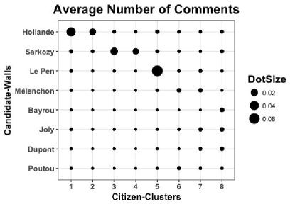
Figure 5: The Citizen-Clusters by DI-SIM. Similar to Figure 4, this figure shows the balloon plot of $\Psi_{C}$ corresponding to the citizen-clusters by di-sim.

One possible reason for the discrepancy between the attention-based partition and the partition from di-sim is that there may be some additional structure and di-sim is finding a mixture of the candidate-centered structure with that additional structure. pairGraphText, which we will introduce in the following sections, confirms that there is also an issue-centered structure in the network by incorporating text information.

3 Graph Contextualization with pairGraphText

As shown in Section 2, there are at least two good clusterings of the nodes (by attention-ratio or by di-sim). Given the potentially large number of plausible clusterings of the nodes, the overarching aim of graph contextualization is to find a co-clustering of $A$ (i.e. clustering both its rows and columns) such that these clusters align with a partition in the contextualizing information.

To quantify and utilize the contextualizing information, Section 3.1 describes how we preprocess the text in the discussion threads. Section 3.2 defines the document-term matrices to represent the text used by citizens and candidate-posts. Section 3.3 introduces the pairGraphText algorithm.

3.1 Preprocessing the text

To preprocess the text, we represent the text in document-terms, remove numbers, symbols (e.g. %, $@$, etc), and stop words (e.g. le, la, en, au, etc.) and transfer words into their roots by stemming. For example, maintenaient, maintenait, maintenant, maintenir are transferred into their root mainten.

3.2 Document-term matrices (node covariate matrices)

From the cleaned text, we retain two different sets of words: “citizen-words” which are contained by at least $0.1\%$ of the comments, and “thread-words” which are contained in at least $0.1\%$ of the contents in threads (i.e. posts and comments). In this data, over 99% of citizen-words and thread-words are overlapped, such as franc, vot, plus, etc. There are also thread-words that are not in citizen-words, such as confrontaient, relancait, etc.

To contextualize the citizens with the words that they write, define $X\in\mathbb{R}^{N_{C}\times M_{C}}$, where $N_{C}$ is the number of citizens and $M_{C}=2020$ is the number of citizen-words. For citizen $i$ and citizen-word $j$,

$$X_{ij}=\#\text{ of comments from citizen $i$ that contain citizen-word $j$}.$$

Representing the candidate-posts is not as simple. Candidate-posts provide platforms for conversations, but usually it is the comments underneath it that generate conversations. This phenomenon is colloquially referred to as “thread highjacking,” where the discussion thread (beneath a candidate-post) is used to discuss something other than what is discussed in the candidate-post. In particular, many of the candidate-posts direct their followers to interviews that happen in traditional media. Thus, to properly contextualize the thread, one must include the text that citizens are responding to, which is not necessarily the candidate-post. To represent the text that citizens are responding to when they post a comment in a thread, we use matrix $Y\in\mathbb{R}^{N_{P}\times M_{P}}$, where $N_{P}=3239$ is the number of candidate-posts and $M_{P}=2021$ is the number of thread-words. For candidate-post $i$ and thread-word $j$,

$$Y_{ij}= \bm{1}\{\text{candidate-post $i$ contains thread-word $j$}\}+$$

$$\#\text{ of comments underneath candidate-post $i$ that contain thread-word $j$}.$$

We refer to $X$ and $Y$ document-term matrices and consider them as node covariate matrices that contain the text information about both types of nodes (citizens and candidate-posts). The rows index the nodes (citizens or candidate-posts) and columns index the dictionaries (citizen-words or thread-words). Our setting allows citizen-covariates and post-covariates to differ in both type and number. In general, there could be various types of covariates. Note that categorical covariates should be re-expressed with dummy variables. In practice, node covariate matrices $X$ and $Y$ should be centered and scaled by column before analysis.

3.3 pairGraphText

pairGraphText is a refinement of Covariate Assisted Spectral Clustering (CASC) (Binkiewicz et al.,, 2017). In CASC, the graph is uni-partite. Denote $X\in\mathbb{R}^{N\times M}$ as the node covariate matrix and $L\in\mathbb{R}^{N\times N}$ as the regularized graph Laplacian

$$L=D_{C}^{-1/2}AD_{P}^{-1/2},$$ (3.1)

where $D_{C}$ and $D_{P}$ are diagonal matrices with $[D_{C}]_{ii}=\sum\limits_{j}A_{ij}+\tau_{c}$ and $[D_{P}]_{jj}=\sum\limits_{i}A_{ij}+\tau_{p}$, where $\tau_{c}$($\tau_{p}$) is set to be the average row (column) degree. When the uni-partite graph is undirected, $D_{C}=D_{P}$. CASC adds the covariate assisted part $C=XX^{T}$ to the regularized graph Laplacian and performs spectral clustering on the following similarity matrix

$$S_{casc}(h)=L+hC.$$

To generalize CASC, pairGraphText refines the matrix $C$ in several ways. This refinement will first be expressed in terms of a uni-partite graph where $X=Y$. Replace $C=XX^{T}$ with

$$C_{W}=XWX^{T}$$

for some matrix $W$. Note that when $W$ is identity matrix, $C_{W}=C$. By imposing matrix $W$, pairGraphText addresses the following limitations of CASC.

• For any matrix $H$, denote its $i$th row as $H_{i\cdotp}$ and its $j$th column as $H_{\cdotp j}$. Note that $C_{W}=\sum_{ij}W_{ij}X_{\cdotp i}X_{\cdotp j}^{T}$. So, when $W_{ij}$ is nonzero for $i\not=j$, it creates an “interaction” between $X_{\cdotp i}$ and $X_{\cdotp j}$, i.e. $i$th and $j$th covariates. Such interactions are not included in $C=XX^{T}=\sum_{j}X_{\cdotp j}X_{\cdotp j}^{T}$.

• In $C$, there is not a natural way of excluding covariates, i.e. discarding columns of $X$. However, in many settings, several covariates could be unaligned with the graph and they should be excluded from the similarity matrix. $C_{W}$ can select covariates by setting some elements (or rows/columns) of $W$ to zero.

• $C$ presumes that two nodes are more likely to be connected when they have similar covariates. But in some situations, this is not true. For example, in a dating network, relationships are more prevalent among men and women than two people of the same gender. In $C_{W}$, if $W_{ii}$ is negative, then two nodes are closer in the similarity matrix $C_{W}$ if they have different values for the $i$th covariate.

• The symmetric matrix $C$ only allows for symmetric contributions of covariates, which may not be the case for directed graphs. This can be addressed by allowing $W$ to be asymmetric.

• Finally, CASC was not designed for bi-partite networks. In a bipartite graph, the rows of $A$ might have different contextualizing measurements than the columns of $A$. In the Facebook data, these measurements correspond to the matrices $X$ and $Y$. Because they have a different number of measurements, the multiplication $XY^{T}$ is not defined for the Facebook data. However, the multiplication $XWY^{T}$ is well defined for a rectangular $W$. This removes the need for a one-to-one correspondence between the columns of $X$ and $Y$; they could contain entirely different types of measurements.

We propose estimating a matrix $W$ to address the issues above. Define the call-response matrix

$$W=X^{T}LY,$$ (3.2)

which measures the correlation between thread-words and citizen-words along the graph. For example, if discussion threads containing the word franc have comments from citizens that are likely to say vot, then citizen-word vot is highly correlated with a thread-word franc along the graph.

To illustrate $W=X^{T}LY$, examine a single element $x^{T}Ly$, where $x\in\mathbb{R}^{92,226}$ is a column of $X$ corresponding to word vot and $y\in\mathbb{R}^{3239}$ is a column of $Y$ corresponding to word franc. So, $x_{i}$ is the number of times that citizen $i$ uses vot and $y_{j}$ is the number of times that franc appears in the thread for candidate-post $j$. If $x$ is centered and independent of $L$ and $y$, then $x$ is an uninformative covariate, and $\mathbbm{E}[x^{T}Ly]=\mathbbm{E}(\mathbbm{E}(x^{T}|L,y)Ly)=0$. Conversely, if for centered $x$ and $y$,

$$x^{T}Ly=\sum_{i,j:A_{ij}=1}\frac{x_{i}y_{j}}{\sqrt{[D_{C}]_{ii}[D_{P}]_{jj}}}$$

is large (positive or negative), it suggests that linked nodes in $L$ have (positively or negatively) correlated values of $x$ and $y$. Figure 6 gives a small part of the call-response matrix.

There are thousands of words in the discussion threads. To select the highly correlated words along the graph, we define a hard-threshold function on $W$,

$$[T_{\omega}(W)]_{sr}=\begin{cases}W_{sr},&\text{if $W_{sr}>\omega$}\\ 0,&\text{o.w.}\end{cases}$$ (3.3)

In practice, we can set the threshold $\omega$ as the $1-\alpha$ quantile of $|W_{ij}|$’s.

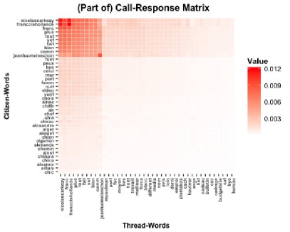
Figure 6: Part of the Call-Response Matrix before and after Thresholding Some pairs of words are relatively more highly correlated, like nicolassarkozy and francoishollande, jeanlucmelenchon and jeanlucmelenchon, vot and franc, etc. After thresholding, only the relatively highly correlated pairs of words are left, making the call-response matrix much more sparse.

Thus, we finally define the matrix that replaces $C$ from CASC. For pairGraphText, define

$$C_{T}=XT_{\omega}(W)Y^{T}.$$ (3.4)

The following diagram reviews how pairGraphText refines the matrix $C$ from CASC.

Note that

$$C_{T}=\sum\limits_{ij}[T_{\omega}(W)]_{ij}X_{\cdotp i}Y_{\cdotp j}^{T}$$

shows closeness of citizens and candidate-posts based on their usage of words in the network. $[C_{T}]_{ij}$ is large when citizen $i$ and candidate-post $j$ use many highly correlated pairs of words. The threshold function $T_{\omega}(\cdotp)$ helps select pairs of words, and imposes sparsity when $W$ is high-dimensional.

Therefore, pairGraphText applies di-sim to the similarity matrix:

$$S=L+hC_{T}.$$ (3.5)

This similarity matrix combines both the graph information, represented by $L$, and the text information, represented by $C_{T}=XT_{\omega}(W)Y^{T}$, with a tuning parameter $h$ to balance between these two parts.

Algorithm 1 pairGraphText

Input: adjacency matrix $A\in\mathbbm{R}^{N_{P}\times N_{C}}$, node covariate matrices $X\in\mathbbm{R}^{N_{P}\times M_{P}}$ and $Y\in\mathbbm{R}^{N_{C}\times M_{C}}$, number of citizen-clusters $K_{C}$, number of post-clusters $K_{P}$, weight $h$, and the significance level $\alpha$.

1. Compute the regularized graph Laplacian $L$ from $A$ as in (3.1). Center $X$ and $Y$ by column. (In practice, scaling $X$ and $Y$ by rows and columns or using weighted $X$ and $Y$ might also be beneficial. See more details in Section 6.2. )

2. Compute $W=X^{T}LY$. Set $\omega$ to be the $1-\alpha$ quantile of $|W_{ij}|$’s.

3. Compute the similarity matrix for pairGraphText as

   $$S=L+hXT_{\omega}(W)Y^{T}.$$

4. Compute the top $K$ left and right singular vectors $U_{C}\in\mathbb{R}^{N_{C}\times K}$, $U_{P}\in\mathbb{R}^{N_{P}\times K}$ corresponding to the $K$ largest singular values of $S$, where $K=\min\{K_{C},K_{P}\}$.

5. Form matrices $U_{C}^{\ast}\in\mathbb{R}^{N_{C}\times K}$ and $U_{P}^{\ast}\in\mathbb{R}^{N_{P}\times K}$ such that for any $i\in\{1,\dots,N_{C}(N_{P})\}$,

   $$[U_{C}^{\ast}]_{i\cdotp}=\frac{[U_{C}]_{i\cdotp}}{\|[U_{C}]_{i\cdotp}\|_{2}}\text{ and }[U_{P}^{\ast}]_{i\cdotp}=\frac{[U_{P}]_{i\cdotp}}{\|[U_{P}]_{i\cdotp}\|_{2}}.$$ (3.6)

6. Cluster the rows of $U_{C}^{\ast}$ into $K_{C}$ clusters with k-means. If the $i$th row of $U_{C}^{\ast}$ falls in the $k$th cluster, assign citizen $i$ to citizen-cluster $k$.

7. Cluster the candidate-posts by performing step 6 on the matrix $U_{P}^{\ast}$ with $K_{P}$ clusters.

4 Issue-centered structure

We identify topics that attract public’s attention in the Facebook discussion threads using pairGraphText. We scale the document-term matrices by both rows and columns. From the scree plot of the singular values of $S$ (see Figure 3 in supplementary material), we decide to study the top $K=4$ clusters due to the large gap after the fourth singular value. To study how the text in discussion threads affects the partition of citizens and candidate-posts, we show the clustering results in three cases: (i) when we use no text, i.e. the tuning parameter $h$ in Equation (3.5) is $h=0$, (ii) when we incorporate text, i.e. $h=0.035$, and (iii) when we only use the text assisted part (defined in $\eqref{def:text_assisted}$), i.e. $h=\infty$.

Section 4.1 shows that with more text incorporated (i.e. with larger $h$), the clusters become less candidate-centered. Section 4.2 introduces a word-content strategy to extract topics of clusters. Section 4.3 describes the cluster topics and supports Section 4.1 by showing that clusters with larger $h$ are more heavily focused on the contextualizing information.

4.1 The clusters from pairGraphText with larger $h$ are less candidate-centered

For each partition of candidate-posts, $\mathcal{P}:\{1,...,N_{P}\}\rightarrow\{1,...,4\}$, we define the matrix $\Psi_{P}\in\mathbbm{R}^{4\times 8}$ such that for any $a\in\{1,...,4\}$ and $b\in\{1,...,8\}$,

$$[\Psi_{P}]_{ab}=\frac{\text{\# of posts in cluster $a$ from candidate $b$'s wall}}{(\text{\# of posts in cluster $a$})\times(\text{\# of posts from candidate $b$'s wall})}.$$ (4.1)

$\Psi_{P}$ shows how post-clusters distribute on candidate-walls. This is similar to $\Psi_{C}$ defined in $\eqref{def:psi_c}$, which shows how citizen-clusters interact with candidate-walls. Figure 7 displays $\Psi_{P}$ and $\Psi_{C}$ in balloon plots in the three cases. When we use no text, i.e. $h=0$, there appears some candidate-centered structure in both citizen-clusters and post-clusters. As we incorporate text, in the case when $h=0.035$, each post-cluster spreads across multiple candidates. With even more text incorporated, in the case $h=\infty$, neither of the post-clusters nor citizen-clusters are candidate-centered. In the following subsections, we identify the cluster topics using key words, comments and posts.

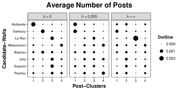
Figure 7: Clusters and Candidate-Walls Figure (a) and (b) display $\Psi_{P}$ and $\Psi_{C}$ in ballloon plots for the three cases.

4.2 A word-content strategy to identify cluster topics

To identify the cluster topics, we first identify keywords for each cluster, which we will define in Section 4.2.1. These keywords give the first impression of the cluster topics.

However, it is insufficient to examine the words in isolation, because the same word is often used differently by different subsets of the population. For example, religion is often used by citizens talking about the religion of peace and it is also often used by atheists criticizing its appearance in the public sphere. Thus, to identify the cluster topics, besides identifying keywords, we also need to read through the conversations that contain these keywords. We focus on the central conversations in each cluster, which we will define in Section 4.2.2.

We call this strategy word-content strategy, where for each cluster, we (i) identify the keywords and (ii) read through the central conversations that contain the keywords in the cluster.

4.2.1 Identify the keywords

We identify the keywords in each cluster by setting “scores”. For any $k\in\{1,\dots,4\}$ and $j\in\{1,\dots,M_{C}\}$, define the score of citizen-word $j$ in citizen-cluster $k$ as

$$\Phi_{kj}=\frac{\sum\limits_{i\in k}X_{ij}}{\sum\limits_{i\in k}\hat{X}_{ij}},\text{ where }\hat{X}_{ij}=\frac{\sum\limits_{j}X_{ij}\sum\limits_{i}X_{ij}}{\sum X_{ij}},$$

and $i\in k$ denotes the citizen $i$ belongs to cluster $k$. We similarly define the scores of thread-words in post-clusters based on the document-term matrix of candidate-posts $Y$. These scores are also discussed in Witten, (2011), where they are derived by maximum likelihood on a Poisson model. We define the keywords in a cluster to be the words with the largest scores in the cluster. We show keywords of each cluster in Section 4.3.

4.2.2 Identifying central conversations

We identify the central conversations by diagnostics from k-means clustering. Recall the pairGraphText algorithm partitions citizens by applying k-means on the $N_{C}$ rows of matrix $U_{C}^{\ast}\in\mathbbm{R}^{N_{C}\times 4}$ (defined in (3.6)) which correspond to the $N_{C}$ citizens. For any citizen $i$, we denote their cluster-centrality as

$$\rho_{i}=[U_{C}^{\ast}]_{i\cdotp}^{T}[\mu_{C}^{\ast}]_{i},$$

where $[\mu_{C}^{\ast}]_{i}$ is the cluster centroid of citizen $i$ from k-means on rows of $U_{C}^{\ast}$. There are four different cluster centroids. For each cluster, the central citizens are the citizens in the cluster with the largest cluster-centrality, i.e. those that align best with the cluster centroid. We similarly define the central posts for post-clusters. For a citizen-cluster, the central conversations are the comments from the central citizens; for a post-cluster, the central conversations are the discussion threads (including posts and comments) initiated by the central posts.

We read through the central conversations that contain the keywords in each cluster. This word-content strategy helps us identify topics that attract citizens’ attention. We will show these topics in Section 4.3.

4.3 Topics of clusters

We extract topics of the clusters by the word-content strategy in three cases, $h=0$, $h=0.035$, and $h=\infty$. Figure 8, 9 and 10 show the cluster topics with the keywords and a brief description of the central conversations in each cluster. In these figures, the links indicate major interactions between citizen-clusters and post-clusters, with the link widths proportional to elements of matrix $\Psi\in\mathbbm{R}^{4\times 4}$, where for any $a,b\in\{1,\dots,4\}$,

$$\Psi_{ab}=\frac{\text{\# of comments from citizens in citizen-cluster $a$ under candidate-posts from post-cluster $b$}}{(\text{\# of citizens in citizen-cluster $a$})\times(\text{\# of candidate-posts in post-cluster $b$})}.$$

This is similar to matrices $\Psi_{C}$ defined in $\eqref{def:psi_c}$ and $\Psi_{P}$ defined in $\eqref{def:psi_p}$, which show how clusters (for citizens or candidate-posts) distribute on the eight candidate-walls. $\Psi$ shows how the citizen-clusters interact with the post-clusters.

When $h=0$ (see Figure 8), clusters focus on candidates or the radical discussions. As we incorporate the text, in the case when $h=0.035$ (see Figure 9), the citizen-clusters are similar to those when $h=0$, but there appears a post-cluster about ecology. As we incorporate more text, in the case when $h=\infty$ (see Figure 10), we identify more topics, such as economic and crises. There also appear a cluster for both citizens and candidate-posts with many copy-paste comments. More data analysis results are in a Shiny App available at https://yilinzhang.shinyapps.io/FrenchElection.

Incorporating the text makes the central conversations more vivid representations of the clusters, allowing for a more precise interpretation of the topic. During the 2012 French election, the citizens devoted their attention and expression in (i) the debates and fights among different candidates, (ii) radical discussions on Islam, religion, and immigration, and (iii) other topics including ecology, economy, and crises.

Figure 8: Cluster topics when $\bm{h=0}$

Figure 9: Cluster patterns when $\bm{h=0.035}$

Figure 10: Cluster patterns when $\bm{h=\infty}$

5 Statistical consistency of pairGraphText

This section shows that our graph contextualization method, pairGraphText, is statistically consistent under the Node Contextualized Stochastic co-Blockmodel (NC-ScBM), which is a fusion of the NC-SBM (Binkiewicz et al., (2017)) and ScBM (Rohe et al., (2016)).

Definition 5.1.

Let $Z_{C}\in\{0,1\}^{N_{C}\times K_{C}}$ and $Z_{P}\in\{0,1\}^{N_{P}\times K_{P}}$, such that there is only one 1 in each row and at least one 1 in each column. Let $B\in[0,1]^{K_{C}\times K_{P}}$ be of rank $K=\min\{K_{C},K_{P}\}$. Let $E_{C}\in\mathbbm{R}^{K_{C}\times M_{C}}$ and $E_{P}\in\mathbbm{R}^{K_{P}\times M_{P}}$. Under the NC-ScBM, the adjacency matrix $A\in\{0,1\}^{N_{C}\times N_{P}}$ contains independent Bernoulli random variables with

$$(1)\quad\mathcal{A}=\mathbbm{E}[A]=Z_{C}BZ_{P},$$

and the node covariate matrices $X\in\mathbbm{R}^{N_{C}\times M_{C}}$ and $Y\in\mathbbm{R}^{N_{P}\times M_{P}}$ contain independent sub-gaussian elements with

$$(2)\quad\mathcal{X}=\mathbbm{E}[X]=Z_{C}E_{C}\text{ and }\mathcal{Y}=\mathbbm{E}[Y]=Z_{P}E_{P}.$$

Recall the similarity matrix for pairGraphText defined in Equation (3.5), $S=L+hXT_{\omega}(W)Y^{T}$. We define the population similarity matrix as

$$\mathcal{S}=\mathcal{L}+h\mathcal{X}\mathcal{W}\mathcal{Y}^{T},$$ (5.1)

where $\mathcal{L}=\mathcal{D}_{C}^{-1/2}\mathcal{A}\mathcal{D}_{P}^{-1/2}$ and $\mathcal{W}=\mathcal{X}^{T}\mathcal{L}\mathcal{Y}$, where diagonal matrices $[\mathcal{D}_{C}]_{ii}=\sum_{j}\mathcal{A}_{ij}+\tau_{c}$ and $[\mathcal{D}_{P}]_{jj}=\sum_{i}\mathcal{A}_{ij}+\tau_{p}$. Let $U_{C}$ and $\mathcal{U}_{C}\in\mathbbm{R}^{N_{C}\times K}$($U_{P}$ and $\mathcal{U}_{P}\in\mathbbm{R}^{N_{P}\times K}$) contain the top $K$ left(right) singular vectors of $S$ and $\mathcal{S}$.

The basic outline of the proof for statistical consistency is: Under some conditions,

1. the element-wise difference between $T_{\omega}(W)$ and $\mathcal{W}$ is bounded by $\omega$ in probability;

2. the similarity matrix $S$ converges to $\mathcal{S}$ in probability;

3. the singular vectors $U_{C}$ and $U_{P}$ converge to $\mathcal{U}_{C}$ and $\mathcal{U}_{P}$ within some rotations in probability;

4. the mis-clustering rates for citizens and candidate-posts goes to zero in probability.

The definition of mis-clustered is the same as in Rohe et al., (2016) and is given in Section 3.2 in supplementary material. The complete proof is given in Section 3.3 in supplementary material.

Denote $\|\cdotp\|$ as the spectral norm and $\|\cdotp\|_{F}$ as the Frobenius norm. For any matrix $H$, we define $sym(H)=\left(\begin{matrix}0&H\\ H^{T}&0\end{matrix}\right)$ and $\|H\|_{2}=\max(\|\max\limits_{i}\|H_{i\cdotp}\|_{2},\max\limits_{j}\|H_{\cdotp j}\|_{2})$. Denote $\|\cdotp\|_{\phi_{2}}$ as the sub-gaussian norm, such that for any random variable $\xi$, there is $\|\xi\|_{\phi_{2}}=\sup\limits_{t\geq 1}t^{-1/2}(\mathbb{E}|\xi|^{t})^{1/t}$. To simplify notation, we denote $N$ as the number of nodes and $M$ as the number of covariates, though $N_{C}$ and $N_{P}$, $M_{C}$ and $M_{P}$ can be different.

Theorem 5.2.

Suppose $A$, $X$ and $Y$, are the adjacency matrix and the node covariate matrices sampled from the NC-ScBM. Let $\lambda_{1}\geq\lambda_{2}\geq\cdots\lambda_{K}>0$ be the $K$ non-zero singular values of $\mathcal{S}$. Let $\mathcal{M}_{C}$ and $\mathcal{M}_{P}$ be the mis-clustered citizens and the mis-clustered candidate-posts. Denote $q_{c}$ and $q_{p}$ as the largest sizes of citizen-clusters and post-clusters. Define $\delta=\min(\min_{i}[\mathcal{D}_{C}]_{ii},\min_{j}[\mathcal{D}_{P}]_{jj})$ and $\gamma=\max(\|X\|_{2},\|Y\|_{2},\|\mathcal{X}\|_{2},\|\mathcal{Y}\|_{2})$. Define $\xi=\max(\sigma^{2}\|L\|_{F}\sqrt{\ln M},\sigma^{2}\|L\|\ln M,\frac{\gamma^{2}}{\delta}\sqrt{\ln M})$, where $L$ is the regularized graph Laplacian defined in Equation (3.1) and $\sigma=\max(\max_{ij}\|X_{ij}-\mathcal{X}_{ij}\|_{\phi_{2}},\max_{ij}\|Y_{ij}-\mathcal{Y}_{ij}\|_{\phi_{2}})$. For any $\epsilon\in(0,1)$, assume

$$(1)\quad\delta>3\ln(2N)+3\ln(8/\epsilon),$$

$$(2)\quad\xi=o(\omega),\text{ and }$$

$$(3)\quad h\leq\min(\frac{a}{\gamma^{2}\|sym(\mathcal{W})\|},\frac{a}{\gamma^{2}\omega})\text{, where }a=\sqrt{\frac{3\ln(16N/\epsilon)}{\delta}}.$$

Then, with probability at least $1-\epsilon$, for large enough $N$, the mis-clustering rates

$$\frac{|\mathcal{M}_{C}|}{N}\leq\frac{c_{0}q_{c}K\ln(16N/\epsilon)}{N\lambda_{K}^{2}\delta}\text{ and }\frac{|\mathcal{M}_{P}|}{N}\leq\frac{c_{0}q_{p}K\ln(16N/\epsilon)}{N\lambda_{K}^{2}\delta},$$

for some constant $c_{0}$.

Remark

Assumption (1) indicates the sparsity of the graph. Assumption (2) and (3) are conditions on parameters $\omega$ and $h$ for consistency. Note the largest sizes of clusters $q_{c}$ and $q_{p}$ are $O(N)$. Suppose $\lambda_{K}$ is lower bounded by some constant $c_{1}>0$, which indicates the “signal” of each of the $K$ blocks is strong enough to be detected. Then, when $\delta$ grows faster than $\ln N$, we have mis-clustering rates goes to zero as $N\rightarrow\infty$.

6 Comparison analysis

Section 6.1 shows the importance of the call-response matrix $W$. Section 6.2 discusses different scaling and weighting choices for document-term matrices. In Section 6.3, we compare pairGraphText with state-of-the-art topic modeling approach, relational topic model (RTM) (Chang and Blei,, 2009), on both the Facebook discussion threads (Section 6.3.1) and on the simulated data (Section 6.3.2).

6.1 Importance of the call-response matrix $W$

Recall the call-response matrix $W$ (defined in (3.2)), which shows the correlation between citizen-words and thread-words on the communication network. It induces weights on different pairs of citizen-words and thread-words; word-pairs with higher correlation on the network are weighted more. In this section, we show the importance of the weights induced by the matrix $W$. We compare pairGraphText with the all-one pairGraphText, which replaces matrix $W$ by the “all-one” matrix, $J\in\mathbbm{R}^{M_{C}\times M_{P}}$, where $J_{ij}=1$, for all $i,j$. For comparison, we set the tunning parameter in (3.5) as $h=\infty$. Table 1 and 2 show the keywords of each cluster by pairGraphText and by all-one pairGraphText.

Table 1: Keywords in clusters by pairGraphText

Citizen-Clusters
Cluster 1	François Hollande, Nicolas Sarkozy,
	fail, president, live, incompetent, May,
	charisma, arrogant, dwarf, goodbye, liar
Cluster 2	residential, descent, child, clinical, chic,
	aristocrat, inhabit, land, employment
Cluster 3	Koran, Allah, religion, Islam, angel,
	pig, pork, Muslim, Arab, racist
Cluster 4	JLM, comrade, resistance, FDG,
	front, Jean-Luc Mélenchon, liberal,
	revolutionary, human, capital, ecologic

Post-Clusters
Cluster 1	concord, flamby, sir, president, captain, bravo,
	charisma, assistantship, arrogant, goodbye,
	strong, debate, failed, incompetent
Cluster 2	employment, euro, child, residential,
	pedigree, chic, clinic, pent, inhabit, land
Cluster 3	Koran, religion, Allah, angel, Islam, pig,
	Muslim, mosque, Arab, Lyon, racist, church
Cluster 4	JLM, comrade, resistance, FDG, troll,
	Jean-Luc Mélenchon, revolutionary, front,
	human, struggle, liberal, fight

Table 2: Keywords in clusters by all-one pairGraphText

Citizen-Clusters
Cluster 1	identity, trick, fascist, opposite, reducer,
	Allah, flamby, top, continuous,
	incarnate, commercial, mission
Cluster 2	baptist, professor, suburb, king,
	happiness,aristocrat, sincerity, school,
	regime, residential, exist, erasable, place
Cluster 3	dismissal, fraud, multiple, lump,
	aggravating, unfair, review, gift,
	parliamentary, budget, referendum
Cluster 4	Parisian, Russian, discriminant,
	defense, land, vineyard, flag, revel,
	pedigree, captain, conceivable,

Post-Clusters
Cluster 1	continued, resistance, great, passion,
	channel, bravo, debate, fight, difficult,
	goodbye, great, beat, stand, hope
Cluster 2	troll, military, comrade, raid, concord, max,
	Philippe Poutou, tomorrow, soldier, killer,
	victim, hateful, bulletin, Jewish, fraud
Cluster 3	Allah, Israel, altarpiece, foul, angel,
	dozen, list, cuckoo, municipal
Cluster 4	lucid, Allah, African, boat, clandestine,
	sister, successful, realist, old, movie,
	angel, tear, promise

Without weights on the word-paris, the all-one pairGraphText fails to extract some topics in the citizen-clusters, such as Islam and the debates among top candidates, which are clear in the citizen-clusters by pairGraphText. Moreover, some words appear in multiple clusters by the all-one pairGraphText. For example, the word Allah appears in both post-cluster 3 and 4 in Table 2. This makes it harder to distinguish different topics between different clusters.

6.2 Different choices for document-term matrices

Recall the document-term matrices $X$ and $Y$ (defined in Section 3.2). These matrices don’t consider lengths of comments and posts or popularities of words. We can address this issue by either (1) scaling the document-term matrices by rows and columns as in Section 4, i.e. replacing $X_{ij}$ and $Y_{ij}$ by

$$X_{ij}/\sqrt{\sum_{i}X_{ij}\sum_{j}X_{ij}}\text{ and }Y_{ij}/\sqrt{\sum_{i}Y_{ij}\sum_{j}Y_{ij}}\text{,}$$

or (2) using the weighted document-term matrices. One standard weighting method is TF-IDF (term frequency-inverse document frequency), which is commonly used in information retrieval and text mining (Salton et al., (1975); Joachims, (1996); Sivic and Zisserman, (2003); Ramos et al., (2003)). TF-IDF weights words based on both the document length and the word popularity. For each word $i$ and document $j$, the TF-IDF is

$$\frac{\text{\# of occurences of word $i$ in document $j$}}{\text{\# of words in document $j$}}\times\log_{2}\frac{\text{\# of documents}}{\text{\# of documents that contain word $i$}}.$$

In our data, documents are the posts and comments in the discussion threads. For the weighted document-term matrix of citizens $Y$, we first calculate the TF-IDF matrix of comments, and then add up those comments from the same citizen. The weighted document-term matrix $X$ is the TF-IDF matrix of posts. We compare plain (unscaled and unweighted), scaled, and TF-IDF weighted document-term matrices on the Facebook discussion threads in Section 3 in the supplementary material.

6.3 Comparison with relational topic model

This section compares pairGraphText and Relational Topic Model(RTM) on both Facebook discussion threads (Section 6.3.1) and simulated data (Section 6.3.2).

6.3.1 Comparison with Relational Topic Model on the Facebook Discussion Threads

Relational topic model (RTM) (Chang and Blei,, 2009) is a popular approach to extract topics from documents with a network structure (e.g. citation network). RTM is designed for uni-partite networks, where there is only one type of nodes. To apply RTM on the bi-partite network with both candidate-posts and citizens, we consider two approaches, (1) symmetrized network (Table 3) and (2) co-occurrence network (Table 4).

We define the symmetrized network as a network with posts and citizens, disregarding the different types of nodes. Recall the adjacency matrix $A\in\mathbbm{R}^{92,226\times 3239}$(defined in 2.1), the adjacency matrix for the symmetrized network is $sym(A)=\left(\begin{matrix}0&A\\ A^{T}&0\end{matrix}\right)$. Table 3 shows the keywords of the four topics by RTM on the symmetrized network. Words such as Nicolas Sarkozy appears in both Cluster 1 and 3, making it hard to distinguish between different topics. The racial topic (Islam, religion, and immigration), which is clear by pairGraphText, is not that clear in Table 3.

We define the co-occurrence network of posts as a network of posts, where the link width is large when the two posts share many citizens who comment frequently on both posts. Similarly, we define the co-occurrence network of citizens as a network of citizens, where the link width is large when the two citizens comment a lot on many same posts. We define the adjacency matrix of the co-occurrence network for posts as $A^{T}A$ and the adjacency matrix of the co-occurrence network for citizens as $AA^{T}$.

Table 4 shows the keywords of the four topics by RTM on the co-occurrence networks. Similarly to pairGraphText, RTM also extracts topics like Islam and religion, debates among top candidates, and economic issues.

Table 3: Keywords in topics by RTM on symmetrized network

Topics
Cluster 1	Nicolas Sarkozy, president, live,
	François Hollande, bravo, France
	courage, all, good, strong, debate
Cluster 2	residential, land, pent, pedigree, clinical,
	inhabit, chic, functional, school,
	conceivable, childhood
Cluster 3	Nicolas Sarkozy, fair, good, other,
	must, polish, can, say, nothing,
	François Bayrou, generation
Cluster 4	fair, good, Jean-Luc Mélenchon,
	nothing, other, speak, share, yes,
	say, generation, front, racist, Muslim

Table 4: Keywords in topics by RTM on co-occurrence networks

Citizen-Topics
Cluster 1	François Hollande, Nicolas Sarkozy,
	France, Jean-Luc Mélenchon, good,
	all, fair, nothing, must, president
Cluster 2	residential, clinic, stock market, live,
	childhood, build, school, free, assembly,
	departure, functional, bourgeois, depend
Cluster 3	Muslim, religion, Islam, speak, racist,
	insult, Arab, Koran, evil, fear, angel
Cluster 4	European, financial, public, undertaken,
	billion, public, budget, advice, bank,
	balance sheet, service, euros, jobs

Post-Topics
Cluster 1	Nicolas Sarkozy, François Hollande,
	social, debate, may, president, victory,
	change, rich, augment, tax, poor, million
Cluster 2	president, franc, sir, live, bravo, all, aim,
	pay, win, good, want, FDG
Cluster 3	Islam, religion, racist, evil, immigrant, Arab,
	insult, Koran, know, from, Jewish, racism
Cluster 4	more, good, France, Jean-Luc Mélenchon,
	all, fair, Nicolas Sarkozy, François Hollande,
	speak, can, politic, generation

6.3.2 Comparison with relational topic model on simulated data

In this section, we use simulation examples to compare pairGraphText and RTM based upon both statistical accuracy and computational running time.

We simulate documents with links and text, then use pairGraphText and RTM to cluster these documents. There are two sources of data, (1) links between documents, i.e. graph, and (2) text in the documents, i.e. text. We compare pairGraphText and RTM in three cases: (1) when both the graph and text contain block information (both signals), (2) when only the graph contains block information (graph signals), and (3) when only text contains block information (text signals). For each of the three cases, we simulate varying levels of signal strength. (See more details on how we define signals in the next paragraph). For each signal level, we simulate 100 random data sets. Each data set consists of 1000 documents and 1000 words in total, with around 200 words and 20 links per document. In this step, we simulate the documents with links and words under a block model with two blocks, each with around 500 documents and around 500 words. (See more details for the block model in the next paragraph). On each data set, we run pairGraphText and RTM to partition the 1000 documents into two clusters. For RTM, we define its estimated cluster label for each document $i$ as $\max\limits_{k}\text{\# of words in document $i$ belongs to block $k$}$.

We simulate all the adjacency matrices (graphs) and the document-term matrices (text) under a Degree Corrected Stochastic Blockmodel (Karrer and Newman,, 2011). Denote $z(i)$ as the block label of any document $i$ and $z_{text}(w)$ as the block label of any word $w$. Under this model, two documents $i$ and $j$ are linked with each other with probability $\theta_{i}\theta_{j}B_{z(i)z(j)}$, and document $i$ contains word $w$ with probability $\theta_{i}\theta_{w}^{text}B_{z(i)z_{text}(w)}^{text}$, where $\theta_{i}$, $\theta_{j}$, $\theta_{w}^{text}$ are degree parameters. The element $B_{uv}$ shows the expected number of links between blocks $u,v$, and the element $B_{uv}^{text}$ shows the expected number of appearances for words in block $v$ in documents in block $u$. We define $B\propto\left(\begin{matrix}0.1&0.1\\ 0.1&0.1\end{matrix}\right)+sig_{g}\left(\begin{matrix}1&0\\ 0&1\end{matrix}\right)$ and $B^{text}\propto\left(\begin{matrix}0.1&0.1\\ 0.1&0.1\end{matrix}\right)+sig_{t}\left(\begin{matrix}1&0\\ 0&1\end{matrix}\right)$, where the graph signal $sig_{g}$ and the text signal $sig_{t}\in{\{1e-1.8,1e-1.6,\dots,1e3\}}$ separately show graph links and words contain how much block information.

For pairGraphText, we set weight $h$ so that the first singular values of the graph Laplacian $L$ and the text assisted part $hC_{T}$ are equal. We choose the threshold $\omega$ to be the 95% quantile of non-zero $|W_{ij}|$’s. We set the number of random starts in the k-means steps (Step 6 and 7 in Algorithm 1) as $10^{4}$. For RTM, we use the function rtm.collapsed.gibbs.sampler in the R package lda. We set the scalar value of the Dirichlet hyperparameter for topic proportions $\alpha=0.001$, the scalar value of the Dirichlet hyperparamater for topic multinomials $\eta=0.1$, the numeric of regression coefficients expressing the relationship between each topic and the probability of link $\beta=(0.5,0.5)$, and the number of sweeps of Gibbs sampling over the entire corpus to make as $num.iterations=1e4$. We set $\alpha$ to be small since we aim to cluster each document to one topic instead of multiple topics. We set the $num.iterations$ large enough so that the likelihood from each document converges.

Figure 11 compares the mis-clustering rate of pairGraphText and RTM. Without text signals (the middle plot), RTM fails to recover block labels even with large graph signals, but pairGraphText recovers block labels with the graph signal over 10. Without graph signals (the right plot), pairGraphText can only recover 90% of block labels, but RTM recovers all block labels, when the text signal is over 0.4. With both graph signals and text signals (the left plot), both methods perform better than the two cases when only one type of signals exists, and both methods can recover block labels with large enough signals.

RTM generalizes the text-based topic modeling method, LDA (Blei et al.,, 2003), to integrate links (graph); it depends more on text and uses links to improve. On the other hand, pairGraphText generalizes the link-based spectral clustering to integrate text; it depends more on links and uses text to improve. From the Figure 11, RTM fails to recover block labels without text signals, but pairGraphText can still recover most block labels without graph signals. Figure 11 also shows that pairGraphText is much faster than RTM.

RTM enables us to predict keywords and citations for new documents (Chang and Blei,, 2009). However, to cluster massive documents into different topics, pairGraphText is a better choice.

See Section 4 in the supplementary material for more simulations comparing pairGraphText with multiple methods including CASC and spectral clustering.

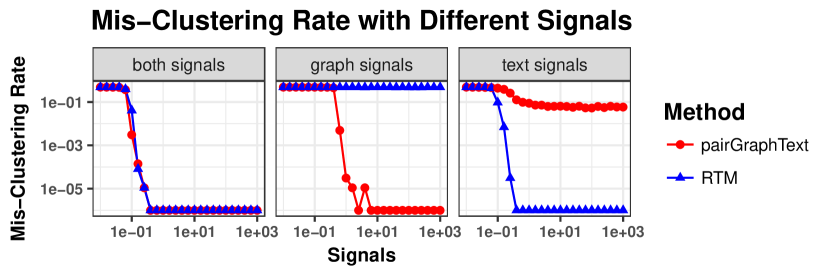
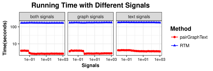
Figure 11: Comparison between pairGraphText and RTM

7 Discussion

This paper searches for (i) candidate-centered structure and (ii) issue-centered structure in the political discussions on Facebook surrounding the 2012 French election. The candidate-centered structure is relatively easy to detect since we have the labels of each post belongs to which candidate. But the search for issue-centered structure is more challenging, because we have no such labels of citizens or any labels of issues. To identify topics in the discussions, we use both the graph and the text. pairGraphText synthesizes the graph and the text, and it adresses the noisy and high-dimensional problem for text by thresholding. Using pairGraphText, we identify topics that attract people’s attention, including Islam, religion, immigration, ecology, economy, and crises. During the interpretation of clusters, we propose the word-content strategy to extract the cluster topics, and our Shiny App https://yilinzhang.shinyapps.io/FrenchElection plays a signicant role in the interdisciplinary collaboration between statisticians and social scientists. Our codes and data sets are available on Github https://github.com/yzhang672/AOAS. We also provide an R package pairGraphText to implement our method on Github https://github.com/yzhang672/pairGraphText.

Chang and Blei, (2010) proposed the relational topic model (RTM), a hierarchical probabilistic model for networks with node covariates. They modeled topic assignments for documents using latent Dirichlet allocation (LDA) (Blei et al., (2003)). Instead of studying networks of documents or posts, we study the bi-partite network between candidate-posts and citizens. Also, our method is unsupervised, more computationally efficient, and generally more accurate compared with RTM. RTM enables us to predict keywords and citations for new documents. However, to cluster documents into different topics, pairGraphText is a better choice than RTM.

pairGraphText is useful for applications outside of discussion threads. It is applicable to any network with node covariates. pairGraphText enhances the homogeneity of covariates within clusters. This boosts the signal of the clusters and helps with interpretation.

References

- Adamic and Glance, (2005) Adamic, L. A. and Glance, N. (2005). The political blogosphere and the 2004 us election: divided they blog. In Proceedings of the 3rd international workshop on Link discovery, pages 36–43. ACM.
- Airoldi et al., (2008) Airoldi, E. M., Blei, D. M., Fienberg, S. E., and Xing, E. P. (2008). Mixed membership stochastic blockmodels. Journal of Machine Learning Research, 9(Sep):1981–2014.
- Bakshy et al., (2015) Bakshy, E., Messing, S., and Adamic, L. A. (2015). Exposure to ideologically diverse news and opinion on facebook. Science, 348(6239):1130–1132.
- Binkiewicz et al., (2017) Binkiewicz, N., Vogelstein, J., and Rohe, K. (2017). Covariate-assisted spectral clustering. Biometrika, 104(2):361–377.
- Blei, (2012) Blei, D. M. (2012). Probabilistic topic models. Communications of the ACM, 55(4):77–84.
- Blei et al., (2003) Blei, D. M., Ng, A. Y., and Jordan, M. I. (2003). Latent dirichlet allocation. Journal of machine Learning research, 3(Jan):993–1022.
- Chang and Blei, (2009) Chang, J. and Blei, D. (2009). Relational topic models for document networks. In Artificial Intelligence and Statistics, pages 81–88.
- Chang and Blei, (2010) Chang, J. and Blei, D. M. (2010). Hierarchical relational models for document networks. The Annals of Applied Statistics, pages 124–150.
- Choy et al., (2011) Choy, M., Cheong, M. L., Laik, M. N., and Shung, K. P. (2011). A sentiment analysis of singapore presidential election 2011 using twitter data with census correction. arXiv preprint arXiv:1108.5520.
- Colleoni et al., (2014) Colleoni, E., Rozza, A., and Arvidsson, A. (2014). Echo chamber or public sphere? predicting political orientation and measuring political homophily in twitter using big data. Journal of Communication, 64(2):317–332.
- Ellison et al., (2007) Ellison, N. B. et al. (2007). Social network sites: Definition, history, and scholarship. Journal of computer-mediated Communication, 13(1):210–230.
- Gonzalez-Bailon et al., (2010) Gonzalez-Bailon, S., Kaltenbrunner, A., and Banchs, R. E. (2010). The structure of political discussion networks: a model for the analysis of online deliberation. Journal of Information Technology, 25(2):230–243.
- Grimmer and Stewart, (2013) Grimmer, J. and Stewart, B. M. (2013). Text as data: The promise and pitfalls of automatic content analysis methods for political texts. Political analysis, 21(3):267–297.
- Hebshi and O’Gara, (2011) Hebshi, S. and O’Gara (2011). The rohe of online social networking in the 2008 democratic presidential primary campains. preprint on webpage at http://www.shoshanahebshi.com/wp-content/uploads/2011/08/Social-Medias-role-in-primary-campaigns.pdf.
- Holland et al., (1983) Holland, P. W., Laskey, K. B., and Leinhardt, S. (1983). Stochastic blockmodels: First steps. Social networks, 5(2):109–137.
- Joachims, (1996) Joachims, T. (1996). A probabilistic analysis of the rocchio algorithm with tfidf for text categorization. Technical report, Carnegie-mellon univ pittsburgh pa dept of computer science.
- Kaplan and Haenlein, (2010) Kaplan, A. M. and Haenlein, M. (2010). Users of the world, unite! the challenges and opportunities of social media. Business horizons, 53(1):59–68.
- Karrer and Newman, (2011) Karrer, B. and Newman, M. E. (2011). Stochastic blockmodels and community structure in networks. Physical review E, 83(1):016107.
- Kim, (2009) Kim, Y. M. (2009). Issue publics in the new information environment: Selectivity, domain specificity, and extremity. Communication Research, 36(2):254–284.
- Kreiss and Mcgregor, (2017) Kreiss, D. and Mcgregor, S. C. (2017). Technology firms shape political communication: The work of microsoft, facebook, twitter, and google with campaigns during the 2016 us presidential cycle. Political Communication, pages 1–23.
- Kushin and Kitchener, (2009) Kushin, M. J. and Kitchener, K. (2009). Getting political on social network sites: Exploring online political discourse on facebook. First Monday, 14(11).
- Pang et al., (2008) Pang, B., Lee, L., et al. (2008). Opinion mining and sentiment analysis. Foundations and Trends® in Information Retrieval, 2(1–2):1–135.
- Papacharissi, (2002) Papacharissi, Z. (2002). The virtual sphere the internet as a public sphere. New media & society, 4(1):9–27.
- Qin and Rohe, (2013) Qin, T. and Rohe, K. (2013). Regularized spectral clustering under the degree-corrected stochastic blockmodel. In Advances in Neural Information Processing Systems, pages 3120–3128.
- Ramage et al., (2009) Ramage, H. R., Connolly, L. E., and Cox, J. S. (2009). Comprehensive functional analysis of mycobacterium tuberculosis toxin-antitoxin systems: implications for pathogenesis, stress responses, and evolution. PLoS genetics, 5(12):e1000767.
- Ramos et al., (2003) Ramos, J. et al. (2003). Using tf-idf to determine word relevance in document queries. In Proceedings of the first instructional conference on machine learning, volume 242, pages 133–142.
- Robertson et al., (2010) Robertson, S. P., Vatrapu, R. K., and Medina, R. (2010). Off the wall political discourse: Facebook use in the 2008 us presidential election. Information Polity, 15(1, 2):11–31.
- Rohe et al., (2016) Rohe, K., Qin, T., and Yu, B. (2016). Co-clustering directed graphs to discover asymmetries and directional communities. Proceedings of the National Academy of Sciences, 113(45):12679–12684.
- Salton et al., (1975) Salton, G., Wong, A., and Yang, C.-S. (1975). A vector space model for automatic indexing. Communications of the ACM, 18(11):613–620.
- Sivic and Zisserman, (2003) Sivic, J. and Zisserman, A. (2003). Video google: A text retrieval approach to object matching in videos. In null, page 1470. IEEE.
- Stieglitz and Dang-Xuan, (2012) Stieglitz, S. and Dang-Xuan, L. (2012). Political communication and influence through microblogging–an empirical analysis of sentiment in twitter messages and retweet behavior. In System Science (HICSS), 2012 45th Hawaii International Conference on, pages 3500–3509. IEEE.
- Stieglitz and Dang-Xuan, (2013) Stieglitz, S. and Dang-Xuan, L. (2013). Social media and political communication: a social media analytics framework. Social Network Analysis and Mining, 3(4):1277–1291.
- Tumasjan et al., (2011) Tumasjan, A., Sprenger, T. O., Sandner, P. G., and Welpe, I. M. (2011). Election forecasts with twitter: How 140 characters reflect the political landscape. Social science computer review, 29(4):402–418.
- Von Luxburg, (2007) Von Luxburg, U. (2007). A tutorial on spectral clustering. Statistics and computing, 17(4):395–416.
- Wang et al., (2012) Wang, H., Can, D., Kazemzadeh, A., Bar, F., and Narayanan, S. (2012). A system for real-time twitter sentiment analysis of 2012 us presidential election cycle. In Proceedings of the ACL 2012 System Demonstrations, pages 115–120. Association for Computational Linguistics.
- Wattal et al., (2010) Wattal, S., Schuff, D., Mandviwalla, M., and Williams, C. B. (2010). Web 2.0 and politics: the 2008 us presidential election and an e-politics research agenda. MIS quarterly, pages 669–688.
- Webster, (2014) Webster, J. G. (2014). The marketplace of attention: How audiences take shape in a digital age. Mit Press.
- Wellman et al., (2001) Wellman, B., Haase, A. Q., Witte, J., and Hampton, K. (2001). Does the internet increase, decrease, or supplement social capital? social networks, participation, and community commitment. American behavioral scientist, 45(3):436–455.
- Williams and Gulati, (2009) Williams, C. B. and Gulati, G. J. (2009). Explaining facebook support in the 2008 congressional election cycle. Working Papers, page 26.
- Williams and Gulati, (2013) Williams, C. B. and Gulati, G. J. (2013). Social networks in political campaigns: Facebook and the congressional elections of 2006 and 2008. New Media & Society, 15(1):52–71.
- Witten, (2011) Witten, D. M. (2011). Classification and clustering of sequencing data using a poisson model. The Annals of Applied Statistics, pages 2493–2518.