Dependence of structure factor and correlation energy on the width of electron wires

Abstract

The structure factor and correlation energy of a quantum wire of thickness $b\ll a_{B}$ are studied in random phase approximation and for the less investigated region $r_{s}<1$. Using the single-loop approximation, analytical expressions of the structure factor have been obtained. The exact expressions for the exchange energy are also derived for a cylindrical and harmonic wire. The correlation energy $\epsilon_{c}$ is found to be represented by $\epsilon_{c}(b,r_{s})=\frac{\alpha(r_{s})}{b}+\beta(r_{s})\;ln(b)+\eta(r_{s})$, for small $b$ and high densities. For a pragmatic width of the wire, the correlation energy is in agreement with the quantum Monte Carlo simulation data.

I Introduction

The motion of electrons confined in one spatial dimension give rise to a variety of interesting phenomena with anomalous propertiesGiuliani05 . Recently quasi one-dimensional systems are experimentally realized in carbon nanotubes Saito98 ; Bockrath99 ; Ishii03 ; Shiraishi03 , semiconducting nanowires Schafer08 ; Huang01 and cold atomic gases Monien98 ; Recati03 ; Moritz05 , edge states in quantum hall liquidMilliken96 ; Mandal01 ; Chang03 and conducting molecules Nitzan03 . The electrons in one dimension do not obey the conventional Fermi-liquid theory, hence the prospect of observation of non-Fermi-liquid features has given a large impetus to both theoretical and experimental research. An appropriate description of the one-dimensional (1D) homogeneous electron gas (HEG) comes from the low-energy theory based on an exactly solvable Tomonaga-Luttinger modelTomonaga50 ; Luttinger63 ; Haldane81 . The random phase approximation (RPA) is the correct theory for HEG in the high-density limit i.e at large electron densities $n=1/(2r_{s}a_{B})$, with $a_{B}$ being the effective Bohr radius and $r_{s}$ is the coupling parameter.

We model the interactions by a smoothed long-range Coulomb potential $v(x)\varpropto(x^{2}+b^{2})^{-1/2}$, where $b$ is a parameter related to the width of the wire. We also use a harmonic confinement potential. The true long-range character of the Coulomb potential has been studied by SchulzSchulz93 and FoglerFogler05a ; Fogler05 using a different approximation than RPA in certain domains of $(b,r_{s})$. In fact a considerable amount of theoretical and numerical work has been done in this domainCapponi00 ; Fano99 ; Poilblanc97 ; Valenzuela03 ; Fabrizio94 ; Friesen80 ; Calmels97 ; Garg08 ; Tas03 ; Renu12 ; Renu14 using RPA and its generalized version, but still there is a need to understand the accurate parametrization of correlation energy for thin wires in the high-density limit. Therefore the calculation of the ground state energy for thin wires in the high-density limit for realistic long-range Coulomb interactions is still an open problem for 1D HEG.

Recently Lee and DrummondLee11 studied the ground state properties of the 1D electron liquid for an infinitely thin wire, and the harmonic wire using the quantum Monte Carlo (QMC) method, and provided a benchmark of the total energy data for a limited range of $r_{s}$. Furthermore, the harmonic wire with transverse confinement has been investigated with a lattice regularized diffusion Monte Carlo (LRDMC) technique by Casula et al. Casula06 , and by othersShulenburger08 ; Malatesta00 ; Malatesta99 .

LoosLoos13 has considered the high-density correlation energy for the 1D HEG using the conventional perturbation theory by taking the smoothed Coulomb potential described above in the limit $b\to 0$ (infinitely thin wire). At $b=0$ they have reported a value of correlation energy at $r_{s}\to 0$ of $-27.4$mHartree per electron. In their calculations the divergences in the integral for small $b$ cancels out exactly. But in RPA the divergences for $b\to 0$ and $r_{s}\to 0$ does not cancel.

The purpose of the present paper is to study electron correlation effects in the interacting electron fluid described by RPA at high densities. The dependence of the structure factor and correlation energy on the wire-width is analyzed in the domain of $r_{s}<1$ and $b\ll a_{B}$. In this respect it is noted that RPA is a vary good approximation in the high density limit $r_{s}\to 0$. We have derived analytical expressions for the static structure factor in the high-density limit. The exact analytical expression for the exchange energy have also been obtained for cylindrical and harmonic potentials. It is found that on the basis of theoretical deduction and a logical assumption, the correlation energy can be represented in this region by the formula $\epsilon_{c}(b,r_{s})=\frac{\alpha(r_{s})}{b}+\beta(r_{s})\;\ln(b)+\eta(r_{s})$, which for small $b\to 0$ disagrees with the result obtained using conventional perturbation theory Loos13 , where it has been found that in the limit of $b\to 0$ and $r_{s}\to 0$, the correlation energy is constant and independent of both.

The paper is organized as follows. In Section II, we calculate the static structure factor within RPA and using the first-order approximation to RPA. In Section III, the RPA ground-state energy formula is given. Subsection III A provides the exact analytical result of exchange energy for cylindrical and harmonic potentials for finite $b$ and $r_{s}$. The result for small-$b$ limit is also given there. Subsection III B describes the correlation energy partially by an analytical formula and partially through numerical calculation. The final result of the correlation energy and its parametrization is presented in section III. In Section IV we discuss the results.

II Structure factor

In this section we calculated the structure factor $S(q)$ within the RPA and its first-order version, where it is possible to obtain the result analytically. The RPA density response function $\chi(q,\omega)$ is given by Pines66 ,

$$\chi(q,\omega)=\frac{\chi_{0}(q,\omega)}{1-V(q)\;\chi_{0}(q,\omega)}$$ (1)

where, $V(q)$ is the Fourier transform of the inter-electronic interaction potential. For harmonically trapped electron wires, and for cylindrical wires it is givenFriesen80 respectively by $V(q)=\frac{e^{2}}{4\pi\epsilon_{0}}~{}E_{1}(b^{2}q^{2})~{}e^{b^{2}q^{2}}$ and $V(q)=2~{}\frac{e^{2}}{4\pi\epsilon_{0}}~{}K_{0}(bq)$, where $E_{1}$ is the exponential integral and $K_{0}$ the modified Bessel function of $2^{nd}$ kind.

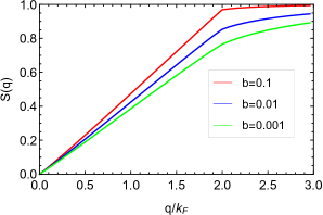
(a)

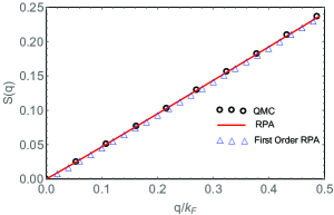
(b)

Figure 1: (Color online) $(a)$ The static structure factor $S(q)$ in RPA for a cylindrical wire is plotted as a function of $q/k_{F}$ for $r_{s}=0.3$, at different thickness of the wire $b$=0.1, 0.01 and 0.001 a.u. $(b)$ the RPA structure factor is compared with diffusion Monte Carlo simulation, and with the first order RPA structure factor for $r_{s}$=0.1 and $b$=0.025.

The static structure factor is defined through the fluctuation-dissipation theorem as

$$S(q)=-\frac{1}{\pi\;n}\int_{0}^{\infty}d\omega\;\chi^{{}^{\prime\prime}}(q,\omega)$$ (2)

where $\chi^{{}^{\prime\prime}}(q,\omega)$ is the imaginary part of the density response function (1). The integral in (2) can be re-written using the contour integration method Giuliani05 as,

$$S(q)=-\frac{1}{\pi\;n}\int_{0}^{\infty}d\omega\;\chi(q,i\omega)$$ (3)

where $n=(k_{F}\;g_{s})/\pi$ is the linear electron number density, $g_{s}$ is the spin degeneracy factor and $k_{F}$ is the Fermi wave vector. Using the high-density expansion

$$\chi(q,i\omega)=\chi_{0}(q,i\omega)+\chi_{0}(q,i\omega)\;V(q)\;\chi_{0}(q,i\omega),$$ (4)

where,

$$\chi_{0}(q,i\omega)=\frac{g_{s}m}{2\pi q}\ln\bigg{[}\frac{\omega^{2}+(\frac{q^{2}}{2m}-\frac{qk_{F}}{m})^{2}}{\omega^{2}+(\frac{q^{2}}{2m}+\frac{qk_{F}}{m})^{2}}\bigg{]},$$ (5)

the structure factor (3) can be calculated for $r_{s}\to 0$ using (4) and (5). The zeroth-order static structure factor is easily calculated

$$S_{0}(q) = -\frac{1}{n\;\pi}\int_{0}^{\infty}\chi_{0}(q,i\;\omega)d\omega$$ (6)

$$= \begin{cases}\frac{q}{2k_{F}},&~{}q<2k_{F}\\[8.61108pt] 1,&~{}q>2k_{F}\end{cases}.$$

The first-order correction to the structure factor can be obtained by substituting $\chi_{0}(q,i\omega)$ in the second term of (4), and than using it in (3). The resulting integral can be performed analytically and we obtain the result for $q<2k_{F}$ as,

$$S_{1}(q)=- v(q)\frac{g_{s}^{2}\;r_{s}\;2k_{F}}{\pi^{2}\;q}\bigg{[}\left(1-{q\over 2k_{F}}\right)\ln\left(1-{q\over 2k_{F}}\right)$$

$$+ \left(1+{q\over 2k_{F}}\right)\ln{\left(1+{q\over 2k_{F}}\right)}\bigg{]}.$$ (7)

Similarly, for $q>2k_{F}$ one obtains

$$S_{1}(q)=- v(q)\frac{g_{s}^{2}\;r_{s}\;2k_{F}}{\pi^{2}\;q}\bigg{[}\left({q\over 2k_{F}}-1\right)\ln\left({q\over 2k_{F}}-1\right)$$

$$+ \left(1+{q\over 2k_{F}}\right)\ln{\left(1+{q\over 2k_{F}}\right)}-{q\over k_{F}}\ln{q\over 2k_{F}}\bigg{]}.$$ (8)

Here and in the following we use $V(q)=v(q)e^{2}/4\pi\epsilon_{0}$. In the limit of small $q$, $q$ around $2k_{F}$ and large $q$, the $S_{1}(q)$ takes the simpler forms given as

$$S_{1}(q)=\begin{cases}-v(q\to 0)\frac{g_{s}^{2}\;r_{s}}{2\pi^{2}}\frac{q}{k_{F}},&~{}q\ll 2k_{F}\\[8.61108pt] -v(q\to 2k_{F})\frac{g_{s}^{2}\;r_{s}}{2\pi^{2}}\frac{k_{F}}{q}\Lambda(z),&~{}q\to 2k_{F}\\[8.61108pt] -v(q\to\infty)\frac{4g_{s}^{2}\;r_{s}}{\pi^{2}}\frac{k_{F}^{2}}{q^{2}},&~{}q\gg 2k_{F}\end{cases}$$ (9)

where $\Lambda(z)=(8\ln(2)-2|z|+2|z|\ln|z|-\frac{3}{4}|z|^{2})$ and $z=\frac{q-2k_{F}}{k_{F}}$. It can be easily seen that for harmonic wires the interaction potential approaches

$$v(q)=\left\{\begin{array}[]{ll}-\gamma-2\ln(bq)~{}~{}\text{for}&\hbox{ bq $\rightarrow$ 0}\\ 1/(bq)^{2}~{}~{}~{}~{}~{}~{}~{}~{}~{}~{}\text{for}&\hbox{ bq $\rightarrow$ $\infty$.}\\ \end{array}\right.$$ (10)

where $\gamma$ is the Euler Gamma constant.

For a cylindrical potential the corresponding results are,

$$v(q)=\left\{\begin{array}[]{lcl}-\gamma+\ln(2)-\ln(bq)&\text{for}&\hbox{ bq $\rightarrow$ 0}\\ e^{-bq}\sqrt{\frac{\pi}{2bq}}&\text{for}&\hbox{ bq $\rightarrow$ $\infty$.}\\ \end{array}\right.$$ (11)

Both potentials behave similarly at the small $bq$ limit, but at large $bq$ they differ. Substituting values of $v(q)$ from (10) in (9), the corresponding leading term agrees with FoglerFogler05 .

To see the effect of thickness $b$ of the wire we calculate the structure factor from (3) by using (1) and (5), for $r_{s}<1$ and plot them in Fig. 1. It is seen from figure 1a that as $b$ decreases, the structure factor $S(q)$ also decreases. A similar trend is also obtained for other $r_{s}$. To see the validity of the first-order structure factor we plot in Fig. 1b for $r_{s}=0.1$, $S_{0}(q)+S_{1}(q)$ and RPA for $b=0.025$. These are compared with diffusion quantum Monte Carlo simulationvinod17 for an infinitely thin wire. All three curves match perfectly. This demonstrate that the system behaves as a gas of non-interacting electrons as conjectured by FoglerFogler05 .

III Ground state energy

The ground-state energy can be obtained by the density-density response function in conjunction with the fluctuation-dissipation theorem as Giuliani05 ,

$$E_{g}=E_{0}+\frac{n}{2}\sum_{q\neq 0}v(q)\bigg{(}-\frac{1}{n\pi}\int^{1}_{0}d\lambda\int^{\infty}_{0}\chi(q,i\omega;\lambda)\;d\omega\bigg{)}.$$

It further simplifies into a sum of kinetic energy of the non-interacting gas with the exchange energy and the residual energy (i.e correlation energy) as,

$$E_{g} = E_{0}+E_{x}+E_{c}$$ (13)

where

$$E_{x} = \frac{n}{2}\sum_{q\neq 0}v(q)\bigg{(}-\frac{1}{n\pi}\int^{1}_{0}d\lambda\int^{\infty}_{0}\chi_{0}(q,i\omega)\;d\omega-1\bigg{)}$$

$$E_{c} = \frac{n}{2}\sum_{q\neq 0}\bigg{(}-\frac{1}{n\pi}\int^{1}_{0}d\lambda\int^{\infty}_{0}\frac{\lambda\;v(q)^{2}\;\chi_{0}^{2}(q,i\omega)}{1-\lambda\;v(q)\;\chi_{0}(q,i\omega)}d\omega\bigg{)}.$$

III.1 Exchange energy

In this section we obtain the exchange energy for a cylindrical as well as for a harmonic electron wire analytically, by integrating (III). Specifically for cylindrical wire it turns out to be,

$$E_{x} = -\frac{Nk_{F}}{\pi}\bigg{(}\frac{-1+2k_{F}b\;K_{1}[2k_{F}b]}{2(k_{F}b)^{2}}+\pi K_{0}[2k_{F}b]$$ (16)

$$\times L_{-1}[2k_{F}b]+\pi K_{1}[2k_{F}b]\;L_{0}[2k_{F}b]\bigg{)}$$

where $K_{n}(x)$ is n^th order modified Bessel function of second kind, and $L_{n}(x)$ is modified Struve functionAbramowitz72 . Similarly, the exchange energy can also be obtained for a harmonic wire of finite thickness given as

$$E_{x} = -\frac{Nk_{F}}{2\pi}\bigg{(}G_{2,3}^{2,2}\left(4b^{2}k_{F}^{2}|\begin{array}[]{c}0,\frac{1}{2}\\ 0,0,-\frac{1}{2}\\ \end{array}\right)$$ (20)

$$-\frac{\ln\left(4b^{2}k_{F}^{2}\right)+e^{4b^{2}k_{F}^{2}}\Gamma\left(0,4b^{2}k_{F}^{2}\right)+\gamma}{4b^{2}k_{F}^{2}}\bigg{)},$$

where $G_{2,3}^{2,2}\left(4b^{2}k_{F}^{2}|\begin{array}[]{c}0,\frac{1}{2}\\ 0,0,-\frac{1}{2}\\ \end{array}\right)$ and $\Gamma\left(0,4b^{2}k_{F}^{2}\right)$ are the Meijer G functionBateman53 and the incomplete gamma function, respectively. For thin harmonic wires $b\ll a_{B}$ the exchange energy can be simplified to be,

$$E_{x} = -\frac{Nk_{F}}{2\pi}\bigg{(}-1-\gamma-\ln(4)-2\ln(k_{F}b)$$ (21)

$$-2\;\psi^{(0)}(1/2)+2\;\psi^{(0)}(3/2)\bigg{)},$$

where $\psi^{(0)}(1/2)$ and $\psi^{(0)}(3/2)$ are polygamma functionsAbramowitz72 . We now use the simpler expansion of the polygamma function as $2\;\psi^{(0)}(1/2)=-2\gamma-2\ln(4)$ and $2\;\psi^{(0)}(3/2)=4-2\gamma-2\ln(4)$ in the above equation. The Eqs.(16) and (20) can also be written for a polarized gas by defining $k_{F_{\uparrow(\downarrow)}}=k_{F}(1\pm p)$, $N_{\uparrow(\downarrow)}=N(1\pm p)/2$ and $k_{F}=\pi/(2g_{s}r_{s}a_{B})$. Explicitly for thin cylindrical wires $b\ll a_{B}$, the exchange energy per particle can be obtained by expanding Eq. (16) as

$$\epsilon_{x} = -\frac{1}{4g_{s}r_{s}}\bigg{(}(1+p)^{2}\bigg{[}\frac{3}{2}-\gamma-\ln\bigg{(}\frac{\pi(1+p)}{2g_{s}r_{s}}\bigg{)}+\mathcal{L}\bigg{]}$$ (22)

$$+(1-p)^{2}\bigg{[}\frac{3}{2}-\gamma-\ln\bigg{(}\frac{\pi(1-p)}{2g_{s}r_{s}}\bigg{)}+\mathcal{L}\bigg{]}\bigg{)}.$$

Similarly for harmonic wires, Eq. (21) gives

$$\epsilon_{x} = -\frac{1}{4g_{s}r_{s}}\bigg{(}(1+p)^{2}\bigg{[}\frac{3}{2}-\frac{\gamma}{2}-\ln(2)-\ln\bigg{(}\frac{\pi(1+p)}{2g_{s}r_{s}}\bigg{)}$$ (23)

$$+\mathcal{L}\bigg{]}+(1-p)^{2}\bigg{[}\frac{3}{2}-\frac{\gamma}{2}-\ln(2)-\ln\bigg{(}\frac{\pi(1-p)}{2g_{s}r_{s}}\bigg{)}$$

$$+\mathcal{L}\bigg{]}\bigg{)},$$

where $\mathcal{L}=\ln(a_{B}/b)$. It is noted that Eqs.(16) and (20) are new results and for special cases noted above they reduce to (22) and (23). It is worth mentioning that the logarithmic thickness of the wire is defined by $\mathcal{L}^{-1}$. For polarized ($g_{s}=1$ and $p=1$) and unpolarized fluids ($g_{s}=2$ and $p=0$), the exchange energy of a cylindrical wire is obtained respectively to be

$$\epsilon_{x}=-\frac{\ln(r_{s})}{r_{s}}-\frac{1}{r_{s}}\bigg{[}\frac{3}{2}-\gamma-\ln(\pi)+\mathcal{L}\bigg{]},$$ (24)

and

$$\epsilon_{x}=-\frac{\ln(4r_{s})}{4r_{s}}-\frac{1}{4r_{s}}\bigg{[}\frac{3}{2}-\gamma-\ln(\pi)+\mathcal{L}\bigg{]}.$$ (25)

These are in agreement with Fogler’s results Fogler05a .

III.2 Correlation energy

Table 1: Parameters obtained in fitting correlation energy data with the formula given in (32) and (33) for various $r_{s}$.

$r_{s}$	Function	$\alpha$	$\beta$	$\eta$	$\chi^{2}$	AdjustedRSquared	AIC	BIC	RSquared
0.1	$\epsilon_{c1}$	-0.500	-5.0	-9.15692	-	-	-	-	-	Fig.2a
	$\epsilon_{c2}$	0.52184	14.9682	54.0315	0.997365	0.998632	291.265	298.579	0.998721	Fig.2a
	$\epsilon_{c}$	-0.000845452	0.319619	1.31095	1	0.999768	-279.783	-272.469	0.999784	Fig.2b
0.01	$\epsilon_{c}$	-0.000378126	-0.032961	-0.119755	1	0.999925	-544.096	-536.781	0.99993	Fig.2c
0.001	$\epsilon_{c}$	-0.0000108161	-0.00244274	-0.0110844	0.937348	0.99788	-333.214	-329.035	0.998183	Fig.2d

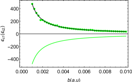
(a)

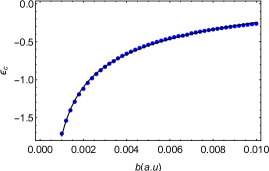
(b)

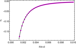
(c)

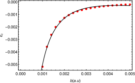
(d)

Figure 2: (color online) $(a)$ The parts of correlation energy $\epsilon_{c1}$ (lower curve) and $\epsilon_{c2}$ (upper curve) versus $b$ for $r_{s}=0.1$ where the analytical result $\epsilon_{c1}$ (green continuous line) are plotted together with the numerical $\epsilon_{c2}$ (green dots) and the fitted curve (black continuous line) for the same $r_{s}$. $(b)$ Total correlation energy $\epsilon_{c}$ for the same value of $r_{s}$ with the fitted curve (black continuous line) and the numerical results (blue dots). $(c)$ and $(d)$ for $r_{s}=0.01$ and $r_{s}=0.001$ respectively, but numerical results (dots) are shown by magenta and red colors.

The integration over the coupling constant $\lambda$ is easily done in (III) and the correlation energy becomes

$$E_{c} = \frac{n}{2}\sum_{q\neq 0}\bigg{(}\frac{1}{n\pi}\int^{\infty}_{0}\{v(q)\;\chi_{0}(q,i\omega)$$ (26)

$$+\ln[1-v(q)\;\chi_{0}(q,i\omega)]\}d\omega\bigg{)}.$$

The above equation can be written further as,

$$\epsilon_{c}=\epsilon_{c1}+\epsilon_{c2}$$ (27)

where

$$\epsilon_{c1} = -\frac{g_{s}}{2\pi}\int^{\infty}_{0}v(q)\;S_{0}(q)\;dq$$ (28)

$$\epsilon_{c2} = \frac{g_{s}}{2\pi}\int^{\infty}_{0}\bigg{(}\frac{1}{n\pi}\int^{\infty}_{0}ln\bigg{\{}1-v(q)\;\chi_{0}(q,i\omega)\bigg{\}}d\omega\ \bigg{)}dq.$$

The first term $\epsilon_{c1}$ can be integrated analytically for the cylindrical potential,

$$\epsilon_{c1} = -\frac{g_{s}^{2}r_{s}a_{B}^{2}}{b^{2}\pi^{2}}+\frac{g_{s}a_{B}}{b\pi}K_{1}\bigg{(}\frac{b}{a_{B}}\frac{\pi}{g_{s}r_{s}}\bigg{)}+\frac{a_{B}}{2br_{s}}$$ (30)

$$\times \bigg{[}-g_{s}r_{s}+\pi(b/a_{B})L_{-1}\bigg{(}\frac{b}{a_{B}}\frac{\pi}{g_{s}r_{s}}\bigg{)}K_{0}\bigg{(}\frac{b}{a_{B}}\frac{\pi}{g_{s}r_{s}}\bigg{)}$$

$$+ \pi bL_{0}\bigg{(}\frac{b}{a_{B}}\frac{\pi}{g_{s}r_{s}}\bigg{)}K_{1}\bigg{(}\frac{b}{a_{B}}\frac{\pi}{g_{s}r_{s}}\bigg{)}\bigg{]}.$$

The Eq. (30) is further simplified for an infinitely thin wire $b\rightarrow 0$ for any finite $r_{s}$ as

$$\epsilon_{c1}=\frac{-g_{s}}{2(b/a_{B})}+\frac{1}{2r_{s}}\bigg{[}\frac{3}{2}-\gamma+\ln\bigg{(}\frac{a_{B}}{b}\bigg{)}-\ln\bigg{(}\frac{\pi}{2g_{s}r_{s}}\bigg{)}\bigg{]}.$$

Table 2: Correlation energy per particle for fully polarized fluids for various $r_{s}$ and $b$.

	correlation energy $\epsilon_{c}$ (mHartree)
$r_{s}$ / b	0.001	0.01	0.1	0.2	0.3	0.4	0.5
0.001	-5.1925	-0.051326	-0.00051321	-0.000128314	-0.000057025	-0.00032081	-0.000205298
0.01	-267.9063	-5.18143	-0.0512140	-0.01280232	-0.00568998	-0.00320059	-0.002048385
0.1	-1675.0533	-258.96748	-5.075932	-1.2577678	-0.5580828	-0.3137399	-0.20074031
0.2	-2250.7232	-568.01835	-19.866556	-4.9634643	-2.1935919	-1.2308436	-0.7868883
0.3	-2543.4151	-684.53832	-41.492422	-11.018708	-4.8636832	-2.7297174	-1.7380320
0.4	-2714.8034	-814.49113	-66.343762	-19.104517	-8.5835144	-4.7704732	-3.0480646
0.5	-2815.2034	-895.4	-93.330872	-28.570889	-13.510079	-7.3493536	-4.6830739

For a given $r_{s}$ the above equation has a functional dependence on $b$ (in atomic unit) as

$$\epsilon_{c1}(b,r_{s})=\frac{\alpha(r_{s})}{b}+\beta(r_{s})\;\ln(b)+\eta(r_{s}),$$ (32)

where $\alpha(r_{s})$, $\beta(r_{s})$ and $\eta(r_{s})$ can be read-off (III.2). Eq.(III.2) cannot be integrated analytically, therefore we solve it numerically. Anticipating that the correlation energy $\epsilon_{c}$ for $b\to 0$ and $r_{s}\to 0$ turns out to be a constant, $\epsilon_{c2}$ may also be represented by (32) with the same coefficient $\alpha(r_{s})$, $\beta(r_{s})$ but with a differing sign and a different constant $\eta(r_{s})$. Therefore we represent $\epsilon_{c2}$ by,

$$\epsilon_{c2}(b,r_{s})=\frac{\alpha(r_{s})}{b}+\beta(r_{s})\;\ln(b)+\eta(r_{s}),$$ (33)

and fit it to the numerical result. The coefficients $\alpha$, $\beta$, $\eta$ for $\epsilon_{c2}$ and $\epsilon_{c}$ are given in Table (1), for $r_{s}$=0.1, 0.01 and 0.001. Note that the coefficients for $\epsilon_{c1}$ are analytically known. Also the same formula as for $\epsilon_{c2}$ is assumed for $\epsilon_{c}$. To estimates the accuracy of the fit with the numerical calculation, we have provided the statistical analysis with different methods: $\chi^{2}$, $R^{2}$ adjusted for the number of model parameters (AdjustedRSquared), Akaike information criterion (AIC), Bayesian information criterion (BIC) and coefficient of determination $R^{2}$ (RSquared). The fitted parameters by the statistical analysis in Table(1) reflect the quality of the function $\epsilon_{c2}(b,r_{s})$ and $\epsilon_{c}(b,r_{s})$.

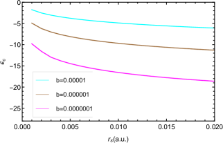
Figure 3: (Color online) The correlation energy per particle is plotted versus $r_{s}$ for different thickness $b$ of cylindrical wire.

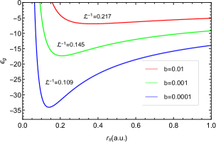
Figure 4: (Color online) Ground state energy $\epsilon_{g}$ is plotted as a function of $r_{s}\leq 1$, for values of wire widths $b$.

The correlation energies per particle $\epsilon_{c1}$ (lower curve) and $\epsilon_{c2}$ (upper curve) are plotted in Fig. 2a, as obtained analytically and numerically, and are shown as green continuous curve and green dots, respectively. The fitted $\epsilon_{c2}$ from representation (33) is shown by the black continuous line. It is clearly seen that there is a perfect fit of $\epsilon_{c2}$, as also inferred above from the statistical analysis. It is seen that there is no cancellation between the two curves for $r_{s}=0.1$. The resulting sum is plotted for the same $r_{s}$ in Fig.2b. Total correlation energy for $r_{s}=0.01$ and $r_{s}=0.001$ are also plotted in Fig. 2c and Fig.2d respectively. These figures show that there is no indication that the correlation energy approaching a constant value for very small $r_{s}$ for an infinitely thin wire. Rather it diverges contrarily to the result obtained by LoosLoos13 as $b$ become vary small.

For a pragmatic width of the wire, the correlation energy for a polarized fluid is reported in Table 1. The correlation energy at high densities $r_{s}\leq 0.1$ and $b=0.1$, is in agreement with the quantum Monte Carlo simulation Casula06 ; Malatesta99 for polarized fluids.

To check the consistency of our result of the correlation energy for $b\to 0$ and $r_{s}<1$, we plot it in Fig. 3 for small values of $b$ shown therein as a function of $r_{s}$. It is seen from Fig. 3 that as $b$ decreases, the correlation energy increases, which is consistent with our previous results given in Figs. 2b , 2c and Fig. 2d.

In Fig. 4 we also plot the total ground-state energy with different wire thicknesses as a function of $r_{s}$. It is noted that as $b$ decreases, the ground state energy increases. There are no QMC data available to compare the ground-state energy for these $r_{s}\ll 1$, for an infinitely thin wire. It is pointed out that our calculation is suited for long-range interactions whereas the Fogler calculation deals with the short-range interaction.

IV Summary

In this paper we have calculated the dependence of the ground-state structure factor and the correlation energy on the thickness of an electron wire as a function of $r_{s}$. The structure factor is calculated in the single-loop approximation of RPA. The electron-electron interactions are modeled by a cylindrical and a harmonic potential. We find an agreement with the result obtained by FoglerFogler05 by a variational calculation. The structure factor has also been compared for $b=0.025$ and $r_{s}=0.1$ with the QMC datavinod17 . For first-order corrections in the interaction, the RPA results and the QMC data match perfectly, indicating that for small thickness and for high densities, the electron gas behaves as a gas of non-interacting particles but highly correlated which is clear from the correlation energy calculations. In this sense FoglerFogler05 ; Fogler05a calls it a Coulomb Tonks gas.

We have also obtained the exchange energy for both cylindrical and harmonic electron wires analytically. These expressions are new. In the small-thickness limit the expressions simplify considerably and are more or less the same for both wires. This has been also worked out for polarized gases, from which the paramagnetic and ferromagnetic phases can easily be obtained. It is also noted that the exchange energy for a fully polarized gas agrees with FoglerFogler05a .

In the present paper the total correlation energy in RPA are found to be fitted by

$$\epsilon_{c}(b,r_{s})=\frac{\alpha(r_{s})}{b}+\beta(r_{s})\;\ln(b)+\eta(r_{s})$$ (34)

with the parameters given explicitly. This correlation energy is the sum of two terms which only partially cancel. The first term is calculated analytically exactly by the expression (34) where the values of $\alpha$, $\beta$ and $\eta$ are precisely known. The second term has been calculated numerically. It perfectly fits with the expression of (34) but with different parameters.

This findings clearly indicate that the correlation energy is diverging in the limit of $b\to 0$ and $r_{s}\to 0$, in contrary to the conventional perturbation theory result Loos13 . Further, the correlation energy as a function of $r_{s}$ for various $b$, again points out that the correlation energy increases as $b$ decreases for $r_{s}\to 0$. The Coulomb correlations are enhanced, and the interacting electron gas behaves structure-less in the ultrathin and high-density domain of $\mathcal{L}^{-1}\ll r_{s}\ll 1$ like a strongly-interacting electron gas named Coulomb-Tonks gas (CTG)Fogler05 ; Fogler05a . Further, we find that the correlation energy does not approach a constant value for an infinitely thin wire and $r_{s}\to 0$ within the RPA.

- (1) G. F. Giuliani and G. Vignale, Quantum theory of the electron liquid (Cambridge University Press, Cambridge, 2005).
- (2) R. Saito, G. Dresselhaus, and M. S. Dresselhaus, Physical Properties of Carbon Nanotubes (Imperial College Press, London, 1998).
- (3) M. Bockrath, D. H. Cobden, J. Lu, A. G. Rinzler, R. E. Smalley, L. Balents, and P. L. McEuen, Nature 397, 598 (1999).
- (4) H. Ishii, H. Kataura, H. Shiozawa, H. Yoshioka, H. Otsubo, Y. Takayama, T. Miyahara, S. Suzuki, Y. Achiba, M. Nakatake, T. Narimura, M. Higashiguchi, K. Shimada, H. Na-matame, and M. Taniguchi, Nature 426, 540 (2003).
- (5) M. Shiraishi and M. Ata, Sol. State Commun. 127, 215 (2003).
- (6) J. Schäfer, C. Blumenstein, S. Meyer, M. Wisniewski, and R. Claessen, Phys. Rev. Lett. 101, 236802 (2008).
- (7) Y. Huang, X. Duan, Y. Cui, L. J. Lauhon, K.-H. Kim, and C. M. Lieber, Science 294,1313 (2001).
- (8) H. Monien, M. Linn, and N. Elstner, Phys. Rev. A 58, R3395 (1998).
- (9) A. Recati, P. O. Fedichev, W. Zwerger, and P. Zoller, J. Opt. B: Quantum Semiclass. Opt. 5, S55 (2003).
- (10) H. Moritz, T. Stoferle, K. Guenter, M. Kohl, and T. Esslinger, Phys. Rev. Lett. 94, 210401 (2005).
- (11) F. P. Milliken, C. P. Umbach, and R. A. Webb, Sol. State Commun. 97, 309 (1996).
- (12) S. S. Mandal and J. K. Jain, Sol. State Commun. 118, 503 (2001).
- (13) A. M. Chang, Rev. Mod. Phys. 75, 1449 (2003).
- (14) A. Nitzan and M. A. Ratner, Science 300, 1384 (2003).
- (15) S. Tomonaga, Prog. Theor. Phys. 5, 544 (1950).
- (16) J. M. Luttinger, J. Math. Phys. 4, 1154 (1963).
- (17) F. D. M. Haldane, J. Phys. C 14, 2585 (1981).
- (18) H. J. Schulz, Phys. Rev. Lett. 71, 1864 (1993).
- (19) M. M. Fogler, Phys. Rev. Lett. 94, 056405 (2005).
- (20) M.M.Fogler, Phys. Rev. B 71, 161304(R)(2005).
- (21) M. Fabrizio, A. O. Gogolin, and S. Scheidl, Phys. Rev. Lett. 72, 2235 (1994).
- (22) S. Capponi, D. Poilblanc, and T. Giamarchi, Phys. Rev. B 61, 13410 (2000).
- (23) G. Fano, F. Ortolani, A. Parola, and L. Ziosi, Phys. Rev. B 60, 15654 (1999).
- (24) D. Poilblanc, S. Yunoki, S. Maekawa, and E. Dagotto, Phys. Rev. B 56, R1645 (1997).
- (25) B. Valenzuela, S. Fratini, and D. Baeriswyl, Phys. Rev. B 68, 045112 (2003).
- (26) W. I. Friesen and B. Bergersen, J. Phys. C 13, 6627 (1980).
- (27) L. Calmels, and A. Gold, Phys. Rev. B 56, 1762 (1997).
- (28) V. Garg, R. K. Moudgil, K. Kumar, and P. K. Ahluwalia, Phys. Rev. B 78, 045406 (2008).
- (29) M. Tas and M. Tomak, Phys. Rev. B 67, 235314 (2003).
- (30) R. Bala, R K Moudgil, Sunita Srivastava and K N Pathak, J. Phys.: Condens. Matter 24 245302 (2012).
- (31) R. Bala, R.K. Moudgil, Sunita Srivastava, and K.N. Pathak, Eur. Phys. J. B 87 5 (2014).
- (32) R. M. Lee and N. D. Drummond, Phys. Rev. B 83, 245114 (2011).
- (33) M. Casula, S. Sorella, and G. Senatore, Phys. Rev. B 74, 245427 (2006).
- (34) A. Malatesta, Quantum monte carlo study of a model one-dimensional electron gas, (Ph.D thesis, Universita Degli studi Di Trieste, Departmento di Fisica Teorica) (1999).
- (35) L. Shulenburger, M. Casula, G. Senatore, and R. M. Martin, Phys. Rev. B 78, 165303 (2008).
- (36) A. Malatesta and G. Senatore, J. Phys. IV 10, 5 (2000).
- (37) P. F. Loos, J. Chem. Phys. 138, 064108 (2013).
- (38) D. Pines and P. Nozieres, The Theory of Quantum Liquids, (W. A. Benjamin, INC. New York, 1966).
- (39) Vinod Ashokan and K.N. Pathak, (2017), (to be published)
- (40) Handbook of mathematical functions, Edited by M. Abramowitz and I. Stegun, Pgs. 498 and 260 (Dover publications, Inc., New York, 1972).
- (41) H. Bateman, A. Erdélyi, Higher Transcendental Functions, Vol. I, (see 5.3, Definition of the G-Function, p. 206) (McGraw Hill, New York, 1953).