An Extensive Study of Bose-Einstein Condensation in Liquid Helium using Tsallis Statistics

Abstract

Realistic scenario can be represented by general canonical ensemble way better than the ideal one, with proper parameter sets involved. We study the Bose-Einstein condensation phenomena of liquid helium within the framework of Tsallis statistics. With a comparatively high value of the deformation parameter $q(\sim 1.4)$, the theoretically calculated value of the critical temperature($T_{c}$) of the phase transition of liquid helium is found to agree with the experimentally determined value ($T_{c}=2.17~{}\rm{K}$), although they differs from each other for $q=1$ (undeformed scenario). This throws a light on the understanding of the phenomenon and connects temperature fluctuation(non-equilibrium conditions) with the interactions between atoms qualitatively. More interactions between atoms give rise to more non-equilibrium conditions which is as expected.

Keywords: Tsallis statistics, Bose-Einstein condensation, liquid helium.

1 Introduction

Statistical mechanics, an important tool in Theoretical Physics, has been successfully used not only in different branch of physics (e.g. condensed matter physics, high energy physics, Astrophysics etc.), but also found to be useful in understanding share price dynamics, traffic control dynamics, etc), hydroclimatic fluctuations, random networks etc. The results predicted by the Statistical Mechanics have been found to be in good agreement with the experiments.

Several attempts have been made to generalize this statistical mechanics in recent years [1, 2, 3, 4, 5, 6] and it (popularly known as superstatistics or $q$-generalized(Tsallis) statistics, where $q$ is the deformation parameter) has already been applied to a wide range of complex systems, e.g., hydrodynamic turbulence, defect turbulence, share price dynamics, random matrix theory, random networks, wind velocity fluctuations, hydroclimatic fluctuations, the statistics of train departure delays and models of the metastatic cascade in cancerous systems [7, 8, 9, 10, 12, 11, 13, 14, 15]. In recent times many authors studied the thermostatic properties of different kind of physical systems(which are more complex than an ideal gas system) like self-gravitating stellar system, Levy flight random diffusion, the galaxy model of the generalized Freeman disk, the electron-plasma 2-$D$ turbulence, the cosmic background radiation, correlated themes, the linear response theory, solar neutrinos, thermalization of electron$-$photon systems etc [16, 17, 18, 19, 20, 21, 22, 23, 24].

This approach deals with the fluctuation parameter $q$ which corresponds to the degree of the temperature fluctuation effect to the concerned system. Here we can treat our normal Boltzmann-Gibbs statistics as a special case of this generalized one, where temperature fluctuation effects are negligible, corresponds to $q=1.0$. More deviation of $q$ from the value $1.0$ denotes a system with more fluctuating temperature. Various works related to this $q$-generalized or Tsallis statistics have been reported in different phenomena [3, 25, 26, 27, 28, 29, 30, 31, 32, 33, 34, 35, 36, 37, 38, 39, 40, 41].

2 Connection between entropy and microstates in Tsallis statistics

A simple connection between the entropy($s$) and the microstates($\Omega$) of a system can be easily derived as $s=k_{B}\ln\Omega$, where one assumes that the entropy($s$) is additive,while the number of microsates($\Omega$) is multiplicative.

A more general connection between $s$ and $\Omega$ can be shown [42, 43] to be equal to

$$s_{q}=k_{B}\ln_{q}\Omega$$ (1)

where the generalized log function($\ln_{q}\Omega$) is defined as

$$\ln_{q}\Omega=\frac{\Omega^{1-q}-1}{1-q}.$$ (2)

Consequently the generalized exponential function becomes

$$e_{q}^{x}=\left[1+(1-q)x\right]^{\frac{1}{1-q}}.$$ (3)

Therefore $q$-modified Shanon entropy takes the following form

$$s_{q}=-k_{B}<\ln_{q}p_{i}>=k\frac{\sum p_{i}^{q}-1}{1-q}$$ (4)

Extremizing $s_{q}$ subject to suitable constraints yields more general canonical ensembles(see B), where the probability to observe a microstate with energy $\epsilon_{i}$ is given by: [1, 44, 45]

$$p_{i}=\frac{e_{q}^{-\beta^{\prime}\epsilon_{i}}}{Z_{q}}=\frac{1}{Z_{q}}\left[1-(1-q)\beta^{\prime}\epsilon_{i}\right]^{\frac{1}{1-q}}$$ (5)

with partition function $z_{q}$ and inverse temperature parameter $\beta=\frac{1}{k_{B}T}$. Also $\beta^{\prime}$ is the $q$-modified quantity and is given by [1, 44]

$$\beta^{\prime}=\frac{\beta}{\sum_{i}p_{i}^{q}+(1-q)\beta u_{q}}=\frac{\beta}{Z_{q}^{1-q}+(1-q)\beta u_{q}}$$ (6)

with $q$-generalized average energy

$$u_{q}=\frac{\sum_{i}\epsilon_{i}p_{i}^{q}}{\sum_{i}p_{i}^{q}}$$ (7)

In the limit of small deformation approximation(i.e., small $\mid 1-q\mid$), $\beta^{\prime}\rightarrow\beta$

3 Bose-Einstein Condensation of liquid $He$ in the framework of $q$-generalized Tsallis Statistics

Whenever a system is subjected to the temperature fluctuation, the non$-$equilibrium generalized statistical mechanics plays a crucial role. If the temperature fluctuation effect is not negligible enough to disclose itself, then it is expected to observe some deviation from the ideal phenomena. Here we study one such phenomena i.e. Bose-Einstein condensation phenomena in Liquid Helium.

The Pauli-Exclusion principle forbids any two fermions to sit at the lowest (or any other value) energy states, while no such principle forbids particles with integral spins to occupy the same quantum states. This gives rise many interesting properties at low temperature and the Bose-Einstein condensation is one of them. With zero spin, a $He^{4}_{2}$ atom is a boson and does not obey the Pauli-Exclusion principle. In 1911, Kamerlingh Onnes first discovered liquid Helium($He^{4}$) at a temperature of $4.2~{}\rm{K}$ [46]. While plotting the specific heat as a function of the temperature for liquid helium $He^{4}_{2}$, Keesom and Clausius in 1932 [47], first found a discontinuity in the specific heat at a temperature $T=2.17~{}\rm{K}$ (called the “critical temperature”) and the specific heat jumped to a large value - a phase transition in which liquid helium goes from its normal phase (i.e. liquid helium phase I) to superfluid phase (liquid helium phase II).

For the liquid helium the theoretically predicted value was $\sim 3.1K$, whereas experiments suggest that the superfluid state of liquid helium has been obtained near $\sim 2.17K$. This happens because the interactions between the atoms are too strong. Only $8\%$ of atoms are in the ground state near absolute zero, rather than the $100\%$ of a true condensate [50, 51, 48, 49].

To study BE-condensation, let us first write down the grand canonical partition function, which in Tsallis statistics, takes the following form:

$$\mathcal{Z}_{q}(T,V,\mu)=\sum_{\left\{n_{k}\right\}=0}^{\infty}\exp_{q}{\left\{-\beta\sum_{k=1}^{\infty}n_{k}\left(\epsilon_{k}-\mu\right)\right\}}$$ (8)

where, $\exp_{q}(x)$ is the $q$-generalized exponential function, given by Eq.(3).

For small deformation (i.e. negligible temperature fluctuation), we find (using Eqs. (37) and (38); please refer to A)

$$\mathcal{Z}_{q} = \sum_{n_{1},n_{2},\cdots=0}^{\infty}\left[\exp_{q}{\left\{-\beta\left(\epsilon_{1}-\mu\right)\right\}}\right]^{n_{1}}\left[\exp_{q}{\left\{-\beta\left(\epsilon_{2}-\mu\right)\right\}}\right]^{n_{2}}\cdots$$ (9)

$$= \prod_{k=1}^{\infty}\sum_{n_{k}=0}^{\infty}\left[\exp_{q}{\left\{-\beta\left(\epsilon_{k}-\mu\right)\right\}}\right]^{n_{k}}$$

$$= \prod_{k=1}^{\infty}\frac{1}{1-z_{q}\exp_{q}{(-\beta\epsilon_{k})}}$$

In above $z_{q}=\exp_{q}(\beta\mu)$ ($\mu$ is the chemical potential) is the $q$-generalized fugacity. The average number of particle(normalized) in $k$-th state(with energy $\epsilon_{k}$)

$$<n_{k}>_{q}=\frac{\sum_{n_{k}=0}^{\infty}n_{k}p_{k}^{q}}{\sum_{n_{k}=0}^{\infty}p_{k}^{q}}$$ (10)

where the probability distribution $p_{k}$ is given by

$$p_{k} = \frac{1}{\mathcal{Z}_{q}}\left[\exp_{q}{\left\{-\beta(\epsilon_{k}-\mu)\right\}}\right]^{n_{k}}$$ (11)

$$= \frac{1}{\mathcal{Z}_{q}}z_{q}^{n_{k}}\exp_{q}(-\beta n_{k}\epsilon_{k})$$

Substituting Eq.(11) into Eq.(10) and simplifying further we get

$$<n_{k}>_{q}=\frac{1}{\left(z_{q}e_{q}^{-\beta\epsilon_{k}}\right)^{-q}-1}$$ (12)

For $q=1$ Eq.(12) exactly replicates the undeformed scenario, which states

$$<n_{k}>=\frac{1}{z^{-1}e^{\beta\epsilon_{k}}-1}$$ (13)

Now the total number of particles (including the ground state)

$$N = \sum_{k}<n_{k}>_{q}$$ (14)

$$= \frac{1}{z_{q}^{-q}-1}+\sum_{k\neq 0}\frac{1}{\left(z_{q}e_{q}^{-\beta\epsilon_{k}}\right)^{-q}-1}$$

$$= N_{0}+N_{\epsilon}$$

with $N_{0}=\frac{1}{z_{q}^{-q}-1}$ and $N_{\epsilon}=\frac{V}{\lambda^{3}}~{}ga_{3/2}(z_{q})$, being the number of particles in the ground state and in the excited states. Here $\lambda(=h/\sqrt{2\pi mk_{B}T}~{})$ is the thermal de-Broglie wavelength and $ga_{3/2}(z_{q})$ is the $q$-generalized polylog function(Bose integral) of the first kind, given by

$$ga_{3/2}(z_{q})=\frac{1}{\Gamma(3/2)}\int_{0}^{\infty}\frac{dx~{}x^{3/2-1}}{\left(z_{q}e_{q}^{-x}\right)^{-q}-1}$$ (15)

$x=\beta\epsilon$ is the dimensionless quantity. Using the expressions in $q$-generalized Tsallis scenario we get the characteristic(i.e. critical) temperature for Bose-Einstein condensation [52] as follows

$$T_{c}=\frac{h^{2}}{2\pi mk_{B}}\left[\frac{n}{ga_{3/2}(z_{q}=1)}\right]^{2/3}$$ (16)

where, $m$ denotes the mass the of the particle species concerned and $n$, the number of the particles per unit volume(i.e. number density(=$N/V$)) respectively. It clearly shows the dependence of $T_{c}$ on the deformation parameter $q$. Below in Fig.[1], we have shown the dependence of the Bose-Einstein condensation temperature ($T_{c}$) on the deformation parameter $q$ for liquid helium[52] (with $n=2.2\times 10^{28}~{}\rm{Atoms/m^{3}}$ and $m=m_{He}=6.8\times 10^{-27}~{}\rm{kg}$).

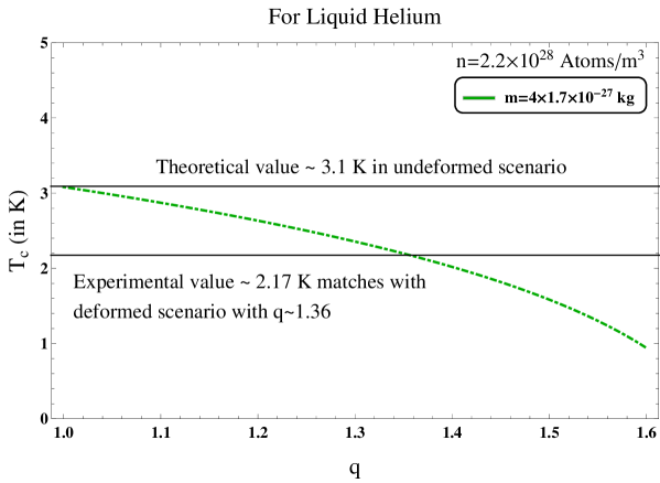
Figure 1: The dependency of the condensation temperature($T_{c}$) for liquid helium on the deformation parameter($q$) is shown.

The upper horizontal curve corresponds to $T_{c}=3.1~{}K$ in undeformed scenario($q=1$), while the lower horizontal curve corresponds to $T_{c}=2.17~{}K$ (the experimental data for liquid hydrogen). The difference between the theoretical prediction and the experimental value of $T_{c}$ for liquid helium can be explained using Tsallis statistics. From the figure we see that the helium condensation temperature $T_{c}$ as predicted by the Tsallis statistics agrees with the experimental value corresponding to $q\sim 1.36$, thereby signifies the importance of deformed statistics which can explain the difference between the theory (undeformed value) and the experiment. In Fig.[2], we have plotted $N_{0}/N$ and $N_{\epsilon}/N$ as a function of $T$ corresponding to $q=1.0,~{}1.1$ and $1.36$ for liquid helium[52].

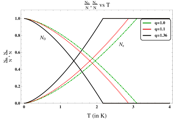
Figure 2: Plots showing the variation of $N_{0}/N$ and $N_{\epsilon}/N$ as a function of $T$ for $q=1.0,~{}1.1$ and $1.36$, respectively. Plots are for liquid helium with $n=2.2\times 10^{28}~{}\rm{Atoms/m^{3}}$ and mass of helium atom is taken to be $m=6.8\times 10^{-27}~{}\rm{kg}$.

From the figure(Fig. 1), we see that as $q$ increases, the critical temperature($T_{c}$) of the Bose-Einstein condensation of liquid helium decreases and eventually matches with the experimental value at $T_{c}=T_{c}^{exp}=2.17~{}\rm{K}$ for the deformation parameter $q=1.36$.

3.1 Specific heat variation and BE condensation

From Eq.9, we find the partition function after simplification,

$$\ln\mathcal{Z}_{q} = \ln\left[\prod_{k=1}^{\infty}\frac{1}{1-z_{q}\exp_{q}{(-\beta\epsilon_{k})}}\right]$$ (17)

$$= \ln(1-z_{q})+\frac{V}{\lambda^{3}}~{}gb_{5/2}(z_{q}),$$

where $gb_{5/2}(z_{q})$ is the $q$-generalized polylog function(Bose integral) of the second kind, given by

$$gb_{5/2}(z_{q})=\frac{1}{\Gamma(5/2)}\int_{0}^{\infty}\frac{dx~{}x^{5/2-1}}{z_{q}^{-1}\left(e_{q}^{-x}\right)^{-q}-\left(e_{q}^{-x}\right)^{1-q}}$$ (18)

The internal energy $U_{q}$($q$-generalized internal energy) is given by [1, 2]

$$U_{q}=-\frac{\partial}{\partial\beta}\ln_{q}\mathcal{Z}_{q}=-\frac{\partial}{\partial\beta}\ln_{q}e^{\ln\mathcal{Z}_{q}}$$ (19)

where the $q$-generalized logarithm is defined by Eq.(2). The normalized $q$-generalized internal energy is defined as [1, 53, 54]

$$<U_{q}>=\frac{U_{q}}{\sum_{i}p_{i}^{q}}=\frac{3}{2}\frac{V}{\lambda^{3}}k_{B}T~{}gb_{5/2}(z_{q})$$ (20)

In BE condensation phase(i.e., $T<T_{c}$), the fugacity $z_{q}=1$. So in this phase the molar specific heat capacity of the system at constant volume is given by

$$C_{V}=\left[\frac{\partial<U_{q}>}{\partial T}\right]_{N,V}=\frac{3}{2}Vk_{B}~{}gb_{5/2}(z_{q}=1)\frac{\partial}{\partial T}\left(\frac{T}{\lambda^{3}}\right)$$ (21)

Now using the fact that $\frac{\partial}{\partial T}\left(\frac{T}{\lambda^{3}}\right)=\frac{5}{2}\frac{1}{\lambda^{3}}$, we find

$$\frac{C_{V}}{Nk_{B}}=\frac{15}{4}\frac{V}{N}\frac{1}{\lambda^{3}}~{}gb_{5/2}(z_{q}=1)\propto T^{3/2}$$ (22)

with $T<T_{c}$ (in condensation phase). For $T>T_{c}$, $z_{q}<1$ and $N_{0}\approx 0$.

$$\therefore N \approx \frac{V}{\lambda^{3}}~{}ga_{3/2}(z_{q})\implies\frac{V}{\lambda^{3}}=\frac{N}{ga_{3/2}(z_{q})}$$ (23)

From Eq.(20)

$$<U_{q}> = \frac{3}{2}\frac{N}{ga_{3/2}(z_{q})}k_{B}T~{}gb_{5/2}(z_{q})=\frac{3}{2}Nk_{B}T~{}\frac{gb_{5/2}(z_{q})}{ga_{3/2}(z_{q})}$$ (24)

and

$$\frac{C_{V}}{Nk_{B}} = \frac{1}{Nk_{B}}\left[\frac{\partial<U_{q}>}{\partial T}\right]_{N,V}$$ (25)

$$= \frac{3}{2}\left[\frac{gb_{5/2}(z_{q})}{ga_{3/2}(z_{q})}+T\frac{\partial}{\partial T}\left\{\frac{gb_{5/2}(z_{q})}{ga_{3/2}(z_{q})}\right\}\right]$$

$$= \frac{3}{2}\left[\frac{gb_{5/2}(z_{q})}{ga_{3/2}(z_{q})}+T\frac{\partial z_{q}}{\partial T}\frac{\partial}{\partial z_{q}}\left\{\frac{gb_{5/2}(z_{q})}{ga_{3/2}(z_{q})}\right\}\right]$$

Now using $\frac{\partial}{\partial T}\left(\lambda^{3}\right)=-\frac{3}{2}\frac{\lambda^{3}}{T}$ and Eq.(23) we get

$$\frac{\partial z_{q}}{\partial T}=-\frac{3}{2}\frac{1}{T}\frac{ga_{3/2}(z_{q})}{ga^{\prime}_{3/2}(z_{q})}$$ (26)

where, $ga^{\prime}_{3/2}(z_{q})$ denotes the derivative of $ga_{3/2}(z_{q})$ with respect to $z_{q}$. Putting this back on Eq.(25) the expression for the molar specific heat capacity per unit volume becomes

$$\frac{C_{V}}{Nk_{B}} = \frac{3}{2}\left[\frac{gb_{5/2}(z_{q})}{ga_{3/2}(z_{q})}-\frac{3}{2}\frac{ga_{3/2}(z_{q})}{ga^{\prime}_{3/2}(z_{q})}\frac{\partial}{\partial z_{q}}\left\{\frac{gb_{5/2}(z_{q})}{ga_{3/2}(z_{q})}\right\}\right]$$ (27)

Simplifying further we get

$$\frac{C_{V}}{Nk_{B}} = \frac{15}{4}\frac{gb_{5/2}(z_{q})}{ga_{3/2}(z_{q})}-\frac{9}{4}\frac{gb^{\prime}_{5/2}(z_{q})}{ga^{\prime}_{3/2}(z_{q})}$$ (28)

Eq.(28) is valid for $T>T_{c}$. For the BE condensation phase in which $T<T_{c}$, the simplified form of Eq.(22) becomes

$$\frac{C_{V}}{Nk_{B}}=\frac{15}{4}\frac{gb_{5/2}(z_{q}=1)}{ga_{3/2}(z_{q}=1)}\left(\frac{T}{T_{c}}\right)^{3/2}$$ (29)

Finally, using the definition of $T_{c}$, Eq.(16) we get

$$\frac{1}{\lambda^{3}}=\left(\frac{T}{T_{c}}\right)^{3/2}\frac{N/V}{ga_{3/2}(z_{q}=1)}$$ (30)

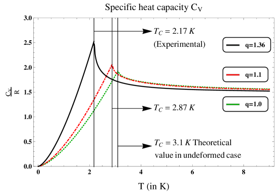
Figure 3: The specific heat $C_{V}/R$ is plotted against $T$ for liquid helium. The plots show the phase transition of liquid helium from its normal phase to it superfluid phase. The plots are shown for $q=1.0,~{}q=1.1$ and $1.36$, respectively.

In Fig.[3], we have plotted the specific heat $C_{V}/R$ (of liquid helium) as a function of $T$ corresponding to the different values of the deformation parameter $q$. We vary $q$ varies from $q=1$ to $q=1.36$ for liquid helium[52] with $n=2.2\times 10^{28}~{}\rm{Atoms/m^{3}}$. The discontinuity (at the peak) in $C_{V}/R$ vs $T$ curve corresponds to the phase transition i.e. transition from normal phase(phase I) to superfluid phase(phase II). We see that as $q$ increases from $1.0$ to $1.36$, the transition temperature $T_{c}$ changes from $3.1~{}\rm{K}$ to $2.17~{}\rm{K}$ which is the experimentally determined value.

A significant amount of work has already been done to observe the effect of generalized Tsallis statistics on the phenomena of Bose-Einstein condensation [55, 56, 57, 58]. Ou et al.studied the thermostatic properties of a $q$-generalized Bose system trapped in an $n$-dimensional harmonic oscillator potential [57] whereas Chen et al.investigated $q$-generalized Bose-Einstein condensation based on Tsallis entropy [58]. Both of the above mentioned works deal with a $D$-dimensional $q$-generalized ideal boson system with the general energy spectrum

$$\varepsilon=ap^{s}$$ (31)

with two positive constants $a$ and $s$. For non-relativistic particle system $a=\frac{1}{2m}$ and $s=2$(where $m$ is the mass of the concerned particle) whereas for relativistic system, $s=1$ and $a=c$(the speed of light).

For $q>1$ they Ou et al.and Chen et al.obtained $q$-generalized Bose integral as follows [57, 58]

$$g_{q,n}(z_{q})=\sum_{j=1}^{\infty}\frac{z_{q}^{j-(1-q)n}}{(q-1)^{n}}\frac{\Gamma(j/(q-1)-n)}{\Gamma(j/(q-1))}$$ (32)

Consequently the $q$-generaized Riemann Zeta function was defined as

$$\zeta_{q}(n)=\sum_{j=1}^{\infty}\frac{1}{(q-1)^{n}}\frac{\Gamma(j/(q-1)-n)}{\Gamma(j/(q-1))},~{}~{}q>1$$ (33)

with the interesting fact that

$$\lim_{q\rightarrow 1}\zeta_{q}(n)=\zeta(n)$$ (34)

Using these facts we can estimate the characteristic(i.e. critical) temperature for Bose-Einstein condensation in $q$-generalized Tsallis scenario which can be expressed as a simple relation now [57, 58]

$$\frac{T_{q,c}}{T_{c}}=\left\{\frac{\zeta(D/s)}{\zeta_{q}(D/s)}\right\}^{s/D}$$ (35)

where $T_{q,c}$ and $T_{c}$ are the Bose-Einstein condensation temperature for $q>1$ and $q=1$ respectively. For a 3 dimensional non-relativistic particle system(as considered in our present work Sec. 3) $s=2$ and $D=3$. In that case, Eq.(35) becomes

$$T_{q,c}=T_{c}\left\{\frac{\zeta(3/2)}{\zeta_{q}(3/2)}\right\}^{2/3}$$ (36)

Now we know that, for $q=1$, $T_{c}=3.1$. Putting $q=1.36$ into the Eq.(36) yields $T_{q,c}=2.178$ which is in nice agreement with the value of the condensation temperature obtained using Eq.(16) for $q=1.36$. Also the most important fact is that for $q=1.36$, both of the Eqs.(36) and (16) giving us a unique theoretical value(in $q$-generalized Tsallis scenario) of the characteristic(i.e. critical) temperature for Bose-Einstein condensation which also agrees with the experimentally determined one.

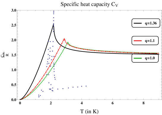
Figure 4: The specific heat $C_{V}/R$ is plotted against $T$ for liquid helium. The plots are shown for $q=1.0,~{}q=1.1$ and $1.36$, respectively with the experimental data points(blue dots) of $C/R$ by Keesom et al.[59].

In Fig.[4], we have plotted the specific heat $C_{V}/R$ (of liquid helium) as a function of $T$ corresponding to the different values of the deformation parameter $q$. Also the experimental data points have been shown which was obtained by W. H. Keesom and A. P. Keesom [59].

4 Conclusion

We study the Bose-Einstein condensation phenomena within the framework of Tsallis statistics. We find that the critical temperature($T_{c}$) of the Bose-Einstein condensation depends strongly on the deformation parameter $q$. For $q=1$ (undeformed scenario), we find that the theoretically calculated value of the critical temperature ($\sim 3.1~{}\rm{K}$) differs from the experimentally measured value $\sim 2.17~{}\rm{K}$. With a relatively high value of the deformation parameter $q$($\sim 1.36$), the theoretical prediction of the critical temperature for liquid helium(which is a highly interacting non-ideal boson system) matches with the experimentally determined one. Here we can consider the deformation parameter $q$ is taking care of the concerned non-equilibrium conditions which arises due to the nearest neighbour interactions among the atoms involved. Consequently the undeformed scenario($q=1.0$, in which we consider an ideal non-interacting bosonic system) failed to explain the discrepancy between the theoretical and the experimentally determined value.

Appendix A Indicial properties of $q$-generalized exponential function for small deformation

From Eq.(3), keeping only first order in $(1-q)$,

$$e_{q}^{a}\cdot e_{q}^{b} = \left[1+(1-q)a\right]^{\frac{1}{1-q}}\cdot\left[1+(1-q)b\right]^{\frac{1}{1-q}}$$ (37)

$$= \left[1+(1-q)(a+b)+(1-q)^{2}ab\right]^{\frac{1}{1-q}}$$

$$\simeq e_{q}^{a+b}$$

Similarly, neglecting higher order terms we get,

$$\left(e_{q}^{a}\right)^{b} = \left[1+(1-q)a\right]^{\frac{b}{1-q}}$$ (38)

$$= \left[1+(1-q)ab+\frac{b(b-1)}{2!}(1-q)^{2}a^{2}+\cdots\right]^{\frac{1}{1-q}}$$

$$\approx e_{q}^{ab}$$

Though in our present discussion, the $q$-value used to fit the data is $q\approx 1.36$, the approximation still holds because of the values of $a$ and $b$ to be substituted in Eqs. (37) and (38). Eqs. (8) and (10) are leading to Eqs. (9) and (12), respectively. There we are using the energy of the particle in $k$-th state as $\epsilon_{k}$ and the $q$-generalized fugacity as $z_{q}=\exp_{q}(\beta\mu)$ with $\mu$ as the chemical potential. The quantities $\beta\mu$ and $\beta\epsilon_{k}$ are to be treated as $a$ and $b$ in Eqs. (37) and (38) to apply the weak deformation approximation(i.e., $\mid 1-q\mid$). The validity of the approximation holds as the quantities associated with $(1-q)^{2}$(or higher order of $(1-q)$) is small like $ab,a^{2}b,a^{2}b^{2}$ etc. (i.e., $\beta^{2}\epsilon_{i}\epsilon_{j},\beta^{3}\epsilon_{i}^{2}\epsilon_{j},\beta^{4}\epsilon_{i}^{2}\epsilon_{j}^{2},\beta^{2}\epsilon_{i}\mu$ etc.). For $q\approx 1.36$, $(1-q)^{2}\approx 0.13$ which is almost $\frac{1}{3}$rd of its first order $(1-q)=0.36$. Clearly we can restrict our consideration up to first order of $\mu$ and $\epsilon_{k}$ with weak deformation approximation. So even for $q\approx 1.36$ the weak deformation approximation is reasonably valid as the contribution of the higher order terms in Eqs. (37) and (38) becomes negligible.

Appendix B Constraints and Entropy Optimization in Tsallis Statistics

To impose the mean value of a variable in addition to satisfy the following fact

$$\int_{0}^{\infty}dx~{}p(x)=1$$ (39)

$q$-generalized mean value of a variable $x$ is to be defined as [1, 44]

$$<x>_{q}=\int_{0}^{\infty}dx~{}xP(x)=X_{q}$$ (40)

whereas, $P(x)$ is the Escort distribution and is defined as

$$P(x)=\frac{[p(x)]^{q}}{\int_{0}^{\infty}dx^{\prime}~{}[p(x^{\prime})]^{q}}$$ (41)

We immediately verify that $P(x)$ is normalized as well

$$\int_{0}^{\infty}dx~{}P(x)=\frac{\int_{0}^{\infty}dx~{}[p(x)]^{q}}{\int_{0}^{\infty}dx^{\prime}~{}[p(x^{\prime})]^{q}}=1$$ (42)

We can use these facts to optimize the generalized entropy $s_{q}$. In order to use the Lagrange’s undetermined multiplier method to find the optimized distribution we define the following quantity

$$\Phi[p]=\frac{1-\int_{0}^{\infty}dx~{}[p(x)]^{q}}{q-1}-\alpha_{q}\int_{0}^{\infty}dx~{}p(x)-\beta_{q}\frac{\int_{0}^{\infty}dx~{}x[p(x)]^{q}}{\int_{0}^{\infty}dx~{}[p(x)]^{q}}$$ (43)

with $\alpha_{q}$ and $\beta_{q}$ as the Lagrange parameters. Therefore imposing the optimization conditions

$$\frac{\partial\Phi(p)}{\partial p}=0$$ (44)

Simplifying further we get

$$p(x)=\frac{e_{q}^{-\beta_{q}\left(x-X_{q}\right)}}{\int_{0}^{\infty}dx^{\prime}~{}e_{q}^{-\beta_{q}\left(x^{\prime}-X_{q}\right)}}$$ (45)

Now from the following two constraints

• $\sum_{i}p_{i}=1$ (Norm constraint)

• $<\epsilon>_{q}=\sum_{i}\epsilon_{i}P_{i}=u_{q}$ (Energy constraint)

  with $P_{i}=\frac{p_{i}^{q}}{\sum_{j}p_{j}^{q}}$

we obtain the distribution as follows

$$p_{i}=\frac{e_{q}^{-\beta_{q}\left(\epsilon_{i}-u_{q}\right)}}{\bar{z}_{q}}$$ (46)

with $\bar{z}_{q}=\sum_{i}e_{q}^{-\beta_{q}\left(\epsilon_{i}-u_{q}\right)}$ and $\beta_{q}=\frac{\beta}{\sum_{j}p_{j}^{q}}$.

Now

$$s_{q} = -k_{B}<\ln_{q}p_{j}>$$

$$= k_{B}\frac{\sum_{j}p_{j}^{q}-1}{1-q}$$

$$\implies\sum_{j}p_{j}^{q} = 1+(1-q)\frac{s_{q}}{k_{B}}$$ (47)

Also

$$s_{q}=-k_{B}\ln_{q}\bar{z}_{q}=\frac{k_{B}}{1-q}\left(\bar{z}_{q}^{1-q}-1\right)$$ (48)

$$\therefore\sum_{j}p_{j}^{q}=1+(1-q)\frac{\frac{k_{B}}{1-q}\left(\bar{z}_{q}^{1-q}-1\right)}{k_{B}}=\bar{z}_{q}^{1-q}$$ (49)

So now

$$\beta_{q}=\frac{\beta}{\sum_{j}p_{j}^{q}}=\beta\bar{z}_{q}^{q-1}$$ (50)

More useful and the convenient form of Eq.(46) for application purpose, is given by [1, 44]

$$p_{i}=\frac{e_{q}^{-\beta^{\prime}\epsilon_{i}}}{Z_{q}}$$ (51)

with $Z_{q}=\sum_{i}e_{q}^{-\beta^{\prime}\epsilon_{i}}$ and $\beta^{\prime}=\frac{\beta_{q}}{1+(1-q)\beta_{q}u_{q}}=\frac{\beta}{Z_{q}^{1-q}+(1-q)\beta u_{q}}$.

Appendix C Converting summations to integrals

Using Eq. (12) we can calculate the total number of particles (including the ground state) in the following way

$$N = \sum_{k}<n_{k}>_{q}$$ (52)

$$= \frac{1}{z_{q}^{-q}-1}+\sum_{k\neq 0}\frac{1}{\left(z_{q}e_{q}^{-\beta\epsilon_{k}}\right)^{-q}-1}$$

$$= N_{0}+N_{\epsilon}$$

where the number of particles in the ground state

$$N_{0}=\frac{1}{z_{q}^{-q}-1}$$ (53)

and the number of particles in the excited states is given by

$$N_{\epsilon}=\sum_{k\neq 0}\frac{1}{\left(z_{q}e_{q}^{-\beta\epsilon_{k}}\right)^{-q}-1}$$ (54)

Converting the above mentioned summation into integral with proper phase-space factor we get

$$N_{\epsilon}=\frac{2\pi V}{h^{3}}(2mk_{B}T)^{\frac{3}{2}}\Gamma(3/2)\frac{1}{\Gamma(3/2)}\int_{0}^{\infty}\frac{dx~{}x^{1/2}}{\left(z_{q}e_{q}^{-x}\right)^{-q}-1}$$ (55)

with $x=\beta\epsilon$ (a dimensionless quantity). The extra factor $(k_{B}T)^{\frac{3}{2}}$ arises due to this change of variable inside the integral. Now $\frac{h}{\sqrt{2\pi mk_{B}T}}=\lambda$, the thermal de-Broglie wavelength and $\Gamma(3/2)=\frac{\sqrt{3}}{2}$.

$$\therefore\frac{2\pi}{h^{3}}(2mk_{B}T)^{\frac{3}{2}}\Gamma(3/2)=\frac{1}{\lambda^{3}}$$ (56)

and

$$N_{\epsilon}=\frac{V}{\lambda^{3}}~{}ga_{3/2}(z_{q})$$ (57)

$ga_{3/2}(z_{q})$ is the $q$-generalized polylog function(Bose integral) of the first kind, given by

$$ga_{3/2}(z_{q})=\frac{1}{\Gamma(3/2)}\int_{0}^{\infty}\frac{dx~{}x^{3/2-1}}{\left(z_{q}e_{q}^{-\beta\epsilon_{k}}\right)^{-q}-1}$$ (58)

Similarly from Eq.9, we get the following

$$\ln\mathcal{Z}_{q} = \ln\left[\prod_{k=1}^{\infty}\frac{1}{1-z_{q}\exp_{q}{(-\beta\epsilon_{k})}}\right]$$ (59)

$$= \ln 1-\ln\left\{1-z_{q}e_{q}^{-\beta\epsilon_{1}}\right\}-\ln\left\{1-z_{q}e_{q}^{-\beta\epsilon_{2}}\right\}-\cdots\infty$$

$$= \ln(1-z_{q})-\sum_{k=0}^{\infty}\ln\left\{1-z_{q}e_{q}^{-\beta\epsilon_{k}}\right\}$$

And after converting the summation into the integral(following the same procedure mentioned above) we get

$$\ln\mathcal{Z}_{q}=\ln(1-z_{q})+\frac{V}{\lambda^{3}}~{}gb_{5/2}(z_{q}),$$ (60)

where $gb_{5/2}(z_{q})$ is the $q$-generalized polylog function(Bose integral) of the second kind, given by

$$gb_{5/2}(z_{q})=\frac{1}{\Gamma(5/2)}\int_{0}^{\infty}\frac{dx~{}x^{5/2-1}}{z_{q}^{-1}\left(e_{q}^{-x}\right)^{-q}-\left(e_{q}^{-x}\right)^{1-q}}$$ (61)

Intermediate steps:

$$-\sum_{k=0}^{\infty}\ln\left\{1-z_{q}e_{q}^{-\beta\epsilon_{k}}\right\} = -\frac{2\pi V}{h^{3}}(2m)^{3/2}\int_{0}^{\infty}\epsilon^{1/2}\ln\left(1-z_{q}e_{q}^{-\beta\epsilon}\right)d\epsilon$$ (62)

$$= -\frac{2\pi V}{h^{3}}(2m)^{3/2}\Biggl{[}\ln\left(1-z_{q}e_{q}^{-\beta\epsilon}\right)\frac{\epsilon^{3/2}}{3/2}\bigl{|}_{0}^{\infty}$$

$$- \int_{0}^{\infty}\frac{z_{q}\beta\left(e_{q}^{-\beta\epsilon}\right)^{q}}{1-z_{q}e_{q}^{-\beta\epsilon}}\frac{\epsilon^{3/2}}{3/2}d\epsilon\Biggr{]}$$

For $\epsilon\rightarrow 0$, $\epsilon^{3/2}=0$ and for $\epsilon\rightarrow\infty$, $\ln\left(1-z_{q}e_{q}^{-\beta\epsilon}\right)=\ln(1-0)=0$

$$\therefore-\sum_{k=0}^{\infty}\ln\left\{1-z_{q}e_{q}^{-\beta\epsilon_{k}}\right\} = -\frac{2\pi V}{h^{3}}(2m)^{3/2}\left[-\int_{0}^{\infty}\frac{z_{q}\beta\left(e_{q}^{-\beta\epsilon}\right)^{q}}{1-z_{q}e_{q}^{-\beta\epsilon}}\frac{\epsilon^{3/2}}{3/2}d\epsilon\right]$$ (63)

$$= \frac{2\pi V}{h^{3}}(2m)^{3/2}\frac{2\beta}{3}\int_{0}^{\infty}\frac{\epsilon^{3/2}~{}d\epsilon}{z_{q}^{-1}\left(e_{q}^{-x}\right)^{-q}-\left(e_{q}^{-x}\right)^{1-q}}$$

$$= \frac{2\pi V}{h^{3}}(2m)^{3/2}\frac{2\beta}{3}\frac{1}{\beta^{5/2}}\int_{0}^{\infty}\frac{x^{3/2}~{}dx}{z_{q}^{-1}\left(e_{q}^{-x}\right)^{-q}-\left(e_{q}^{-x}\right)^{1-q}}$$

$$= \frac{2\pi V}{h^{3}}(2mk_{B}T)^{3/2}\frac{2}{3}\Gamma(5/2)~{}gb_{5/2}(z_{q})$$

$$= \frac{2\pi V}{h^{3}}(2mk_{B}T)^{3/2}\frac{2}{3}\frac{3}{2}\frac{\sqrt{\pi}}{2}~{}gb_{5/2}(z_{q})$$

$$= \frac{V}{\lambda^{3}}~{}gb_{5/2}(z_{q})$$

where $x=\beta\epsilon$ and $\lambda=\frac{h}{\sqrt{2\pi mk_{B}T}}$, the de-Broglie wavelength.

Appendix D Properties of $q$-generalized Bose integrals(in other words $q$-generalized Polylog functions)

We have introduced the intermediate functions namely as $q$-generalized polylog functions of first kind and second kind for convenience. These are not any new functions but the $q$-generalized version of the known polylog function $g$ or in other words $q$-generalized Bose integrals.

In Fig. 5 we have shown the characteristics of $ga_{3/2}(z_{q})$ for different $q$. This is the $q$-generalized Bose integral of the first kind, given by

$$ga_{3/2}(z_{q})=\frac{1}{\Gamma(3/2)}\int_{0}^{\infty}\frac{dx~{}x^{3/2-1}}{\left(z_{q}e_{q}^{-x}\right)^{-q}-1}$$ (64)

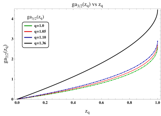
Figure 5: Characteristic curve of $ga_{3/2}(z_{q})$, $q$-generalized Bose integral of the first kind.

In Fig. 6 we have shown the characteristics of $gb_{3/2}(z_{q})$ for different $q$. Here this is the $q$-generalized Bose integral of the second kind, given by

$$gb_{5/2}(z_{q})=\frac{1}{\Gamma(5/2)}\int_{0}^{\infty}\frac{dx~{}x^{5/2-1}}{z_{q}^{-1}\left(e_{q}^{-x}\right)^{-q}-\left(e_{q}^{-x}\right)^{1-q}}$$ (65)

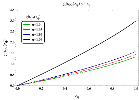
Figure 6: Characteristic curve of $gb_{5/2}(z_{q})$, $q$-generalized Bose integral of the second kind.

Interestingly both the functions in $q\rightarrow 1$ limit i.e., Eqs. (64) and (65) become our known Bose integrals which are as follows

$$g_{3/2}(z)=\frac{1}{\Gamma(3/2)}\int_{0}^{\infty}\frac{dx~{}x^{3/2-1}}{\left(ze^{-x}\right)^{-1}-1}$$ (66)

and

$$g_{5/2}(z)=\frac{1}{\Gamma(5/2)}\int_{0}^{\infty}\frac{dx~{}x^{5/2-1}}{z^{-1}e^{x}-1}$$ (67)

For $z_{q}=1$ these functions become Riemann-Zeta functions. In general for any $q$, Eq. (64) is equivalent to the $q$-generalized version of the Bose integrals given in [57, 58]. The plot obtained for the critical temperature $T_{c}$ as a function of the deformation parameter $q$ using our $q$-modified version of the polylog function of first kind and the same plot using the $q$-generalized version of the Bose integral given by [57, 58], are overlapping with each other(that is why we could not show the prediction of Ou et al.and Chen et al.in Fig. 1 separately [57, 58] with our prediction). The only difference is that, Ou et al.and Chen et al.used the same $q$-generalized version of the Bose integral as well to calculate the specific heat, whereas we used $q$-generalized Bose integral of the second kind to calculate the same. That is why our specific heat characteristics are little bit different from their prediction.

It is very difficult to derive an exact expression for the $q$-generalized mean occupation numbers from a more fundamental statistical description of a Bose gas which is strictly derived from more basic assumptions. Though we attempted to solve this issue using some algebraic assumptions which are reasonably valid under very restrictive conditions, an alternative strategy has been followed by Ou et al.and Chen et al.[57, 58]. They assumed a reasonably well defined $q$-generalized expression for the occupation number which is compatible with the general structures of the $q$-thermostatistical formalism. They investigated thoroughly and found that it exhibits physically appealing properties. Most importantly, though that expression cannot be obtained from the first principle at the moment, it agrees with the experimental result. Clearly the sensible choice of such an expression can correctly describe the experimental data.

References

- [1] Tsallis C 2009 Introduction to Nonextensive Statistical Mechanics: Approaching a complex World(Springer).
- [2] Nonextensive Statistical Mechanics and Its Applications, Sumiyoshi Abe Yuko Okamoto, (Lecture notes in physics ; Vol. 560), (Physics and astronomy online library), (Springer).
- [3] The standard map: From Boltzmann-Gibbs statistics to Tsallis statistics, Ugur Tirnakli and Ernesto P. Borges, Nature, Scientific Reports 6, Article number: 23644 (2016).
- [4] Nonextensive statistical mechanics - Applications to nuclear and high energy physics, Constantino Tsallis and Ernesto P. Borges, (February 2, 2008) [arXiv:cond-mat/0301521v1 [cond-mat.stat-mech]].
- [5] PRAMANA Indian Academy of Sciences Vol. 64, No. 5— journal of May 2005,physics, pp. 635–643, Boltzmann and Einstein: Statistics and dynamics –An unsolved problem, E G D COHEN.
- [6] Brazilian Journal of Physics, vol. 29, no. 1, March, 1999, Nonextensive Statistics:Theoretical, Experimental and Computational, Evidences and Connections, Constantino Tsallis (1998).
- [7] Some Comments on Boltzmann-Gibbs Statistical Mechanics, Constantino Tsallis, Pergamon, Chaos, Solitons & Fractals Vol. 6, pp. 539-559, 1995, Elsevier Science Ltd.
- [8] Non-extensive thermostatistics:brief review and comments, Constantino Tsallis, ELSEVIER Physica A 221 (1995) 277-290.
- [9] Generalized entropy as a measure of quantum uncertainty, M. Portesi, A. Plastino, ELSEVIER Physica A 225 (1996) 412-430.
- [10] Tsallis nonextensive thermostatistics, Pauli principle and the structure of the Fermi surface, F. Pennini, A. Plastino, A.R. Plastino, ELSEVIER Physica A 234 (1996) 471-479.
- [11] Generalized distribution functions and an alternative approach to generalized Planck radiation law, Ugur Tlrnakh, Fevzi Buyukkilic, Dogan Demirhan, ELSEVIER Physica A 240 (1997) 657-664.
- [12] Tsallis entropy and quanta1 distribution functions, F. Pennini, A. Plastino, A.R. Plastino, ELSEVIER Physics Letters A 208 (1995) 309-314.
- [13] Fevzi Buyukkilic, Phys. Lett. A 197 (1995) 2091.
- [14] G. Wilk, Z. Wlodarczyk, Phys. Rev. Lett. 84 (2000) 2770.
- [15] A. K. Rajagopal, S. Abe, Phys. Rev. Lett. 83 (1999) 1711.
- [16] R. Salazar, R. Toral, Phys. Rev. Lett. 83 (1999) 4233.
- [17] M.L.D. Ion, D.B. Ion, Phys. Rev. Lett. 83 (1999) 463.
- [18] M. Buiatti, P. Grigolini, A. Montagnini, Phys. Rev. Lett. 82 (1999) 3383.
- [19] D. Prato, Phys. Lett. A 203 (1995) 165.
- [20] Q.A. Wang, A.L. Mehaute, Phys. Lett. A 235 (1997) 222.
- [21] C. Tsallis, S.V.F. Levy, A.M.C. Souza, R. Maynard, Phys. Rev. Lett. 75 (1995) 3589.
- [22] B.M. Boghosian, Phys. Rev. E 53 (1996) 4754.
- [23] A.R. Plastino, A. Plastino, Phys. Lett. A 174 (1993) 384.
- [24] V.H. Hamity, D.E. Barraco, Phys. Rev. Lett. 76 (1996) 4664.
- [25] Asymptotics of superstatistics, Hugo Touchette, Christian Beck, Phys. Rev. E Stat Nonlin Soft Matter Phys. 2005 Jan;71(1 Pt 2):016131. Epub 2005 Jan 24; [arXiv:cond-mat/0408091v2] [cond-mat.stat-mech].
- [26] Recent developments in superstatistics, Christian Beck, Braz. J. Phys. vol.39 no.2a São Paulo Aug. 2009, [arXiv:0811.4363v2] [cond-mat.stat-mech].
- [27] Superstatistics: Recent developments and applications, Christian Beck, arXiv:cond-mat/0502306v1 [cond-mat.stat-mech].
- [28] Application to cosmic ray energy spectra and annihilation, C. Beck, Eur. Phys. J. A 40, 267–273 (2009) The European Physical Journal A, DOI 10.1140/epja/i2009-10792-7, Regular Article – Theoretical Physics, Superstatistics in high-energy physics.
- [29] Applications to high energy physics, Constantino Tsallis, EPJ Web of Conferences, 05001 (2011), DOI: 10.1051/epjconf/20111305001, Owned by the authors, published by EDP Sciences, 2011, Nonextensive statistical mechanics.
- [30] Generalization of the Planck radiation law and application to the cosmic wave background radiation, Constantino Tsallis, F. C. Sa Barreto, Edwin D. Loh, Phys. Rev. E, Vol. 52, No. 2 (1995).
- [31] M.L. Lyra, C.Tsallis, Phys. Rev. Lett. 80 (1998) 53.
- [32] P.A. Alemany, D.H. Zannette, Phys. Rev. E 49 (1994) 4754.
- [33] E.K. Lenzi, R.S. Mendes, Phys. Lett. A 250 (1998) 270.
- [34] A.R. Plastino, A. Plastino, Phys. Lett. A 193 (1994) 251.
- [35] A.R. Plastino, A. Plastino, H. Vucetich, Phys. Lett. A 207 (1995) 42.
- [36] D.F. Torres, H. Vucetich, A. Plastino, Phys. Rev. Lett. 79 (1997) 1588.
- [37] A.K. Rajagopal, Phys. Rev. Lett. 76 (1996) 3496.
- [38] G. Kaniadakis, A. Lavagno, P. Quarati, Phys. Rev. Lett. B 369 (1996) 308.
- [39] I. Koponen, Phys. Rev. E 55 (1997) 7759.
- [40] R.P. Di Sisto, S. Martinez, R.B. Orellana, A.R. Plastino, A. Plastino, Physica A 265 (1999) 590–613.
- [41] -deformed statistics and the role of light fermionic dark matter in SN1987A cooling, Atanu Guha, J. Selvaganapathy and Prasanta Kumar Das, Phys. Rev. D 95, 015001 (2017).
- [42] Blackbody radiation in -deformed statistics, Atanu Guha and Prasanta Kumar Das, arXiv:1706.10085.
- [43] -deformed Einstein’s Model to Describe Specific Heat of Solid, Atanu Guha and Prasanta Kumar Das, Physica A: Statistical Mechanics and its Applications 495C (2018) pp. 18-29.
- [44] The role of constraints within generalized nonextensive statistics, C. Tsallis, R. S. Mendes, A. R. Plastino, Physica A 261 (1998) 534.
- [45] Misusing the entropy maximization in the jungle of generalized entropies, T. Oikonomou, G.B. Bagci, Physics Letters A 381 (2017) 207.
- [46] Kamerlingh Onnes H., Proc. Roy. Acad. Amsterdam 13, 1903 (1911).
- [47] Keesom W.H. and Clausius K., Proc. Roy. Acad. Amsterdam 35, 307 (1932).
- [48] C. C. Bradley, C. A. Sackett, J. J. Tollett & R. G. Hulet (1995). ”Evidence of Bose–Einstein condensation in an atomic gas with attractive interactions”, Phys. Rev. Lett. 75 (9): 1687–1690. Bibcode:1995PhRvL..75.1687B. PMID 10060366. doi:10.1103/PhysRevLett.75.1687.
- [49] Dale G. Fried, Thomas C. Killian, Lorenz Willmann, David Landhuis, Stephen C. Moss, Daniel Kleppner & Thomas J. Greytak (1998). “Bose–Einstein Condensation of Atomic Hydrogen”. Phys. Rev. Lett. 81 (18): 3811. Bibcode:1998PhRvL..81.3811F. doi:10.1103/PhysRevLett.81.3811.
- [50] F. London (1938). “The λ-Phenomenon of liquid Helium and the Bose–Einstein degeneracy”. Nature. 141 (3571): 643–644. Bibcode:1938Natur.141..643L. doi:10.1038/141643a0.
- [51] “Bose–Einstein Condensation in Alkali Gases”, The Royal Swedish Academy of Sciences. 2001. Retrieved 17 April 2017.
- [52] R. K. Pathria and P. D. Beale, Statistical Mechanics, 3rd Ed. Academic Press (2011).
- [53] Generalized symmetric nonextensive thermostatistics and q-modified structures, A. Lavagno and P. Narayana Swamy, Mod. Phys. Lett. B 13, 961 (1999); arxiv:cond-mat/0001071v1[cond-mat.stat-mech] 7 Jan 2000.
- [54] Energy distribution and energy fluctuation in Tsallis statistics , Guo Ran, Du Jiulin, arXiv:1202.0638.
- [55] Daniel Vorberg, Waltraut Wustmann, Roland Ketzmerick, and Andre Eckardt, Phys. Rev. Lett. 111, 240405 (2013).
- [56] Sukanya Mitra, arXiv: 1709.02095 [nucl-th].
- [57] C. Ou and J. Chen, Phys. Rev. E 68, 026123 (2003).
- [58] J. Chen et al., Phys. Lett. A 300 (2002) 65-70.
- [59] W. H. Keesom and A. P. Keesom, Physica, Vol. 2, Issues 1-12, Pages 557-572 (1935).