A Novel Consensus-based Distributed Algorithm for Economic Dispatch Based on Local Estimation of Power Mismatch

Abstract

This paper proposes a novel consensus-based distributed control algorithm for solving the economic dispatch problem of distributed generators. A legacy central controller can be eliminated in order to avoid a single point of failure, relieve computational burden, maintain data privacy, and support plug-and-play functionalities. The optimal economic dispatch is achieved by allowing the iterative coordination of local agents (consumers and distributed generators). As coordination information, the local estimation of power mismatch is shared among distributed generators through communication networks and does not contain any private information, ultimately contributing to a fair electricity market. Additionally, the proposed distributed algorithm is particularly designed for easy implementation and configuration of a large number of agents in which the distributed decision making can be implemented in a simple proportional-integral (PI) or integral (I) controller. In MATLAB/Simulink simulation, the accuracy of the proposed distributed algorithm is demonstrated in a 29-node system in comparison with the centralized algorithm. Scalability and a fast convergence rate are also demonstrated in a 1400-node case study. Further, the experimental test demonstrates the practical performance of the proposed distributed algorithm using the VOLTTRON™ platform and a cluster of low-cost credit-card-size single-board PCs.

I Introduction

Future power systems are equipped with a great number of distributed generators (DGs), distributed energy storage devices, dispatchable loads and advanced communication networks, which increases the customer participation in the electricity market. As a result, the optimal economic dispatch (ED) of future power systems is becoming much more challenging. A sophisticated control is needed to fully address the increasing customer participation at the edge of the electric power system and the inability of existing practices to accommodate these changes [1, 2, 3, 4].

Figure 1: Different approaches for power grids. (a) centralized approach, (b) distributed approach (peer-to-peer connections)

In a centralized ED, all participants (DGs and consumers) must release their information to the central controller. As the market penetration of DGs and consumers is continuously growing, the centralized algorithms are no longer suitable due to the heavy computational burden [5]. Moreover, the centralized algorithms are not designed to support plug-and-play functionalities of a large number of participants.

Consensus-based distributed approaches have been found to be practical in many multi-agent applications, such as industrial systems, automated high way systems, and computer networks [6]. Consensus-based distributed approaches are to find the global optimal decision by allowing local agents to iteratively share information through two-way communication links. All agents reach a consensus when they agree upon the value of the information state [7, 8, 9, 10, 11]. The information state can be physical quantities or control signals such as voltage, frequency, output power, incremental cost, and estimated power mismatches [12]. Figure 1 compares the centralized and distributed methods for solving the ED problem in power systems [13]. The major advantages of distributed methods are summarized as follows:

Scalability and Interoperability: As the number of agents increases to hundreds of thousands, the legacy centralized method faces certain challenges such as computational burden. As more DGs are integrated into power systems, the centralized methods are not suitable for such heterogeneous systems [12, 14].

Monopoly and Monopsony: A central organization usually has a kind of monopoly over the consumers and a monopsony toward the electrical energy DGs. However, as it is discussed in various research papers and academic notes, consumers have a much more apathetic role than DGs do in electrical energy markets under centralized control [15, 16].

Privacy and Stealth Protection: One of the essential and notable features of every competitive system is the equal opportunity for competition for all players. Therefore, it should be ensured that no private information is released by a third-party and no preferences are given to one or more DGs in a competitive market [1].

Computational Cost: Heavy computational load is imposed on the central controller when dealing with a large multi-agent network [12, 17]. However, the computational load can be shared among agents using distributed approaches.

Single Point of Failure: A distributed approach is robust to the single point of failure because there is no need for a center for the supervisory of the entire system [14, 18].

Network Topology: In future power systems, the communication network and power network are subject to frequent change [19]. Accordingly, there are serious doubts about the ability of centralized methods to handle the variable topology.

The literature review shows a growing interest in distributed algorithms in the field of power systems. A distributed algorithm for solving the ED problem that considered thermal generation and random wind power was discussed in [20] for a smart grid. A distributed optimization problem with local constraints was studied in [21] to obtain the optimal solution for a load sharing problem. Hug and Kar [22] introduced a consensus-based distributed energy management approach to handle loads of a micro-grid. Rahbari-Asr et al. investigated an incremental welfare consensus-based algorithm that manages both loads and DGs [23]. In addition, they developed a cooperative distributed demand management system in [24] based on Karush–Kuhn–Tucker conditions for plug-in electric vehicle charging. A distributed optimal power flow was introduced for a large-size distribution system in [25]. Mudumbai et al. [5] worked on the distributed algorithm for both optimal ED and frequency control with a large number of intermittent energy sources. The authors in [26] proposed a distributed real-time demand response for a multi-agents system to maximize social welfare. They defined sub-problems by decomposing the main optimization problem and locally solving each sub-problem. Binetti et al. [9] presented a distributed method to solve the ED problem considering power losses of transmission lines. Two consensus protocols were run in parallel to reach the consensus and estimate the power-mismatch considering the lines’ losses. Elsayed and El-Saadany proposed a fully decentralized method that can solve both the convex and the practical non-convex ED problem. They also considered transmission losses in [27]. In [28], a distributed constrained gradient approach was proposed to consider both the equality and inequality constraints for online optimal generation control. Another algorithm has been introduced in [29] to help energy producers to collect information regarding power mismatch between generation and consumption. This mechanism finally converges incremental cost to an optimal value. N. Cai et al. [30] offers a decentralized approach for the economic dispatch problem of a micro-grid in which, various agents use local information or receive some information from their immediate neighbors. However, this paper does not cover the power balance within micro-grid because it is assumed that power balance has already been met. One of the distributed techniques for solving non-convex economic dispatch problem has been introduced in [31]. In this technique, a leader-less consensus based distributed algorithm share bids among different agents based on an auction mechanism. G. Binetti et al. considered transmission losses, valve-point loading effect, multiple fuel, prohibited operating zones in non-convex ED problem. A primal-dual perturbation method is proposed by T.H Chang et al. [32] enabling multi-agents system to reach a global optimum. In this method, all agents try to estimate functions of global cost and constraints based on distributed approach.

From the control algorithm’s point of view, one common issue with existing distributed consensus algorithms is their slow convergence (high iteration numbers), privacy, high connectivity requirement and complexity. For instance, in most of previous works the incremental cost ($\lambda$) and output power are shared [26], which violate privacy principles. While agents in a multi-agent system may not share private information with center (third-party), they share the private information with other agents and it could be even worse than the centralized method. In addition, distributed methods cannot attract serious attentions in case of implementation if they suffer from high connectivity, slow convergence and complexity. To address the aforementioned limitations of existing distributed methods, we propose a novel consensus-based distributed algorithm to maintain data privacy and reduce computational time while solving for a large-scale ED problem. The proposed approach need to share minimum information (Power mismatch) among different agents in a multi-agent network, thus, the privacy of all agents will definitely be improved. In other words, the parameter of cost function, utility function, incremental cost ($\lambda$) and output power etc. will not be shared among agents and, also, third-party are not at all able to access to these parameters. In addition, computational cost will be decreased that make the scalability possible for enormous multi-agent system. Figure 2 shows a general view of the communication network for the proposed method. The main features of the proposed distributed algorithm are as follows:

1. Accuracy: The ED problem is solved in a fully distributed manner without relying on a central controller. The solution accuracy is validated by the benchmark results achieved by traditional centralized methods.

2. Privacy: DGs and consumers do not need to disclose any private information (e.g., cost functions and utility functions) with others. The estimated power mismatch between the total generation and the total demand is the only information to be shared among all DGs. In addition, consumers are not required to have a communication channel between one another or to exchange information with all DGs. They only need to connect to local DGs.

3. Fast Convergence: The proposed algorithm outperforms some existing distributed methods in terms of number of iteration and computational time.

4. Scalability: The proposed distributed algorithm is particularly suitable for solving large-scale optimization problems (e.g., ¿1,000 agents) within a short period of time.

5. Easy Implementation: This salient feature makes it possible to deploy the proposed distributed methods in the field at scale.

Figure 2: The illustrated communication network for the proposed distributed method.

The structure for the rest of this paper is organized as follows: Section II formulates the ED problem as a global objective function, considering cost functions, utility functions and constraints. Section III discusses graph theory, consensus-based distributed protocols, optimality and convergence analysis of proposed algorithm . Section IV evaluates the solution performance using software simulation and experimental testing. Section V summarizes this paper and presents the concluding remarks.

II System Modeling and Problem Description

The ED problem is a short-term resource allocation of a number of DGs to meet the load requirement in a most cost-effective way. The utility function of consumers, the cost function of DGs and their surplus function are defined in this section. Then, the overall optimization problem is formulated based on the defined model of economic players in an electricity market.

II-A Utility Function, Marginal Benefit and Consumer’s Surplus

Each consumer in an electricity market has its own preferences for energy consumption during different times of a day. These preferences cause various levels of requested demand within an operation period. There are some factors affecting the preferences of consumers in an electricity market such as the instantaneous or average price of electricity, temperature changes, the type of user and comfort level. The different demand levels requested by consumers in response to these diverse factors can be modeled by utility functions for mathematical purposes [16, 26, 33]. In other words, the utility function measures the satisfaction level or welfare of consumers as a function of different types of performance (i.e., demand level) to represent a consumer’s preferences. In a typical electricity market, the utility function $U_{j}(P_{j}^{Load})$ shows the level of satisfaction of the $j-th$ energy consumer, where $P_{j}^{Load}$ is the demand of $j-th$ consumer.

Marginal benefit is an additional utility that an electrical consumer will gain by getting one more unit ($\mathrm{MW}$) of electrical energy. The consumption of more power increases the utility function if the marginal benefit has a positive value; however; the consumption of more power decreases the level of satisfaction if the marginal benefit has a negative value [34]. The common utility functions are non-decreasing functions; thus, the marginal benefit is a non-negative function. It means [35, 36]:

$$\frac{\partial U_{j}\left(P_{j}^{Load}\right)}{\partial P_{j}^{Load}}\geq 0,\qquad j\epsilon S_{D}$$ (1)

It is evidently proven that the marginal benefit of electrical consumers is a non-increasing function because the marginal benefit will normally decrease as users consume more energy. Thus, we have [35, 36]:

$$\frac{\partial^{2}U_{j}\left(P_{j}^{Load}\right)}{\partial\left(P_{j}^{Load}\right)^{2}}\leq 0,\qquad j\epsilon S_{D}$$ (2)

There are various types of utility function for single and multiple goods, such as: Cobb-Douglas Utility Function, Perfect Substitutes, Perfect Complements and Quasilinear [37]. In this paper, a quadratic mathematical model satisfying (1) and (2) is used in Equation (3) as a utility function of the consumers. This utility function is customized for different consumers based on parameters $b\,\nicefrac{\mathrm{\$}}{\mathrm{kWh^{2}}}$ and $\omega\,\nicefrac{\mathrm{\$}}{\mathrm{kWh}}$. The larger $\omega$ is, the higher the utility function [26].

$$U_{j}\left(P_{j}^{Load}\right)=\begin{cases}\omega_{j}P_{j}^{Load}-b_{j}(P_{j}^{Load})^{2}&P_{j}^{Load}\leq\nicefrac{{\omega_{j}}}{{2b_{j}}}\\ \frac{\omega_{j}^{2}}{4b_{j}}&P_{j}^{Load}\geq\nicefrac{{\omega_{j}}}{{2b_{j}}}\end{cases}$$ (3)

Consumer’s surplus measures the welfare on the consumers’ side; hence, it is a measurement of the benefit, derived from the electricity market, of an economic player on the consumption side [23]. A consumer’s surplus will be represented by (4), if the $j-th$ consumer pays $\lambda\;\nicefrac{\mathrm{\$}}{\mathrm{kWh}}$ for $P_{j}^{Load}\;\mathrm{kW}$ of the electrical energy.

$$\mathcal{S}_{j}^{Load}\left(P_{j}^{Load}\right)=U_{j}\left(P_{j}^{Load}\right)-\lambda P_{j}^{Load},\qquad j\epsilon S_{D}$$ (4)

Consumers attempt to maximize their own welfare in the market. Therefore, they consume power at the maximum value of their concave surplus function. Figure 3 shows the graphical representation of equations (3) and (4).

Figure 3: Consumer’s surplus and utility function

II-B Cost Function and DG’s Surplus

Generally speaking, a multiple piecewise linear or quadratic function, known as cost function, is used to estimate the total cost of the output-power of the energy providers, such as DGs. Using a proper cost function is the best way to pre-evaluate the performance of a DG and to solve an ED problem [15, 33]. Here, we consider a quadratic mathematical equation to model a typical DG. $\alpha\,\nicefrac{\mathrm{\$}}{\mathrm{kWh^{2}}}$, $\beta\,\nicefrac{\mathrm{\$}}{\mathrm{kWh}}$ and $\gamma\,\nicefrac{\mathrm{\$}}{\mathrm{h}}$ are coefficients that customize the cost function for each DG and $P_{i}^{Gen}$ is power generated by the $i-th$ DG.

$$C_{i}\left(P_{i}^{Gen}\right)=\alpha_{i}(P_{i}^{Gen})^{2}+\beta_{i}P_{i}^{Gen}+\gamma_{i},\qquad i\epsilon S_{G}$$ (5)

A DG’s surplus (commonly known as profit) measures the welfare of a DG. In other words, it is a benefit gained by DG, when the sale price of energy is more than the costs spent to produce the energy. If the $i-th$ DG sells $P\,\mathrm{kW}$ of electrical energy at $\lambda\;\nicefrac{\mathrm{\$}}{\mathrm{kWh}}$, the DG’s profit is expressed as in (6).

$$\mathcal{S}_{i}^{Gen}\left(P_{i}^{Gen}\right)=\lambda P_{i}^{Gen}-C_{i}\left(P_{i}^{Gen}\right),\qquad i\epsilon S_{G}$$ (6)

Unlike consumers, DGs tend to produce as much electricity as possible. Figure 4 shows the surplus curve of a DG. The more power DGs produce, the higher surplus they obtain.

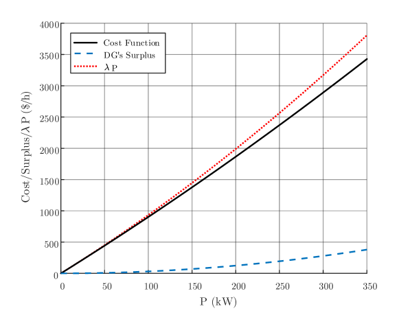
Figure 4: A DG’s surplus and cost function

II-C Global Optimization Problem

The objective function in this paper is to maximize the welfare of all consumers and DGs. In other words, the objective function is to maximize the summation of the utility functions (3) and minimize the summation of the cost functions (5). Thus, the overall objective function can be written as:

$$Min\left(\underset{i\epsilon S_{G}}{\sum}C_{i}\left(P_{i}^{Gen}\right)-\underset{j\epsilon S_{D}}{\sum}U_{j}\left(P_{j}^{Load}\right)\right)$$ (7)

Note that the current version of the proposed distributed algorithm does not consider the power losses and the maximum capacity of the power lines. This objective function is also subject to constraints of power balance between the aggregated generations ($\underset{i\epsilon S_{G}}{\sum}P_{i}^{Gen}$ ) and consumption ($\underset{j\epsilon S_{D}}{\sum}P_{j}^{Load}$ ) as in (8).

$$\underset{i\epsilon S_{G}}{\sum}P_{i}^{Gen}=\underset{j\epsilon S_{D}}{\sum}P_{j}^{Load}$$ (8)

In addition, the output-power of each DG and the consumption of each consumer cannot go beyond their maximum capacity. These two constraints can be applied to the optimization problem as in (9).

$$0\leq P_{i}^{Gen}\leq P_{i,max}^{Gen}\qquad i\epsilon S_{G}$$

$$0\leq P_{j}^{Load}\leq P_{j,max}^{Load}\qquad j\epsilon S_{D}$$ (9)

III Distributed Algorithm for Economic Dispatch

As previously mentioned, consensus-based distributed approaches offer a great solution for solving optimization problems such as economic dispatch. In this section, we review the conception of the graph theory and elaborate on the proposed distributed algorithm in details.

III-A Graph Theory

We can model the agents’ interaction through the communication network by (un)directed graphs denoted by $\mathcal{G}(\mathcal{V},\xi)$. Consider a network of $n$ connected agents in which nodes are designated by $\mathcal{V}=\{v_{1},v_{2},\ldots v_{p}\}$ and $\xi\subseteq\mathcal{V}\times\mathcal{V}$ shows a set of edge. The directed edge $\vec{e_{ij}}=(v_{i},v_{j})$ shows that agent $i$ share it’s information state with agent $j$. Also, undirected edge $e_{ij}=(v_{i},v_{j})$ indicates that agents $i$ and $j$ can share information with each other. Two matrices will commonly be used to represent the communication topology of a multiple-agents network. The adjacency matrix denoted by $\mathcal{A}=\{\left[a_{ij}\right]|a_{ij}\in\mathcal{R^{P\times P}}\}$ of an undirected graph $\mathcal{G}$ is symmetric. The entry $a_{ij}$ of an adjacency matrix is a positive value if $e_{ij}\in\xi$ and $a_{ij}=0$ for $e_{ij}\notin\xi$. Otherwise, the entry $a_{ii}$ is assumed to be zero. The second matrix is Laplacian matrix $L=\{\left[l_{ij}\right]|l_{ij}\in\mathcal{R^{P\times P}}\}$ in which entry $l_{ii}=\underset{j\quad}{\sum a_{ij}}$ and $l_{ij}=-a_{ij}$ for $i\neq j$ . Equation (10) shows matrices $\mathcal{A}$ and $L$ [18, 20, 6].

$$A=\left[\begin{array}[]{cccc}a_{11}&a_{12}&\cdots&a_{1n}\\ a_{21}&a_{22}&\cdots&a_{2n}\\ \vdots&\vdots&\ddots&\vdots\\ a_{n1}&a_{n2}&\cdots&a_{nn}\end{array}\right]\\ L=\left[\begin{array}[]{cccc}\underset{j\quad}{\sum a_{1j}}&-a_{12}&\cdots&-a_{1n}\\ -a_{21}&\underset{j\quad}{\sum a_{2j}}&\cdots&-a_{2n}\\ \vdots&\vdots&\ddots&\vdots\\ -a_{n1}&-a_{n2}&\cdots&\underset{j\quad}{\sum a_{nj}}\end{array}\right]\qquad\qquad\quad\;\;$$ (10)

III-B Consensus-based Distributed Protocols

In consensus-based distributed approaches, a network of agents shares information via communication channels between agents to reach a consensus. Node $i$ and node $j$ have reached a consensus if and only if the value of the state of the $i-th$ node ($x_{i}$) and the state of the $j-th$ node ($x_{j}$) are equal [8, 6]. Thus, multiple agents reach a consensus when all of them agree on the coordination information or variable. The Laplacian potential for a graph is delineated by (11) which represents a kind of virtual energy stored in a graph [38].

$$\mathcal{L_{P}=}\underset{i,j}{\sum}a_{ij}(x_{j}-x_{i})^{2}=2x^{T}Lx$$ (11)

In other words, the Laplacian potential could be used as a measure that shows the total disagreement among all agents in a network. If the agents of a network tend to reach a consensus, they should at least interact with their neighbors to minimize Laplacian potential ($\mathcal{L_{P}}$) as a disagreement [6]. In fact, a general consensus for a multi-agent system will be reached if and only if $\mathcal{L_{P}}=0$ or $x_{i}=x_{j}$.

The “consensus” being used for the proposed method is defined as zero-power-mismatch. Based on the definition of Laplacian potential, the whole power mismatch is a virtual energy stored in the network that must be minimized. Consensus is reached by converging towards

$$\varDelta P_{1}^{T}=\varDelta P_{2}^{T}=\cdots=\varDelta P_{n}^{T}=0$$ (12)

where $\varDelta P_{i}^{T}$ is a power mismatch of the whole system estimated by the $i-th$ DG.

Considering that all agents have single-integrator dynamics [6, 38], a standard linear consensus protocol is defined as (13).

$$\dot{x_{i}}(t)=\underset{j}{\sum}a_{ij}(x_{j}-x_{i})$$ (13)

Equation (13) can be written for all agents as a vector: $\dot{x}(t)=-Lx$, which is equivalent to the gradient of the Laplacian potential of a graph as shown in Equation (14). It represents a gradient-descent algorithm that is able to find the minimum of the Laplacian potential function. As previously discussed, the minimum Laplacian potential happens at $\varDelta P_{i}=0,\quad\;\forall i$.

$$\dot{x_{i}}(t)=-\nabla\mathcal{L_{P}}$$ (14)

A discrete-time version of the linear consensus protocol of a first-order integrator can be represented by (15)

$$x_{i}(k+1)-x(k)=u_{i}(k)\Longrightarrow$$

$$x_{i}(k+1)=x_{i}(k)+u_{i}(k)\quad\quad$$ (15)

where $u_{i}(k)$ depends on the information state of neighbors of $i-th$ agent (i.e., $u_{i}=f_{i}(x_{1},x_{2},...,x_{j})$) and can be shown by (16).

$$u_{i}(k)=\underset{j}{\sum}a_{ij}(x_{j}(k)-x_{i}(k))$$ (16)

Equation (17) is obtained from (15) and (16), where $I$ is unit matrix.

$$x_{i}(k+1)=x_{i}(k)+\underset{j}{\sum}a_{ij}(x_{j}(k)-x_{i}(k))\Longrightarrow$$

$$x_{i}(k+1)=x_{i}(k)-Lx_{i}(k)=(I-L)x_{i}(k)$$ (17)

Given that the sum of row of adjacency matrix A is one (i.e., A is a stochastic matrix), Equation (18) can be derived from (17). Equation (18) explicitly indicates that the next state of each agent depends on the current states of other agents.

$$x_{i}(k+1) =\underset{j}{\sum}a_{ij}x_{j}(k)$$ (18)

Now, we consider $\varDelta P$ as information coordination that needs to be shared among agents. Equation (19) shows that $\varDelta P$ of each agent is calculated by the current estimated $\varDelta P$ of other neighbors. It is worth mentioning that $\varDelta P$, the only information shared among different agents, does not include any private information. The consumers do not need to launch any communication link among themselves for information coordination. Thus, the elements associated with the connectivity between any pair of consumers are zero in “Matrix A”. Moreover, consumers do not have to establish a communication channel with more than one DG. They are connected to a local or nearest DG if there is a physical connection (transmission and distribution line). Since the power mismatch is the only shared information among DGs, a DG and its associated loads/consumers can be viewed as an aggregate node. The “Reduced Matrix A” being used in Equation (19) is only an adjacency matrix of DGs’ communication network. In sum, the A matrix has many zero elements that most of them could be ignored for the sake of simplicity. The A matrix that used in Equation (19) is only an adjacency matrix of DGs’ communication network without zero elements of consumers’ network and communication channel among consumers and DGs. Thus, we omitted zero elements. The A matrix is reduced by dimension in comparison with A matrix of the entire system.

$$\left[\begin{array}[]{c}\varDelta P_{1}\left(k+1\right)\\ \varDelta P_{2}\left(k+1\right)\\ .\\ .\\ .\\ \varDelta P_{n}\left(k+1\right)\end{array}\right]=\left[A\right]\left[\begin{array}[]{c}\varDelta P_{1}\left(k\right)\\ \varDelta P_{2}\left(k\right)\\ .\\ .\\ .\\ \varDelta P_{n}\left(k\right)\end{array}\right]\\ \\ \Longrightarrow\vec{\varDelta P}\left(k+1\right)=A\vec{\varDelta P}\left(k\right)\quad\quad\quad\quad\quad\quad\quad$$ (19)

Each DG uses its own estimated power mismatch as a feedback. By adding the vector $\vec{P}^{L}(k)-\vec{P}^{Gen}\left(k\right)$ to Equation (19), Equation (LABEL:eq:completedeltaP) is obtained as a consensus protocol for this paper.

$$\vec{\varDelta P^{T}}\left(k+1\right)=A\vec{\varDelta P}\left(k\right)+\vec{P}^{L}\left(k\right)-\vec{P}^{Gen}\left(k\right)$$

$$\Longrightarrow\left[\begin{array}[]{c}\varDelta P_{1}^{T}\left(k+1\right)\\ \varDelta P_{2}^{T}\left(k+1\right)\\ .\\ .\\ .\\ \varDelta P_{n}^{T}\left(k+1\right)\end{array}\right]=\left[A\right]\left[\begin{array}[]{c}\varDelta P_{1}\left(k\right)\\ \varDelta P_{2}\left(k\right)\\ .\\ .\\ .\\ \varDelta P_{n}\left(k\right)\end{array}\right]+$$ (32)

$$\left[\begin{array}[]{c}P_{1}^{L}\left(k\right)-P_{1}^{Gen}\left(k\right)\\ P_{2}^{L}\left(k\right)-P_{2}^{Gen}\left(k\right)\\ .\\ .\\ .\\ P_{n}^{L}\left(k\right)-P_{n}^{Gen}\left(k\right)\end{array}\right]\qquad$$ (39)

Where $P_{i}^{L}$ is the summation of all local loads connected to $i-th$ DGs. Every iteration, the DGs need to go through a simple process to update incremental cost $\lambda$ internally. This $\lambda$ does not need to be shared with neighbors. Once gain, the only information that will be shared through the communication network is $\varDelta P$.

The discrete-time equation (41) shows proposed protocol for $\lambda$ in this paper, where $\varDelta x>0$ shows the interval of discrete-time integration, and $K_{I}$ is the controller coefficient.

$$\lambda_{i}\left(k+1\right)=K_{I}\underset{k}{\sum}\left(\varDelta P_{i}^{T}\left(k+1\right)+\varDelta P_{i}^{T}\left(k\right)\right)\times\frac{\varDelta x}{2}$$ (41)

The incremental cost $\lambda$ is used to calculate output-power ($P_{i}^{Gen}$) of a DG, The parameters of cost function (5) such as $\alpha$, $\beta$ and the calculated $\lambda$ inside the controller of each agent are used to estimate output-power using Equation (42). In fact, other agents and third-parties are not at all able to access these parameters.

$$P_{i}^{Gen}\left(k+1\right)=\begin{cases}0&P_{i}^{Gen}\leq 0\\ \frac{\lambda_{i}\left(k+1\right)-\beta_{i}}{2\alpha_{i}}&0<P_{i}^{Gen}<P_{i,max}^{Gen}\\ P_{i,max}^{Gen}&P_{i}^{Gen}\geq P_{i,max}^{Gen}\end{cases},$$

$$\qquad i\epsilon S_{G}$$ (42)

When a DG estimates its output-power, it can determine the estimated power mismatch by Equation (43), and share this estimate with its neighbors at each iteration.

$$\varDelta P_{i}\left(k+1\right)=P_{i}^{Gen}\left(k+1\right)-P_{j}^{L}(k+1),\qquad i\epsilon S_{G}$$ (43)

When a DG determines its $\lambda$ in accordance with its output-power, it shares $\lambda$ with the local consumers. Then the consumers calculate their demands based on the $\lambda$ offered by the DG. It is not, however, necessary to share $\lambda$ among consumers; in other words, each consumer just needs to receive $\lambda$ from one DG. Then, the consumer can determine its best and most cost-effective demand based on the maximum level of the consumer’s surplus function represented by (4). The maximum of consumer’s surplus can be achieved by $\frac{\partial\mathcal{S}_{j}^{Load}}{\partial P_{j}^{Load}}=0$, which is shown in (44). The utility function of consumers in Equation (3) and Figure 3 show that if a consumer uses power more than $\nicefrac{{\omega_{j}}}{{2b_{j}}}$ , its level of satisfaction will not be increased. Thus, the maximum load of $j-th$ consumer is considered as $P_{j,max}^{Load}=\nicefrac{{\omega_{j}}}{{2b_{j}}}$.

$$P_{j}^{Load}(k+1)=\begin{cases}0&P_{j}^{Load}\leq 0\\ \frac{\omega_{j}-\lambda_{i}\left(k+1\right)}{2b_{j}}&0<P_{j}^{Load}<P_{j,max}^{Load}\\ P_{j,max}^{Load}&P_{j}^{Load}\geq P_{j,max}^{Load}\end{cases},$$

$$\qquad j\epsilon S_{D}$$ (44)

The consumer sends the amount of estimated demand to a local DG if there is a physical connection (i.e., distribution lines) between them. The consumers do not need to disclose any properties of its utility function. In addition, consumers do not need to establish any communication channel among themselves to coordinate any information state or with more than one DG. The above-mentioned features significantly reduce the computing complexity and the upfront cost of new communication infrastructure

Figure 5 illustrates the interaction between a specific DG and other agents (DGs and consumers).

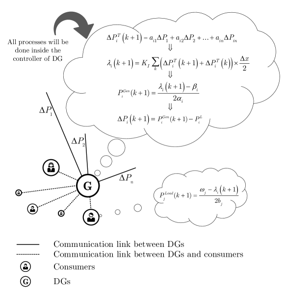
Figure 5: Distributed decision making for a DG at every iteration.

The optimality and convergence analysis of the proposed distributed algorithm will be discussed in the rest of this section.

III-C The Optimality Analysis

As mentioned before, $P_{i}^{L}$ is the summation of local loads connected to $i-th$ DG. Equation (45) shows the $\left(k+1\right)-th$ iteration of total $P_{i}^{L}$ and $\psi_{i}$ indicates the portion of total load connected to $i-th$ DG. $\theta_{i}^{L}$ and $\varphi_{i}^{L}$ are used in the place of $\psi_{i}\underset{j}{\sum}\frac{\omega_{j}}{2b_{j}}$ and $\psi_{i}\underset{j}{\sum}\frac{1}{2b_{j}}$ , respectively, for more simplicity. $\left(k+1\right)-th$ iteration of DG’s output is calculated by (46). In addition, $\theta_{i}^{Gen}$ and $\varphi_{i}^{Gen}$ are used in the place of $\frac{\beta_{i}}{2\alpha_{i}}$ and $\frac{1}{2\alpha_{i}}$, respectively.

$$P_{i}^{L}(k+1)=\psi_{i}\underset{j}{\sum}P_{j}^{Load}(k+1)$$

$$=\psi_{i}\underset{j}{\sum}\frac{\omega_{j}}{2b_{j}}-\psi_{i}\underset{j}{\sum}\frac{1}{2b_{j}}*\lambda_{i}(k+1)$$

$$=\theta_{i}^{L}-\varphi_{i}^{L}\lambda_{i}(k+1);\quad\underset{j}{\sum}\psi_{i}=1$$ (45)

$$P_{i}^{Gen}(k+1)=\frac{\lambda_{i}(k+1)-\beta_{i}}{2\alpha_{i}}=\frac{\lambda_{i}(k+1)}{2\alpha_{i}}-\frac{\beta_{i}}{2\alpha_{i}}$$

$$=\varphi_{i}^{Gen}\lambda_{i}(k+1)-\theta_{i}^{Gen}$$ (46)

Finally, the power mismatch $\Delta P_{i}(k+1)$ calculated by $i-th$ DG is achieved by (47) where, $\varphi_{i}^{c}=\varphi_{i}^{Gen}+\varphi_{i}^{L}$ and $\theta_{i}^{c}=\theta_{i}^{Gen}+\theta_{i}^{L}$.

$$\Delta P_{i}(k+1)=P_{i}^{Gen}(k+1)-P_{i}^{L}(k+1)$$

$$=\left(\varphi_{i}^{Gen}+\varphi_{i}^{L}\right)\lambda_{i}(k+1)-\left(\theta_{i}^{Gen}+\theta_{i}^{L}\right)$$

$$=\varphi_{i}^{c}\lambda_{i}(k+1)-\theta_{i}^{c}$$ (47)

$\lambda_{i}$, $\Delta P_{i}^{T}$ of $i-th$ agent for $k=0$ can be calculated by (20), (23) and (25) .

$$\Delta P_{i}^{T}(1)=\Delta P_{1}(0)+\Delta P_{2}(0)+\cdots=\Delta_{1}$$ (48)

$$\Delta P_{i}^{T}(0)=\Delta P_{1}(0^{-})+\Delta P_{2}(0^{-})+\cdots=\Delta_{0}$$ (49)

$$\lambda_{i}(1)=K_{I}(\Delta P_{i}^{T}(1)+\Delta P_{i}^{T}(0))=K_{I}(\Delta_{1}+\Delta_{0})$$ (50)

By continuing this process for $k=1,\,2,\,\cdots$, equations (51), (52) will be obtained.

$$\Delta_{k+1}=\Delta P_{i}^{T}(k+1)=\underset{i}{\sum}K_{I}\varphi_{i}^{c}\Delta_{k}-\Delta_{k}\quad\forall i\epsilon S_{G}$$ (51)

$$\lambda_{i}(k+1)=K_{I}(\Delta_{k}+\cdots+2\Delta_{2}+2\Delta_{1}+\Delta_{0})\quad\forall i\epsilon S_{G}$$ (52)

In Equation (51), $||\Delta_{k+1}||$ merges to zero i.e.; $||\Delta_{k+1}||\rightarrow 0$ if $||\underset{i}{1-\sum}K_{I}\varphi_{i}^{c}||\leq\varepsilon<1$, where where $\varepsilon$ is a positive number. Then, we have $\lambda_{i}(k+1)\leq(\varepsilon^{k}\Delta_{0}+2\varepsilon^{k-1}\Delta_{0}\cdots+2\varepsilon^{2}\Delta_{0}+2\varepsilon\Delta_{0}+\Delta_{0}),\quad\forall i\epsilon S_{G}$. Therefore, if $k\rightarrow\infty$, $\lambda_{i}$will not approach infinity; hence, $\lambda_{i}(k+1)\leq\frac{1}{1-\varepsilon}\Delta_{0}+\frac{\varepsilon}{1-\varepsilon}\Delta_{0}=\frac{1+\varepsilon}{1-\varepsilon}\Delta_{0}$. The smaller $||\underset{i}{1-\sum}K_{I}\varphi_{i}^{c}||$ is, the faster the power mismatch will converge to $0$. $K_{I}$ is the parameter that can control/change the size of $||\underset{i}{1-\sum}K_{I}\varphi_{i}^{c}||$ to be less than $1$.

Finally, Equation (53) indicates that $\lambda_{i}$ for all DG ($\forall i$) will be same and $\Delta P_{i}^{T}(k+1)$ of $i-th$ of DG will converge to zero for $\forall i\epsilon S_{G}$. We consider all $\lambda_{i}\quad\forall i$ as $\lambda$ because they are identical. In the next step, we will show (53) will satisfy the KKT conditions.

$$\underset{k\rightarrow\infty}{lim}\;\lambda_{i}(k+1)=\lambda;\qquad\forall i\epsilon S_{G}$$

$$\underset{k\rightarrow\infty}{lim}\;\Delta P_{i}^{T}(k+1)=\Delta_{k+1}=0;\qquad\forall i\epsilon S_{G}$$ (53)

Assumption 1: All local cost functions utility functions (3) and (5) are strictly concave and convex, respectively. Accordingly, the total objective function (7) is strictly convex.

Assumption 2: In addition, all equality and inequality constraint functions, represented by (8) and (9), are affine.

Lemma 1: The optimization problem represented in this paper through (3)-(9) is a convex optimization problem with differentiable objective and constraint functions satisfying Slater’s condition (assumption 1 and 2 guarantee Slater’s condition), thus the KKT conditions provide necessary and sufficient conditions for optimality [39].

The remaining of this section makes certain that the fixed-point of proposed iterative consensus algorithm obtained by (LABEL:eq:completedeltaP)-(44) is a global optimal solution of (7) if it is satisfying the following KKT conditions [21].

Lagrangian:

$$L(P,\lambda,\mu,\zeta)=\left(\underset{i\epsilon S_{G}}{\sum}C_{i}\left(P_{i}^{Gen}\right)-\underset{j\epsilon S_{D}}{\sum}U_{j}\left(P_{j}^{Load}\right)\right)$$

$$+\lambda\left(\underset{j\epsilon S_{D}}{\sum}P_{j}^{Load}-\underset{i\epsilon S_{G}}{\sum}P_{i}^{Gen}\right)$$

$$+\underset{i\epsilon S_{G}}{\sum}\mu_{i}\left(P_{i}^{Gen}-P_{i,max}^{Gen}\right)+\underset{i\epsilon S_{G}}{\sum}\zeta_{i}\left(-P_{i}^{Gen}\right)$$

$$+\underset{j\epsilon S_{D}}{\sum}\mu_{j}\left(P_{j}^{Load}-P_{j,max}^{Load}\right)+\underset{j\epsilon S_{D}}{\sum}\zeta_{j}\left(-P_{j}^{Load}\right)$$ (54)

Lagrangian stationarity ($\nabla_{P}L(P,\lambda,\mu,\zeta)$=0):

$$\frac{\partial C_{i}\left(P_{i}^{Gen}\right)}{\partial\left(P_{i}^{Gen}\right)}-\lambda+\mu_{i}-\zeta_{i}=0;\qquad\forall i\epsilon S_{G}$$

$$-\frac{\partial U_{j}\left(P_{j}^{Load}\right)}{\partial\left(P_{j}^{Load}\right)}+\lambda+\mu_{j}-\zeta_{j}=0;\qquad\forall j\epsilon S_{D}$$ (55)

Complementary slackness:

$$\mu_{i}\left(P_{i}^{Gen}-P_{i,max}^{Gen}\right)=0\,,\quad\zeta_{i}\left(-P_{i}^{Gen}\right)=0;\qquad\forall i\epsilon S_{G}$$

$$\mu_{j}\left(P_{j}^{Load}-P_{j,max}^{Load}\right)=0\,,\quad\zeta_{j}\left(-P_{j}^{Load}\right)=0;\qquad\forall j\epsilon S_{D}$$ (56)

Dual feasibility:

$$\mu_{i}\geq 0\,,\quad\zeta_{i}\geq 0;\qquad\forall i\epsilon S_{G}$$

$$\mu_{j}\geq 0\,,\quad\zeta_{j}\geq 0;\qquad\forall j\epsilon S_{D}$$ (57)

All local constraints presented by (9) for generation and consumption level of DGs and loads are considered as the primal feasibility.

Let consider fixed point of the proposed iterative consensus algorithm as optimal point, $\Delta P_{i}^{T}=\Delta P_{1}+\Delta P_{2}+\cdots\Delta P_{n}=0$, where $\Delta P_{i}=P_{i}^{Gen}-P_{i}^{L}$ and $\lambda_{1}=\lambda_{2}=\cdots=\lambda_{n}=\lambda,\;\forall i$. $\Delta P_{i}^{T}=0$ satisfies the equality constraint, as the load balance of the entire system, to ensure that the demand will be supported. As mentioned before, there is only one equality constraint (8); thus, all agents should reach the same $\lambda$ and (45)-(53) guarantee the identical $\lambda$ for all agents.

If the optimal solution of the objective function does not violate local constraints (inequality functions) represented by (9), then these constraints will never play any role in changing the minimum compared with the problem without the inequality constraints. The DG’s profit is maximized when $\nicefrac{{\partial\mathcal{S}_{i}^{Gen}}}{{\partial P_{i}^{Gen}}}=0;\>\forall i\epsilon S_{G}$. It means $\lambda_{opt}-\nicefrac{{\partial C_{i}}}{{\partial P_{i}^{Gen}}}|_{P_{i,opt}^{Gen}}=0;\>\forall i\epsilon S_{G}$. The Lagrangian stationarity (55), complementary slackness (56) and dual feasibility (57) are satisfied by taking $\lambda=\nicefrac{{\partial C_{i}}}{{\partial P_{i}^{Gen}}}|_{P_{i,opt}^{Gen}};\>\forall i\epsilon S_{G}$ and $\mu_{i}=\zeta_{i}=0,\;\forall i$. Thus, $\lambda$ obtained by algorithm is $\lambda_{opt}$ because it satisfies the KKT condition.

The local constraints can affect the optimal solution in two ways:

• If the optimal points are greater than maximum limitation, $P_{i,opt}^{Gen}\geq P_{i,max}^{Gen}$, in this case, the maximum level is considered as an optimal solution, hence $P_{i,opt}^{Gen}=P_{i,max}^{Gen}$ and $\nicefrac{{\partial C_{i}}}{{\partial P_{i}^{Gen}}}|_{P_{i,max}^{Gen}}-\lambda_{opt}\leq 0$. Thus, the Lagrangian stationarity (55), complementary slackness (56) and dual feasibility (57) are satisfied by taking $\lambda=\lambda_{opt};\;\forall i,j$, $\mu_{i}=\lambda_{opt}-\nicefrac{{\partial C_{i}}}{{\partial P_{i}^{Gen}}}|_{P_{i,max}^{Gen}}$ and $\zeta_{i}=0,\;\forall i$.

• If the optimal points are less than minimum limitation, $P_{i,opt}^{Gen}\leq 0$, in this case, the minimum level is considered as optimal solution, hence $P_{i,opt}^{Gen}=0$ and $\nicefrac{{\partial C_{i}}}{{\partial P_{i}^{Gen}}}|_{0}-\lambda_{opt}\geq 0$. Thus, the Lagrangian stationarity (55), complementary slackness (56) and dual feasibility (57) are satisfied by taking $\lambda=\lambda_{opt};\;\forall i,j$, $\zeta_{i}=\nicefrac{{\partial C_{i}}}{{\partial P_{i}^{Gen}}}|_{0}-\lambda_{opt}$ and $\mu_{i}=0,\;\forall i$.

The same procedure could be considered for consumers’ side. If all local constraints (inequality functions) represented by (9) are ignored, the consumer surplus is maximized when $\nicefrac{{\partial\mathcal{S}_{j}^{Load}}}{{\partial P_{j}^{Load}}}=0;\>\forall j\epsilon S_{D}$. It means $\nicefrac{{\partial U_{j}}}{{\partial P_{j}^{Load}}}|_{P_{j,opt}^{Load}}-\lambda_{opt}=0;\>\forall j\epsilon S_{D}$. The Lagrangian stationarity (55), complementary slackness (56) and dual feasibility (57) are satisfied by taking $\lambda=\nicefrac{{\partial U_{j}}}{{\partial P_{j}^{Load}}}|_{P_{j,opt}^{Load}};\>\forall j\epsilon S_{D}$ and $\mu_{j}=\zeta_{j}=0,\;\forall i$. Thus, $\lambda$ obtained by algorithm is $\lambda_{opt}$ because it satisfies the KKT condition.

• If the optimal points are greater than maximum limitation, $P_{j,opt}^{Load}\geq P_{j,max}^{Load}$, in this case, the maximum level is considered as an optimal solution, hence $P_{j,opt}^{Load}=P_{j,max}^{Load}$ and $\nicefrac{{\partial U_{j}}}{{\partial P_{j}^{Load}}}|_{P_{i,max}^{Load}}-\lambda_{opt}\geq 0$. Thus, the Lagrangian stationarity (55), complementary slackness (56) and dual feasibility (57) are satisfied by taking $\lambda=\lambda_{opt};\;\forall j$, $\mu_{j}=\nicefrac{{\partial U_{j}}}{{\partial P_{j}^{Load}}}|_{P_{i,max}^{Load}}-\lambda_{opt}$ and $\zeta_{j}=0,\;\forall j$.

• If the optimal points are less than minimum limitation, $P_{j,opt}^{Load}\leq 0$, in this case, the minimum level is considered as optimal solution, hence $P_{j,opt}^{Load}=0$ and $\nicefrac{{\partial U_{j}}}{{\partial P_{j}^{Load}}}|_{0}-\lambda_{opt}\leq 0$. Thus, the Lagrangian stationarity (55), complementary slackness (56) and dual feasibility (57) are satisfied by taking $\lambda=\lambda_{opt};\;\forall i,j$, $\zeta_{j}=\lambda_{opt}-\nicefrac{{\partial U_{j}}}{{\partial P_{j}^{Load}}}|_{0}$ and $\mu_{j}=0,\;\forall j$.

Lemma 2: The optimal solution found by the proposed iterative consensus algorithm is unique.

It is proved that the fixed point of the proposed iterative consensus algorithm satisfies the KKT conditions while objective and constraint functions are both strictly convex and differentiable. Thus, the satisfaction of Slater’s condition provides an absolute assurance about global optimality [40].

IV Performance Assessment

In this section, we conduct a performance evaluation of the proposed distributed method through three case studies using software simulations and experimental test. All software simulations are conducted in the MATLAB 2015a environment on an ordinary desktop PC with an Intel(R) Core(TM)i3 CPU @ 2.13 GHz, 4-GB RAM memory. The experiment test is performed using the VOLTTRON™ platform and a cluster of low-cost credit-card-size single-board PCs.

In the first case study, we provide a numerical example to evaluate the algorithm performance (i.e., accuracy) in a relatively small-scale system. The numerical results are compared with the benchmark results found by a traditional centralized economic dispatch. The centralized method is implemented using YALMIP toolbox [41] and MATLAB.

In the second case study, we demonstrate the scalability and fast convergence rate of the proposed distributed algorithm in a large-scale network with 1,400 agents.

In the third case study, we set up an experimental testbed to verify the practical performance of the proposed distributed algorithm using the VOLTTRON™ platform and a group of low-cost credit-card-size single-board PCs.

IV-A Case Study I (Evaluation of Accuracy)

In this case study, an IEEE 39-bus test system with 29 agents (10 DGs and 19 consumers) is considered. Their cost functions and utility functions are formulated using Equations (5) and (3), respectively. Table I summarizes the parameters of the cost functions and utility functions of the agents [23]. The initial values of the $\lambda$s are randomly selected. The controller parameters ($K_{I}$ and $K_{P}$) are obtained by trial-and-error. $K_{I}$ and $K_{P}$ can be randomly set in the range of zero to one.

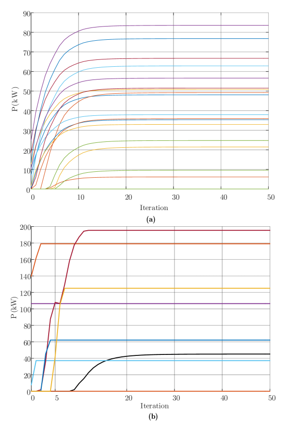
Figure 6: Generation output and load demand powers in case study I; (a) demands ($kW$), (b) DGs ($kW$)

TABLE I: The coefficients of DGs’ cost functions and consumers’ utility functions in case study I

	Cost function			Utility function
$i$	$\alpha_{i}$	$\beta_{i}$	$P_{i,max}^{Gen}$	$\omega_{i}$	$b_{i}$	$P_{i,max}^{Load}$
1	0.0031	8.71	113.23	17.17	0.0935	91.79
2	0.0074	3.53	179.1	12.28	0.0417	147.29
3	0.0066	7.58	90.03	18.42	0.1007	91.41
4	0.0063	2.24	106.41	7.06	0.0561	62.96
5	0.0069	8.53	193.80	10.85	0.0540	100.53
6	0.0014	2.25	37.19	18.91	0.1414	66.88
7	0.0041	6.29	195.4	18.76	0.0793	118.35
8	0.0051	4.30	62.17	15.70	0.1064	73.81
9	0.0032	8.26	143.41	14.28	0.0850	84.00
10	0.0025	5.3	125	10.15	0.0460	110.32
11	–	–	–	19.04	0.0650	146.46
12	–	–	–	06.87	0.0549	62.61
13	–	–	–	15.96	0.0619	128.91
14	–	–	–	14.70	0.0633	116.08
15	–	–	–	17.50	0.0607	144.04
16	–	–	–	10.97	0.2272	24.15
17	–	–	–	16.25	0.1224	66.39
18	–	–	–	17.53	0.0826	106.14
19	–	–	–	09.84	0.0869	56.60

TABLE II: Comparison of the output of DGs achieved by distributed and centralized methods in case study I

Output Power $(kW)$	Distributed Method	Centralized Method
$P_{1}$	0	0
$P_{2}$	179.1	179.099
$P_{3}$	45.16	45.1614
$P_{4}$	106.4	106.409
$P_{5}$	0	0
$P_{6}$	37.19	37.189
$P_{7}$	195.4	195.399
$P_{8}$	62.17	62.1699
$P_{9}$	0	0
$P_{10}$	125	124.999
Total	750.4	750.428

Figure 6 shows the evolution of DG power output and load demand, respectively. Figure 6(a) contains 19 consumer demand curves and Figure 6(b) includes 10 DG output-power curves. As can be seen in 6, the economic dispatch solution converges at the 36-th iteration. The corresponding execution time is about 1.69 seconds. The accuracy of the proposed distributed solution algorithm is validated by the benchmark results found by a centralized method. As shown in Tables II and III, the solution mismatch between the distributed and centralized methods is less than 0.00201% of the average. As the distributed algorithm proceeds, the incremental cost converges to $8.175\,\nicefrac{\mathrm{\$}}{\mathrm{kwh}}$, as shown in Figure 7. The evolution of power mismatch, the evolution of total generation and the evolution of total load demand are shown in Figure 8. Power mismatch ($\Delta P$) serves as coordination information and gradually converges to a consensus (i.e., $0\;kW$). The power tolerance is set to be 0.001 kW in our case studies. As the incremental cost and power mismatch settle down, the optimal value of social welfare is found to be $5,211.5\,\nicefrac{\mathrm{\$}}{\mathrm{hr}}$. It is important to note that the proposed distributed algorithm is able to converge to the near-optima much faster than other distributed methods [22, 20, 23]. For example, one of the published works [23] showed that the same economic dispatch problem was solved after 500 iterations, while our distributed control algorithm is able to find the same results at the 36-th iteration.

TABLE III: Comparison of the demand of loads achieved by distributed and centralized methods

Demand of Loads $(kW)$	Distributed Method	Centralized Method
$L_{1}$	48.1	48.095
$L_{2}$	49.21	49.207
$L_{3}$	50.86	50.863
$L_{4}$	0	0
$L_{5}$	24.76	24.758
$L_{6}$	37.96	37.955
$P_{7}$	66.73	66.733
$L_{8}$	35.36	35.356
$L_{9}$	35.91	35.905
$L_{10}$	21.46	21.455
$L_{11}$	83.57	83.568
$L_{12}$	0	0
$L_{13}$	62.87	62.874
$L_{14}$	51.53	51.531
$L_{15}$	76.8	76.80
$L_{16}$	6.148	6.148
$L_{17}$	32.98	32.981
$L_{18}$	56.62	56.621
$L_{19}$	9.573	9.573
Total	750.4	750.428

IV-B Case Study II (Evaluation of Scalability and Fast Convergence)

In order to demonstrate the scalability, we then apply the proposed solution algorithm to a large-scale system, including 1,000 consumers and 400 DGs. The initial conditions of the1,400 agents are randomly selected.

As shown in Figure 9, the incremental costs reach consensus within approximately 40 iterations, which is considered a fast convergence rate for a 1,400-agent system. The corresponding execution time is 192.579 seconds. Some simulation for different numbers of agents, 29 (10 DGs and 19 Consumers), 350 (150 DGs and 200 Consumers), 700 (300 DGs and 400 Consumers), 1050 (350 DGs and 700 Consumers), 1400 (400 DGs and 1000 Consumers), are performed to study the trend in number of iteration for convergence. The Figure 10 shows that as the number of agents increase from 29 (case study I) to 1,400 (case study II), the number of iteration is almost constant, demonstrating that the proposed distributed algorithm is particularly suitable for solving large-scale economic dispatch problems. The minimum error criteria for power mismatch tolerance is set to be $\Delta P=0.001\;kW$ in our case studies used in Figure 10.

As previously emphasized, the power mismatch is the only shared information between agents. It reduces the computational cost because the proposed algorithm only needs a simple updating process on the power mismatch. Besides, consumers do not need to establish any communication channel among themselves to coordinate any information state or with more than one DG. The above-mentioned features contribute to a significantly reduction on the computing complexity.

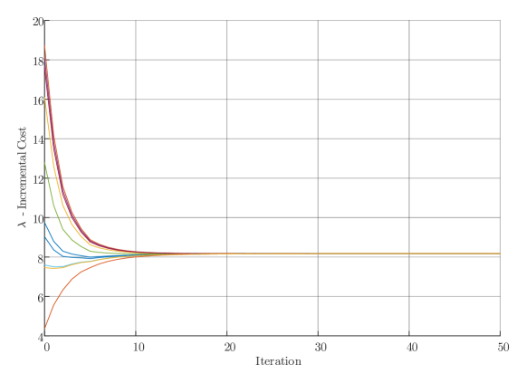
Figure 7: Incremental cost of DGs in case study I

IV-C Case Study III (Evaluation of Practical Performance)

The proposed distributed algorithm is particularly designed for easy implementation and configuration of local agents by using a simple proportional-integral (PI) or integral (I) controller. Equations (LABEL:eq:completedeltaP)-(43) can be easily modeled as a PI or I controller to update the estimated power mismatch iteratively and exchange information (i.e., $\Delta P$) with other agents. Figure 11(a) shows a simple PI controller for a DG. A PI controller is used for each consumer to adjust its own demand based on $\Delta\lambda$ between the current and previous iteration. Figure 11(b) shows a simple controller for a consumer. As $\Delta\lambda$ becomes zero, the consumer’s surplus is maximized.

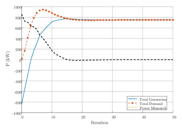
Figure 8: Generation, demand and power mismatch in case

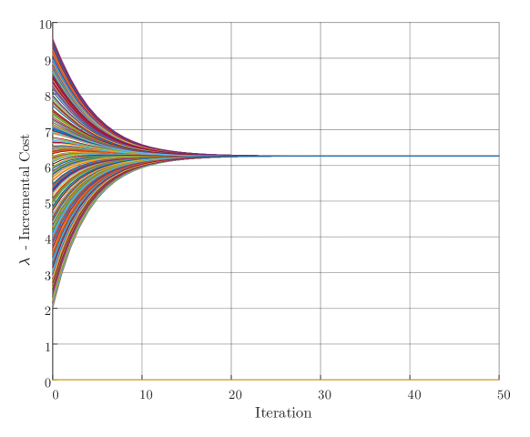
Figure 9: Incremental cost ($\nicefrac{\mathrm{\$}}{\mathrm{kWh}}$) of DGs in case study II

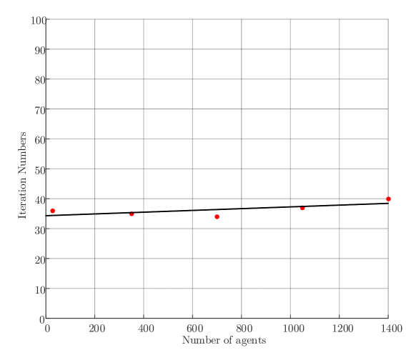
Figure 10: The trend in number of iteration for algorithm conv

In case study III, the communication platform is implemented in VOLTTRON™ which is an innovative distributed control and sensing software platform developed by the Pacific Northwest National Laboratory [42]. The open-source VOLTTRON™ platform makes it possible to deploy distributed control agents at a very low cost. The platform provides various services such as resource management, agent code verification and directory services allowing to manage different assets within the power system. In the large scale, VOLTTRON™ can manage assets within smart grids, facilitate demand response, support energy trading and record grid data.

The VOLTTRON™ platform is implemented on an ordinary Linux desktop with an FX-4100 CPU @ 3.6 GHz, 8-GB RAM memory. The control platform is substantiated into a cluster of low-cost credit-card-size single board PCs (Cubieboard A20). The Cubieboard A20 processor is based on a dual-core ARM Cortec-A7 CPU architecture. We use the Python programming language to implement the proposed consensus-based distributed control algorithms for each agent. In this proof-of-concept implementation, every Cubieboard is emulated as a distributed controller for local agents (DGs and consumers), while the PC with the VOLTTRON™ platform is regarded as an information exchange bus. The decision making process is conducted in a fully distributed fashion. Figure 12 shows the overall system set up. For the demonstration purpose, the proposed distributed algorithm is applied to a relatively small-scale distribution system including 6 DGs and 10 consumers. As shown in figure 12, DGs are labeled as G1, G2, …, G6 while consumers are labeled as L1, L2, …, L10. The coefficients of DGs’ cost functions and consumers’ utility functions are randomly selected.

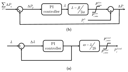
Figure 11: Local PI-controller for DGs and consumers; (a) PI-controller for DGs, (b) PI-controller for consumers

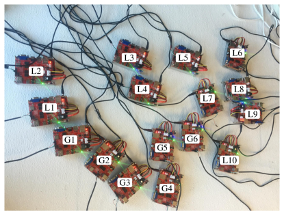
Figure 12: The Proof-of-Concept 16-node Testbed using a Cluster of Single-board PCs (“L” inidicates loads/consumers; “G” inididates DGs)

Figure 13 shows the detailed experimental test results. The output-power of DG3 and DG5 and the demand of L4 are zero. The experimental test results are validated using the benchmark results achieved by a centralized approach. As figure 13 shows, the total generation is about $421\,\mathrm{kW}$ that satisfies the total load demand. The incremental cost converges to $7.371\,\nicefrac{\mathrm{\$}}{\mathrm{kwh}}$ at the 42-th iteration, which is considered as a fast convergence rate.

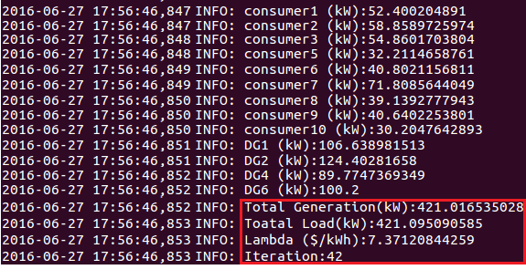
Figure 13: The experimental test results

V Conclusions

In this paper, we proposed a novel consensus-based distributed algorithm to solve an optimal dispatch problem of distributed generators. First, we formulated the social welfare problem considering the cost functions of DGs and the utility functions of consumers. Second, we developed the distributed algorithm to find the global optima by allowing the iterative coordination of agents (consumers and DGs) with each other. Agents only share their estimated power mismatch, which does not contain any private information, ultimately contributing to a fair electricity market. Third, we performed software simulation and experimental test to demonstrate the accuracy, privacy, effectiveness, fast-convergence, scalability, and easy-implementation of the proposed distributed algorithm under various conditions.

References

- [1] X. Fang, S. Misra, G. Xue, and D. Yang, “Smart grid - The new and improved power grid: A survey,” IEEE Communications Surveys and Tutorials, vol. 14, no. 4, pp. 944–980, jan 2012. [Online]. Available: http://ieeexplore.ieee.org/lpdocs/epic03/wrapper.htm?arnumber=6099519
- [2] C. W. Potter, A. Archambault, and K. Westrick, “Building a smarter smart grid through better renewable energy information,” 2009 IEEE/PES Power Systems Conference and Exposition, PSCE 2009, pp. 1–5, 2009.
- [3] Analytic Research Foundations for the Next-Generation Electric Grid. Washington, D.C.: National Academies Press, 2016. [Online]. Available: http://www.nap.edu/catalog/21919
- [4] A. Asadinejad, K. Tomsovic, and C. Chen, “Sensitivity of Incentive Based Demand Response Program To Residential Customer Elasticity,” in North American Power Symposium(NAPS). Denver, CO: IEEE, sep 2016.
- [5] R. Mudumbai, S. Dasgupta, and B. B. Cho, “Distributed control for optimal economic dispatch of a network of heterogeneous power generators,” IEEE Transactions on Power Systems, vol. 27, no. 4, pp. 1750–1760, nov 2012. [Online]. Available: http://ieeexplore.ieee.org/lpdocs/epic03/wrapper.htm?arnumber=6178300
- [6] R. Saber and R. Murray, “Consensus protocols for networks of dynamic agents,” in Proceedings of the 2003 American Control Conference, 2003., vol. 2. IEEE, 2003, pp. 951–956. [Online]. Available: http://ieeexplore.ieee.org/lpdocs/epic03/wrapper.htm?arnumber=1239709
- [7] W. Ren and R. W.Beard, Distributed consensus in multi-vechicle cooperative control, ser. Communications and Control Engineering. London: Springer London, 2008, vol. 36. [Online]. Available: http://www.ncbi.nlm.nih.gov/pubmed/24815723
- [8] R. Olfati-Saber, J. A. Fax, and R. M. Murray, “Consensus and cooperation in networked multi-agent systems,” Proceedings of the IEEE, vol. 95, no. 1, pp. 215–233, jan 2007. [Online]. Available: http://ieeexplore.ieee.org/lpdocs/epic03/wrapper.htm?arnumber=4118472
- [9] G. Binetti, A. Davoudi, F. L. Lewis, D. Naso, and B. Turchiano, “Distributed consensus-based economic dispatch with transmission losses,” IEEE Transactions on Power Systems, vol. 29, no. 4, pp. 1711–1720, 2014. [Online]. Available: http://ieeexplore.ieee.org/lpdocs/epic03/wrapper.htm?arnumber=6717171
- [10] S. Xu, H. Pourbabak, and W. Su, “Distributed cooperative control for economic operation of multiple plug-in electric vehicle parking decks,” International Transactions on Electrical Energy Systems, p. e2348, 2017. [Online]. Available: http://doi.wiley.com/10.1002/etep.2348
- [11] Y. Xu, J. Hu, W. Gu, W. Su, and W. Liu, “Real-Time Distributed Control of Battery Energy Storage Systems for Security Constrained DC-OPF,” IEEE Transactions on Smart Grid, pp. 1–1, 2016. [Online]. Available: http://ieeexplore.ieee.org/document/7523948/
- [12] Z. Zhang and M. Y. Chow, “Convergence analysis of the incremental cost consensus algorithm under different communication network topologies in a smart grid,” IEEE Transactions on Power Systems, vol. 27, no. 4, pp. 1761–1768, nov 2012. [Online]. Available: http://ieeexplore.ieee.org/lpdocs/epic03/wrapper.htm?arnumber=6183499
- [13] H. Pourbabak, T. Chen, B. Zhang, and W. Su, “Control and energy management system in microgrids,” in Clean Energy Microgrids. Institution of Engineering and Technology, 2017, ch. 3, pp. 109–133. [Online]. Available: http://digital-library.theiet.org/content/books/10.1049/pbpo090e_ch3
- [14] W. Zeng and M. Y. Chow, “Resilient distributed control in the presence of misbehaving agents in networked control systems,” IEEE Transactions on Cybernetics, vol. 44, no. 11, pp. 2038–2049, nov 2014. [Online]. Available: http://www.ncbi.nlm.nih.gov/pubmed/25330469
- [15] D. Kirschen and G. Strbac, Fundamentals of Power System Economics. Chichester, UK: John Wiley & Sons, Ltd, mar 2004, vol. 4, no. 4. [Online]. Available: http://doi.wiley.com/10.1002/0470020598
- [16] P. Samadi, H. Mohsenian-Rad, R. Schober, and V. W. S. Wong, “Advanced demand side management for the future smart grid using mechanism design,” IEEE Transactions on Smart Grid, vol. 3, no. 3, pp. 1170–1180, sep 2012. [Online]. Available: http://ieeexplore.ieee.org/lpdocs/epic03/wrapper.htm?arnumber=6266724
- [17] Y. Xu, “Optimal Distributed Charging Rate Control of Plug-In Electric Vehicles for Demand Management,” IEEE Transactions on Power Systems, vol. 30, no. 3, pp. 1536–1545, may 2015. [Online]. Available: http://ieeexplore.ieee.org/document/6889041/http://ieeexplore.ieee.org/lpdocs/epic03/wrapper.htm?arnumber=6889041
- [18] W. Ren and Y. Cao, Distributed Coordination of Multi-agent Networks, ser. Communications and Control Engineering, Intergovernmental Panel on Climate Change, Ed. London: Springer London, nov 2011, vol. 58, no. 12. [Online]. Available: http://link.springer.com/10.1007/978-0-85729-169-1
- [19] A. Kazemi and H. Pourbabak, “Islanding detection method based on a new approach to voltage phase angle of constant power inverters,” IET Generation, Transmission & Distribution, vol. 10, no. 5, pp. 1190–1198, apr 2016. [Online]. Available: http://digital-library.theiet.org/content/journals/10.1049/iet-gtd.2015.0776
- [20] F. Guo, C. Wen, J. Mao, and Y. D. Song, “Distributed Economic Dispatch for Smart Grids with Random Wind Power,” IEEE Transactions on Smart Grid, vol. 7, no. 3, pp. 1572–1583, may 2016. [Online]. Available: http://ieeexplore.ieee.org/lpdocs/epic03/wrapper.htm?arnumber=7120161
- [21] P. Yi, Y. Hong, and F. Liu, “Distributed gradient algorithm for constrained optimization with application to load sharing in power systems,” Systems & Control Letters, vol. 83, pp. 45–52, sep 2015. [Online]. Available: http://www.sciencedirect.com/science/article/pii/S0167691115001346
- [22] G. Hug, S. Kar, and C. Wu, “Consensus + Innovations Approach for Distributed Multiagent Coordination in a Microgrid,” IEEE Transactions on Smart Grid, vol. 6, no. 4, pp. 1893–1903, jul 2015. [Online]. Available: http://ieeexplore.ieee.org/lpdocs/epic03/wrapper.htm?arnumber=7098427
- [23] N. Rahbari-Asr, U. Ojha, Z. Zhang, and M. Y. Chow, “Incremental welfare consensus algorithm for cooperative distributed generation/demand response in smart grid,” IEEE Transactions on Smart Grid, vol. 5, no. 6, pp. 2836–2845, nov 2014. [Online]. Available: http://ieeexplore.ieee.org/lpdocs/epic03/wrapper.htm?arnumber=6884808
- [24] N. Rahbari-Asr and M. Y. Chow, “Cooperative distributed demand management for community charging of PHEV/PEVs based on KKT conditions and consensus networks,” IEEE Transactions on Industrial Informatics, vol. 10, no. 3, pp. 1907–1916, 2014. [Online]. Available: http://ieeexplore.ieee.org/lpdocs/epic03/wrapper.htm?arnumber=6730946
- [25] E. Dall’Anese, H. Zhu, and G. B. Giannakis, “Distributed optimal power flow for smart microgrids,” IEEE Transactions on Smart Grid, vol. 4, no. 3, pp. 1464–1475, 2013.
- [26] R. Deng, Z. Yang, F. Hou, M. Chow, and J. Chen, “Distributed Real Time Demand Response in Multiseller Multibuyer Smart Distribution Grid,” IEEE Transactions on Power Systems, vol. 30, no. 5, pp. 2364–2374, sep 2015. [Online]. Available: http://ieeexplore.ieee.org/document/6922169/
- [27] W. T. Elsayed and E. F. El-Saadany, “A Fully Decentralized Approach for Solving the Economic Dispatch Problem,” IEEE Transactions on Power Systems, vol. 30, no. 4, pp. 2179–2189, jul 2014. [Online]. Available: http://ieeexplore.ieee.org/lpdocs/epic03/wrapper.htm?arnumber=6917059
- [28] W. Zhang, W. Liu, X. Wang, L. Liu, and F. Ferrese, “Online optimal generation control based on constrained distributed gradient algorithm,” IEEE Transactions on Power Systems, vol. 30, no. 1, pp. 35–45, jan 2015. [Online]. Available: http://ieeexplore.ieee.org/lpdocs/epic03/wrapper.htm?arnumber=6810888
- [29] S. Yang, S. Tan, and J.-X. Xu, “Consensus Based Approach for Economic Dispatch Problem in a Smart Grid,” IEEE Transactions on Power Systems, vol. 28, no. 4, pp. 4416–4426, 2013. [Online]. Available: http://ieeexplore.ieee.org/lpdocs/epic03/wrapper.htm?arnumber=6560423
- [30] N. Cai, N. T. T. Nga, and J. Mitra, “Economic dispatch in microgrids using multi-agent system,” in 2012 North American Power Symposium, NAPS 2012. IEEE, sep 2012, pp. 1–5. [Online]. Available: http://ieeexplore.ieee.org/lpdocs/epic03/wrapper.htm?arnumber=6336435
- [31] G. Binetti, A. Davoudi, D. Naso, B. Turchiano, and F. L. Lewis, “A distributed auction-based algorithm for the nonconvex economic dispatch problem,” IEEE Transactions on Industrial Informatics, vol. 10, no. 2, pp. 1124–1132, 2014.
- [32] T.-H. Chang, A. Nedic, and A. Scaglione, “Distributed Constrained Optimization by Consensus-Based Primal-Dual Perturbation Method,” IEEE Transactions on Automatic Control, vol. 59, no. 6, pp. 1524–1538, jun 2014. [Online]. Available: http://ieeexplore.ieee.org/document/6748910/
- [33] H. Pourbabak, Tao Chen, and W. Su, “Consensus-based distributed control for economic operation of distribution grid with multiple consumers and prosumers,” in 2016 IEEE Power and Energy Society General Meeting (PESGM), IEEE. Boston, MA, July 17-21, 2016: IEEE, jul 2016, pp. 1–5. [Online]. Available: http://ieeexplore.ieee.org/document/7741083/
- [34] M. Fahrioglu and F. Alvarado, “Using utility information to calibrate customer demand management behavior models,” IEEE Transactions on Power Systems, vol. 16, no. 2, pp. 317–322, may 2001. [Online]. Available: http://ieeexplore.ieee.org/lpdocs/epic03/wrapper.htm?arnumber=918305http://ieeexplore.ieee.org/document/918305/
- [35] P. Samadi, A.-H. Mohsenian-Rad, R. Schober, V. W. S. Wong, and J. Jatskevich, “Optimal Real-Time Pricing Algorithm Based on Utility Maximization for Smart Grid,” 2010 First IEEE International Conference on Smart Grid Communications, pp. 415–420, 2010. [Online]. Available: http://ieeexplore.ieee.org/lpdocs/epic03/wrapper.htm?arnumber=5622077
- [36] S. Mohajeryami, I. N. Moghaddam, M. Doostan, B. Vatani, and P. Schwarz, “A novel economic model for price-based demand response,” Electric Power Systems Research, vol. 135, pp. 1–9, jun 2016. [Online]. Available: http://linkinghub.elsevier.com/retrieve/pii/S0378779616300736
- [37] T. J. Nechyba, Microeconomics: An Intuitive Approach With Calculus. Cengage Learning, 2010. [Online]. Available: http://books.google.com/books?id=T4WuH3PRtYkC&pgis=1
- [38] F. L. Lewis, H. Zhang, K. Hengster-Movric, and A. Das, Cooperative Control of Multi-Agent Systems, ser. Communications and Control Engineering. London: Springer London, 2014, vol. 1542. [Online]. Available: http://link.springer.com/10.1007/978-1-4471-5574-4
- [39] S. P. Boyd and L. Vandenberghe, Convex optimization. Cambridge UK ;New York: Cambridge University Press, 2004.
- [40] A. Ruszczynski, Nonlinear Optimization. Princeton University Press, 2006.
- [41] J. Lofberg, “YALMIP : a toolbox for modeling and optimization in MATLAB,” in 2004 IEEE International Conference on Computer Aided Control Systems Design. IEEE, 2004, pp. 284–289. [Online]. Available: http://ieeexplore.ieee.org/lpdocs/epic03/wrapper.htm?arnumber=1393890
- [42] Jingwei Luo, H. Pourbabak, and W. Su, “The application of distributed control algorithms using VOLTTRON-based software platform,” in 2017 8th International Renewable Energy Congress (IREC). Dead Sea, Jordan: IEEE, mar 2017, pp. 1–6. [Online]. Available: http://ieeexplore.ieee.org/document/7926056/