Running of the Spectrum of Cosmological Perturbations in String Gas Cosmology

Abstract

We compute the running of the spectrum of cosmological perturbations in String Gas Cosmology, making use of a smooth parametrization of the transition between the early Hagedorn phase and the later radiation phase. We find that the running has the same sign as in simple models of single scalar field inflation. Its magnitude is proportional to $(1-n_{s})$ ($n_{s}$ being the slope index of the spectrum), and it is thus parametrically larger than for inflationary cosmology, where it is proportional to $(1-n_{s})^{2}$.

I Introduction

String Gas Cosmology (SGC) BV is a scenario of early universe cosmology based on fundamental principles of superstring theory (for reviews see e.g. SGCrevs ). It is assumed that the early universe is a hot gas of fundamental superstrings on a spatial manifold of compact topology. In this case, it can be shown that the T-duality symmetry of string theory (see e.g. Pol ) implies that the temperature has the following symmetry

$$T(R)\,=\,T\left(\frac{1}{R}\right)$$ (1)

where $R$ is the radius of the spatial torus measured in units of the string length.

More generally, there is a maximal temperature for a gas of fundamental strings in thermal equilibrium, the Hagedorn temperature $T_{H}$ Hagedorn . In the presence of the duality symmetry (1) a plot of temperature as a function of $R$ will have the form given in Fig. 1, with a characteristic plateau where $T\sim T_{H}$ whose width depends on the total entropy of the system BV . This is the Hagedorn phase.

Figure 1: T versus $\log{R}$ for Heteroic superstrings. Different curves are obtained for different values of the entropy - the larger the entropy the larger the plateau.

It is natural BV to expect the self-dual point $R=1$ to be a metastable fixed point. If we follow the evolution starting from a hot gas of strings, we expect the radius $R$ to remain approximately constant for a long period of time until in three spatial dimensions the winding modes annihilate into string loops, allowing the scale factor $a(t)$ of those dimensions of space to expand, as illustrated in Fig. 2.

Figure 2: Sketch of the evolution of the scale factor $a(t)$ (vertical axis) as a function of time $t$ (horizontal axis). The time $t_{R}$ denotes the end of the Hagedorn phase.

As first discussed in NBV , string gas cosmology leads to a theory for the origin of structure in the universe which is different from the inflationary universe scenario. The relevant space-time diagram is sketched in Fig. 3. Here, the vertical axis is time, and the horizontal axis represents distance in physical coordinates. The heavy solid curve represents the Hubble radius $H^{-1}(t)$ which is infinite in the Hagedorn and expands as in Standard Big Bang cosmology after the phase transition is completed. As is evident, all length scales $k$ ($k$ denoting the comoving wavenumber) start their evolution inside the Hubble radius. They exit the Hubble radius at a time $t_{H}(k)$ which is close to the time $t_{R}$ but increases slightly as $k$ increases. Since the Hagedorn phase is filled with a hot gas of fundamental strings, the fluctuations in this phase will be thermal fluctuations of a string gas.

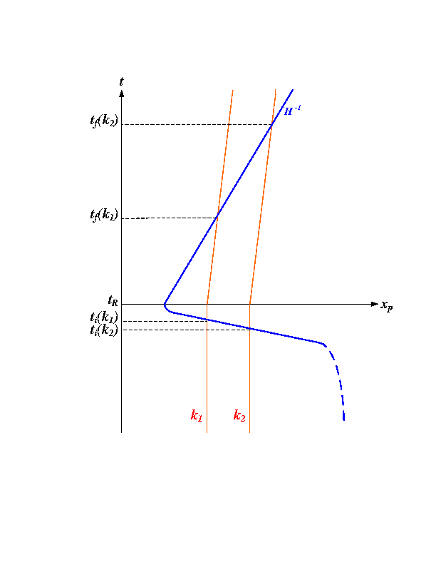
Figure 3: Space-time sketch of string gas cosmology. The vertical axis is time, with $t_{R}$ denoting the end of the Hagedorn phase. The period $t<t_{R}$ corresponds to the quasi-static Hagedorn phase, the period $t>t_{R}$ to the radiation-dominated phase of expansion of Standard Big Bang cosmology. The horizontal axis is physical length. The heavy solid line represents the Hubble radius, the light solid lines which are vertical for $t<t_{R}$ correspond to the wavelengths corresponding to various comoving wavenumbers $k$. The wavelength equals the Hubble radius (the modes “exit” the Hubble radius) at a time $t_{H}(k)$ and then re-enter late in the phase of Standard cosmology.

From Fig. 3 it is clear that all scales originate inside the Hubble radius. Hence, it is possible to have a causal structure formation scenario, as in the case of inflationary cosmology. In contrast to the case of inflation, however, the fluctuations are thermal and not vacuum since the state of matter in the Hagedorn phase is a hot gas of strings. As was shown in NBV (see also Nayeri ; BNPV1 ), thermal fluctuations of strings in the Hagedorn phase lead to an approximately scale-invariant spectrum of cosmological perturbations. The amplitude of the spectrum on a scale $k$ is set by NBV $(1-T/T_{H})^{-1}$, where $T$ is the temperature when the mode $k$ exits the Hubble radius. Since this temperature decreases as $k$ increases, a slight red tilt of the spectrum results.

SGC also generates gravitational waves. Their amplitude is set by the factor $(1-T/T_{H})$ BNPV2 , and hence the spectrum - while approximately scale-invariant - has a slight blue tilt, in contrast to inflationary scenarios where a red tilt is predicted . Thus, the tilt of the gravitational wave spectrum is a key characteristic of SGC.

There are two free parameters in SGC: the ratio of the string length to the Planck length, and the the value of $(1-\frac{T}{T_{H}})$ during the Hagedorn phase. These parameters can be fit to the observed amplitude and slope of the spectrum of scalar metric fluctuations. Then, the tensor to scalar ratio $r$ and the slope of the tensor spectrum $n_{t}$ are determined. One obtains

$$n_{t}\,\simeq\,(1-n_{s})\,,$$ (2)

where $n_{s}$ is the slope of the scalar spectrum. However, the value of $r$ is predicted to be well below the current observational limits. Hence, we are currently not able to test the consistency relation (2), and we will not be able to in the near future. Hence, it is interesting to search for other ways to observationally distinguish between the predictions of SGC and those of simple single field slow-roll inflation models.

In this paper we study the running of the spectrum of cosmological perturbations. The running has recently been shown to be a diagnostic to differentiate between inflationary models and matter bounce cosmologies EWE (see e.g. BP for a recent review of bouncing models). Whereas the running has a negative sign in the case of inflation, it has a typical positive sign in the case of a matter bounce model. In the present work we compute the running of the spectrum assuming a simple smooth transition between the Hagedorn phase and the expanding radiation phase of Standard Big Bang cosmology. We find that the running has the same sign as in the case of inflation, but that it is parametrically larger. In the case of inflation one has (see e.g. EWE )

$$\alpha_{s}\,\sim\,-(n_{s}-1)^{2}\,$$ (3)

whereas SGC predicts

$$\alpha_{s}\,\sim\,-(1-n_{s})\,.$$ (4)

This consistency relation is much easier to confront with observational results.

II Setup

The slope and running of the spectrum of cosmological perturbations are defined by

$$n_{s}-1\, \equiv \,\frac{d\text{lnP}_{\Phi}(k)}{d\text{ln}k}|_{k=aH}\,=\,\frac{k}{P_{\Phi}}\frac{dP_{\Phi}}{dk}$$ (5)

$$\alpha_{s}\, \equiv \frac{d^{2}\text{ln}P_{\Phi}(k)}{d\text{ln}k^{2}}|_{k=aH}$$

$$= \,\frac{k}{P_{\Phi}}\frac{dP_{\Phi}}{dk}-\left(\frac{k}{P_{\Phi}}\frac{dP_{\Phi}}{dk}\right)^{2}+\frac{k^{2}}{P_{\Phi}}\frac{d^{2}P_{\Phi}}{dk^{2}}\,.$$

In the above, $P_{\Phi}$ is the dimensionless power spectrum of the relativistic potential $\Phi({\bf x},t)$ which in longitudinal gauge characterizes the fluctuation of the metric in the following way (see e.g. MFB )

$$ds^{2}\,=\,-(1+2\Phi)dt^{2}+(1-2\Phi)a^{2}(t)\delta_{ij}dx^{i}dx^{j}\,,$$ (7)

where $ds$ is the proper distance, $t$ is physical time and $x^{i}$ are the comoving spatial coordinates (the index $i$ runs over the spatial indices 1,2,3 and $\delta_{ij}$ is the usual Kronecker delta symbol). The symbol $k$ stands for the comoving momentum magnitude (we are assuming spatial isotropy), and we are evaluating the derivatives at the Hubble scale (our pivot scale).

The current constraints (68% confidence levels) on the slope and the running from the Planck temperature and lensing analysis Planck are

$$n_{s}-1\, = \,-0.032\pm 0.006$$ (8)

$$\alpha_{s}\, = \,-0.003\pm 0.007\,.$$ (9)

Note that in deriving these constraints it is assumed that the contribution of gravitational waves to the spectrum of fluctuations is negligible, which is not a good approximation in SGC. Hence, the effective error bars are larger.

In a typical slow roll inflation, the power spectrum of the curvature perturbation ${\mathcal{R}}$ (which up to a numerical constant equals the potential $\Phi$ at late times) has the form:

$$\mathcal{P}_{\mathcal{R}}(k)\,=\,\frac{H^{2}}{\epsilon}$$ (10)

where the right-hand side is evaluated when the scale $k$ exits the Hubble radius during inflation, and $\epsilon\equiv-dlnH/dlna$ is the slow roll parameter. Using the e-folding number $N$ as the time parameter, $\epsilon$ can be parametrized as (see e.g. Mukh2 )

$$\epsilon(N)\,=\,\frac{1}{(N+1)^{p}}\,,$$ (11)

where $p=1$ for chaotic inflation Linde and $p=2$ for plateau inflation Starob . The spectral index and running then take on the following form (see e.g. Limin )

$$n_{s}-1\, = \,-2\epsilon+\frac{\epsilon,_{\mathcal{N}}}{\epsilon}$$

$$=\,-\frac{2}{(\mathcal{N}+1)^{p}}-\frac{p}{\mathcal{N}+1}$$

$$\alpha_{s}\, = \,2\epsilon,_{\mathcal{N}}-\frac{\epsilon,{{}_{\mathcal{NN}}}}{\epsilon}+(\frac{\epsilon,_{N}}{\epsilon})^{2}$$ (13)

$$=\,-\frac{2p}{(\mathcal{N}+1)^{p+1}}-\frac{p}{(\mathcal{N}+1)^{2}}\,.$$

and this will then yield the quadratic relation (3) between the running $\alpha_{s}$ and $n_{s}-1$. A small deviation of the spectrum from scale-invariance will lead to a very small running of the spectrum.

As we show in the following section, the result in string gas cosmology is different.

III Analysis

In string gas cosmology the fluctuations are of thermal origin. As derived in NBV , the spectrum of cosmological perturbations on a scale $k$ is given by

$$P_{\Phi}(k)\,=\,16\pi^{2}G^{2}\frac{T(k)}{l_{s}^{3}}\frac{1}{1-T(k)/T_{H}}\,\approx\,C\frac{1}{\epsilon(k)}$$ (14)

where $C$ is a constant and we have defined

$$\epsilon(k)\,\equiv\,\left(1-\frac{T(k)}{T_{H}}\right)\,.$$ (15)

Here, $T(k)$ is the temperature of the string gas when the scale $k$ exits the Hubble radius at the end of the Hagedorn phase (see Fig. 3).

Since all scales exit the Hubble radius at temperatures close to the Hagedorn temperature, the overall shape of the spectrum is scale-invariant. Since modes with larger values of $k$ exit slightly later, when the temperature is slightly lower, the value of $\epsilon$ is slightly larger, and thus a slight red tilt of the spectrum results, as in inflationary cosmology. Here, we wish to compute the running of the spectrum.

Quantitatively, from (14) and from the definitions of the slope and running of the spectrum we obtain

$$n_{s}-1\, \simeq \,-\frac{\epsilon^{\prime}}{\epsilon}$$ (16)

$$\alpha_{s}\, \simeq \,-\frac{\epsilon^{\prime\prime}\epsilon-(\epsilon^{\prime})^{2}}{\epsilon^{2}}\,,$$ (17)

where the prime indicates a derivative with respect to ${\rm ln}k$. In the above, the value of $\epsilon(k)$ is determined by $\epsilon(T_{H}(k))$, where $T_{H}(k)$ is the temperature when the mode $k$ exits the Hubble radius.

Unfortunately the dynamics of space-time during the Hagedorn phase is not yet known. Hence, we need to resort to a parametrization of the dynamics, based on the thermodynamics of a gas of strings represented in Fig. 1, and the evolution of the scale factor assumed (see Fig. 2).

In the Hagedorn phase, the radius of our universe is constant, while in the radiation-dominated phase, the scale factor increases with time like $R(t)\sim t^{1/2}$. We first use a quadratic polynomial to connect the two phases. We take the time $t=0$ to be the end of the Hagedorn phase, and $t_{0}$ to be the end of the transition phase:

$$R(t)=\left\{\begin{aligned} &c,&t\leqslant 0\\ &c+\alpha\left(\frac{t}{t_{0}}\right)^{2},&0<t\leqslant t_{0}\\ &c+\beta\left(\frac{t}{t_{0}}+\gamma\right)^{1/2},&t>t_{0}\end{aligned}\right.$$ (18)

where $\beta=2\alpha$ to make the function continuous. In addition, we can choose $\gamma=-3/4$ to render the first derivative continuous at $t_{0}$ .

In the expressions (16) and (17) for the slope and the running of the spectrum, $\epsilon(k)$ is evaluted at the temperature when the mode $k$ exits the Hubble radius. We can thus relate the derivative with respect to $k$ with a derivative with respect to radius $R$ (the scale factor). We can then use the Hubble radius crossing condition

$$kR^{-1}\,=\,\frac{{\dot{R}}}{R}$$ (19)

and the expression for $R(t)$ to relate the derivative of $R$ with respect to $k$ by the derivative of $t_{H}(k)$ with respect to $k$, namely

$$\frac{\partial R}{\partial k}\,=\,k\frac{\partial t}{\partial k}$$ (20)

where $t=t_{H}(k)$. Combining these results we then obtain

$$n_{s}-1\, \approx \,-\frac{d\text{ln}\epsilon}{d\text{ln}k}=-\frac{k}{\epsilon}\frac{d\epsilon}{dR}_{|R_{0}}\frac{dR}{dk}\,=\,-\frac{k^{2}}{\epsilon}\beta_{1}\frac{dt}{dk}$$ (21)

$$\alpha_{s}\, \approx \,-\frac{d^{2}\text{ln}\epsilon}{d\text{ln}k^{2}}$$

$$= \,(n_{s}-1)\left(2+k\frac{d^{2}t}{dk^{2}}\right)+(n_{s}-1)^{2}\left(1-\frac{\epsilon\beta_{2}}{\beta_{1}^{2}}\right)$$

where $\beta_{1}$ and $\beta_{2}$ are first and second derivative of $\epsilon(R)$, evaluated at the pivot scale $R_{0}$, and they are simply related to the first and second time derivatives of the temperature function $T(R)$ after multiplying by $-T_{H}$. Large length scales such as those which are probed in cosmological observations exit the Hubble radius early, when $T(k)$ is close to the Hagedorn temperature. From the shape of $T(R)$ in Fig. 1 it then follows that both $\beta_{1}$ and $\beta_{2}$ are positive numbers. Making use of

$$t_{H}(k)\,=\,\frac{t_{0}^{2}}{2\alpha}k$$ (23)

we finally get

$$n_{s}-1=-\frac{k^{2}}{\epsilon}\frac{t_{0}^{2}}{2\alpha}\beta_{1}$$ (24)

$$\alpha_{s}=-\frac{k^{2}}{\epsilon}\frac{t_{0}^{2}}{2\alpha}2\beta_{1}+\left(\frac{k^{2}}{\epsilon}\frac{t_{0}^{2}}{2\alpha}\beta_{1}\right)^{2}\left(1-\frac{\epsilon\beta_{2}}{\beta_{1}^{2}}\right)\,.$$

Since $\beta_{1}$ and $\beta_{2}$ are both positive, we get a negative running. and, Since $n_{s}-1\approx-0.03$ from the most recent CMB data, the $(n_{s}-1)^{2}$ terms are negligible. Hence we predict a linear relation between $n_{s}-1$ and $\alpha_{s}$ as in (4).

We also considered a more general parametrization of $R(t)$ in which R is proportional to $(t/t_{0})^{n}$, and we get a similar linear relation

$$\alpha_{s}\,=\,(n_{s}-1)\left[2-\frac{n-2}{n-1}+(n_{s}-1)\left(1-\frac{\epsilon\beta_{2}}{\beta_{1}^{2}}\right)\right]$$ (25)

between the running and the tilt of the spectrum. Different models just influence the $\mathcal{O}(1)$ coefficient in the linear relation between running and spectral index. Note that if $n$ is negative, a blue spectrum of cosmological perturbations results.

IV Conclusions and Discussion

In conclusion, we have calculated the running of the power spectrum in string gas cosmology (SGC) and obtain a negative running. In addition, our parametrizations of $R(t)$ and $T(R)$ yield a linear relationship between the spectral index and running. This string gas cosmology consistency relation is already in the realm of what can be tested with current data. In fact, it may appear that our predictions are already in tension with the latest Planck results. However, in string gas cosmology the contribution of gravitational waves is not negligible, and hence the limits of Planck are not directly applicable. It would be interesting to do an analysis of the current data allowing amplitude, slope, running and gravitational wave contributions to all vary as predicted in SGC.

While we have presented our results for specific parametrizations of $R(t)$ and $T(t)$, our main result - namely the linear dependence of the running of the spectrum on the deviation of the spectrum from scale-invariance - is quite general. We have explored an extended space of parametrizations. Note that since we care most about the large scale perturbations, we focus on $t\sim 0$. In particular, it can be shown that for an arbitrary interpolation function between the two phases we still obtain a linear relation between the running and $n_{s}-1$, having different interpolation functions influencing only the $\mathcal{O}(1)$ coefficient.

Given we are predicting a linear relation between running and slope of the spectrum of cosmological perturbations, let us step back and ask why one obtains a quadratic relation (3) in simple inflationary models: Take a back at the equation (II), we find that $\frac{d^{2}P_{\Phi}}{dk^{2}}k^{2}/P_{\Phi}$ is positive in inflation and cancels against the first term, leaving the second term which is approximately proportional to $|n_{s}-1|^{2}$. But in string gas model, both the first term and the third term are negative, and hence there is no cancellation. Considering that the second term is proportional to $|n_{s}-1|^{2}$ it will be negligible compared to the first term. However, to make a quick transition, $\beta_{2}$ should be a large amount, thus we cannot neglect the third term. If we suppose that $\beta_{2}$ is small, corresponding to a smooth and slow transition, this will give us the prediction $|\alpha_{s}|\sim|n_{s}-1|$.

References

- (1) R. H. Brandenberger and C. Vafa, “Superstrings In The Early Universe,” Nucl. Phys. B 316, 391 (1989).
-
(2)
R. H. Brandenberger, “String Gas Cosmology: Progress
and Problems,” Class. Quant. Grav. 28, 204005 (2011)
doi:10.1088/0264-9381/28/20/204005 [arXiv:1105.3247 [hep-th]];
R. H. Brandenberger, “String Gas Cosmology,” String Cosmology, J.Erdmenger (Editor). Wiley, 2009. p.193-230 [arXiv:0808.0746 [hep-th]];
T. Battefeld and S. Watson, “String gas cosmology,” Rev. Mod. Phys. 78, 435 (2006) [arXiv:hep-th/0510022]. -
(3)
J. Polchinski,
“String theory. Vol. 1: An introduction to the bosonic string,”;
J. Polchinski, “String theory. Vol. 2: Superstring theory and beyond,” - (4) R. Hagedorn, “Statistical Thermodynamics Of Strong Interactions At High-Energies,” Nuovo Cim. Suppl. 3, 147 (1965).
- (5) A. Nayeri, R. H. Brandenberger and C. Vafa, “Producing a scale-invariant spectrum of perturbations in a Hagedorn phase of string cosmology,” Phys. Rev. Lett. 97, 021302 (2006) [arXiv:hep-th/0511140].
- (6) A. Nayeri, “Inflation Free, Stringy Generation of Scale-Invariant Cosmological Fluctuations in D = 3 + 1 Dimensions,” hep-th/0607073.
- (7) R. H. Brandenberger, A. Nayeri, S. P. Patil and C. Vafa, “String gas cosmology and structure formation,” Int. J. Mod. Phys. A 22, 3621 (2007) [hep-th/0608121].
-
(8)
R. H. Brandenberger, A. Nayeri, S. P. Patil and C. Vafa,
“Tensor Modes from a Primordial Hagedorn Phase of String Cosmology,”
Phys. Rev. Lett. 98, 231302 (2007)
doi:10.1103/PhysRevLett.98.231302
[hep-th/0604126];
R. H. Brandenberger, A. Nayeri and S. P. Patil, “Closed String Thermodynamics and a Blue Tensor Spectrum,” Phys. Rev. D 90, no. 6, 067301 (2014) doi:10.1103/PhysRevD.90.067301 [arXiv:1403.4927 [astro-ph.CO]]. - (9) T. Kobayashi, M. Yamaguchi and J. Yokoyama, “G-inflation: Inflation driven by the Galileon field,” Phys. Rev. Lett. 105, 231302 (2010) doi:10.1103/PhysRevLett.105.231302 [arXiv:1008.0603 [hep-th]].
- (10) M. He, J. Liu, S. Lu, S. Zhou, Y. F. Cai, Y. Wang and R. Brandenberger, “Differentiating G-inflation from String Gas Cosmology using the Effective Field Theory Approach,” JCAP 1612, 040 (2016) doi:10.1088/1475-7516/2016/12/040 [arXiv:1608.05079 [astro-ph.CO]].
- (11) J. L. Lehners and E. Wilson-Ewing, “Running of the scalar spectral index in bouncing cosmologies,” JCAP 1510, no. 10, 038 (2015) doi:10.1088/1475-7516/2015/10/038 [arXiv:1507.08112 [astro-ph.CO]].
- (12) R. Brandenberger and P. Peter, “Bouncing Cosmologies: Progress and Problems,” Found. Phys. 47, no. 6, 797 (2017) doi:10.1007/s10701-016-0057-0 [arXiv:1603.05834 [hep-th]].
- (13) V. F. Mukhanov, H. A. Feldman and R. H. Brandenberger, “Theory of cosmological perturbations. Part 1. Classical perturbations. Part 2. Quantum theory of perturbations. Part 3. Extensions,” Phys. Rept. 215, 203 (1992). doi:10.1016/0370-1573(92)90044-Z
- (14) P. A. R. Ade et al. [Planck Collaboration], “Planck 2015 results. XX. Constraints on inflation,” Astron. Astrophys. 594, A20 (2016) doi:10.1051/0004-6361/201525898 [arXiv:1502.02114 [astro-ph.CO]].
- (15) V. Mukhanov, “Quantum Cosmological Perturbations: Predictions and Observations,” Eur. Phys. J. C 73, 2486 (2013) doi:10.1140/epjc/s10052-013-2486-7 [arXiv:1303.3925 [astro-ph.CO]].
- (16) A. D. Linde, “Chaotic Inflation,” Phys. Lett. 129B, 177 (1983). doi:10.1016/0370-2693(83)90837-7
- (17) A. A. Starobinsky, “A New Type of Isotropic Cosmological Models Without Singularity,” Phys. Lett. 91B, 99 (1980). doi:10.1016/0370-2693(80)90670-X
- (18) L. M. Wang, V. F. Mukhanov and P. J. Steinhardt, “On the problem of predicting inflationary perturbations,” Phys. Lett. B 414, 18 (1997) doi:10.1016/S0370-2693(97)01166-0 [astro-ph/9709032].