CERN-TH-2017-162

We consider constraints on the S-matrix of any gapped, Lorentz invariant quantum field theory in 3+1 dimensions due to crossing symmetry, analyticity and unitarity. We extremize cubic couplings, quartic couplings and scattering lengths relevant for the elastic scattering amplitude of two identical scalar particles. In the cases where our results can be compared with the older S-matrix literature they are in excellent agreement. We also extremize a cubic coupling in 2+1 dimensions which we can directly compare to a universal bound for a QFT in AdS. This paper generalizes our previous 1+1 dimensional results of [1] and [2].

1 Introduction

In [1] and [2] we initiated a bootstrap analysis of massive quantum field theories. In particular, we obtained bounds on couplings of a quantum field theory compatible with a given spectrum of stable particles.

Physically, one expects such bounds to exist since increasing the interaction strength will typically increase the attraction between particles. As such, we expect to have maximum values for couplings beyond which the masses of bound states must decrease, or new bound-states should emerge from the continuum, or both.

Mathematically, this problem is also very natural once we make the non-trivial assumption that scattering amplitudes are described by functions that are analytic away from the usual physical poles and cuts. The point is that analytic functions always attain their maximum at a boundary of their domain of definition. In the context of scattering amplitudes, these boundaries are the cuts generated by multiparticle intermediate states. For physical kinematics the amplitude along the cut is constrained by the conditions that probabilities add up to one – i.e. by unitarity. For this reason we focus on the two body scattering of the lightest particle in the theory since then all the usual cuts of the amplitude correspond to physical kinematics. In $1+1$ dimensions where unitarity can be directly applied at the level of the S-matrix (simply, $|S(s)|\leq 1$ for $s$ along the cuts) we are faced with a clean problem in the theory of complex functions of a single variable. As we have an analytic function on a domain with a boundary along which it is bounded, so we are able to constrain its values inside this region and in particular the various physical couplings which we define as residues of factorization poles. Section 2 contains a derivation of the two dimensional bound which is a significant refinement of that in [2].

In this paper we move the focus to higher dimensions which contains a plethora of very interesting and difficult elements absent in the simpler $1+1$ dimensional case. An essential difference is that the most convenient way to formulate unitarity requires introducing partial waves and these are not bounded by unitarity along their entire boundary (only along the so-called “right cut”). Therefore the simple complex analysis argument of $1+1$ dimensions cannot directly apply. Furthermore, the analyticity and crossing symmetry requirements involve the amplitudes rather than the partial waves, which forces one to use both descriptions of the scattering event. Still, it is possible to overcome these technical obstacles. We shall introduce a kind of uniformization coordinates where the full space of physical kinematics is mapped to (a few) unit circles. This will allow us to Taylor expand the amplitudes in a convergent and manifestly crossing symmetric way in the full physical plane and then to numerically impose unitarity along the physical boundaries.

We start by revisiting the two dimensional results with this new approach in section 2, setup the higher dimensional problem in section 3 and present and analyze the corresponding numerical results in section 4. In section 4.4 we compare our numerical results with the completely orthogonal approach of [1] which is based on QFT in AdS and in particular does not require any analyticity assumptions. We conclude in section 5. A number of appendices are included to complement the main text presentation.

2 Two Dimensions Redux and Unit Circles

In this section we revisit the much simpler two dimensional problem. In two dimensions we can solve things analytically, and so it is a great training ground for developing intuition and testing any new numerical approaches. Nonetheless, for the braver readers eager to learn about the higher dimensional story, this section can be skipped without compromising the logic of the paper.

Most of the mathematical analysis of [2] boils down to minor variations of the following simple problem:

• Consider all real analytic functions $f(z)=\left[f(z^{\star})\right]^{\star}$ with no singularities inside the unit disk apart from a simple pole at $z=0$ and which are bounded on the unit circle as $|f(e^{i\phi})|\leq 1$. What is the maximum possible residue at $z=0$ and which function has that residue?

• The maximum residue is $1$ and the corresponding function is $f=1/z$.

Indeed $g(z)=f(z)/(1/z)$ has no singularities inside the disk and obeys $|g(z)|\leq 1$ at the boundary of the unit disk. By the so-called maximum modulus principle, it satisfies $|g(z)|\leq 1$ everywhere inside the disk. Its value at the origin – which is nothing but the residue of $f$ – is therefore at most $1$. This maximum value is attained when $g$ is constant everywhere, that is when $g(z)=1$ corresponding to $f(z)=1/z$.

Figure 1: Mapping from the cut $s$-plane to the unit disk given in equation (1). The mapping associates the points $z(2+iy)=z(2-iy)$ and maps the half plane $\text{Re}(s)>2$ to the full unit disk. The grey, dashed curves on the left map to those on the right and are included to help the reader visualize the mapping.

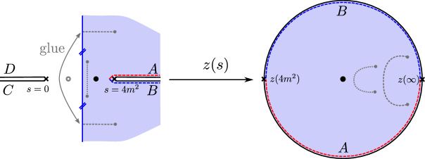
To see how this simple problem relates to the analysis in [2, 3] consider the $2\to 2$ S-matrix $S(s)$ for scattering of identical neutral particles of mass $m$ considered in [2]. Assume also that there is a single bound-state showing up in this S-matrix element and for simplicity assume its mass $m_{b}>\sqrt{2}m$. Because of crossing symmetry $S(s)=S(4m^{2}-s)$ and we can focus on the region $\mbox{Re}(s)>2m^{2}$ without any loss of generality. In this half plane we have a threshold cut starting at $s=4m^{2}$, the bound-state pole at $s=m_{b}^{2}$ and no other singularities. Consider then the change of variable

$$z=\frac{\sqrt{s(4m^{2}-s)}-m_{b}\sqrt{4m^{2}-m_{b}^{2}}}{\sqrt{s(4m^{2}-s)}+m_{b}\sqrt{4m^{2}-m_{b}^{2}}}\qquad\text{or}\qquad\Big{(}\frac{s-2m^{2}}{2m^{2}}\Big{)}^{\!\!2}\!=1+\frac{m_{b}^{2}}{m^{2}}{\Big{(}\frac{m_{b}^{2}}{4m^{2}}-1\Big{)}}\Big{(}\frac{z+1}{z-1}\Big{)}^{2}$$ (1)

which maps this half plane into the unit disk, the bound-state pole into the origin of that disk and finally the threshold cut – where unitarity is to be imposed – to the boundary of the disk, see figure 1. In terms of $z$ the S-matrix is therefore exactly constrained by the conditions of the previous point; it has a pole at $z=0$ and obeys $|S(z)|\leq 1$ at the boundary of the disk. Its maximum residue – which is where we measure the (square of the) coupling to the bound-state – is therefore $1$ and the corresponding optimal S-matrix is therefore $S(z)=1/z$.

To recover the results of [2] – see e.g. formula (36) therein – we simply need to take into account the Jacobian to go from $z$ to $s$, the simple kinematical multiplicative factors relating the S-matrix and the T-matrix and a factor of $m^{4}$ to render the coupling dimensionless. All other results of [2] for more complicated bound-state spectra can be treated through simple generalizations of this simple example!

Although redundant at this point, it is instructive for what will come next in higher dimensions to set up this exactly solvable problem numerically. We define a function $S(z)$ in the unit circle as a pole plus a convergent Taylor expansion which we truncate at some large power $z^{M}$. Then we simply maximize the residue with the constraint that in a tightly spaced grid of $K$ points on the unit circle unitarity is satisfied. In Mathematica, the simple code below does the job:

M=20; K=50;
S[z_] = residue/z + Sum[c[n] z^n, {n, 0, M}];
variables = {residue}~Join~Table[c[n], {n, 0, M}];
constraints = Table[S[Exp[I x]] S[Exp[-I x]] <= 1, {x, 0, \[Pi], \[Pi]/K}];
FindMaximum[{residue, constraints}, variables]

This nicely yields $residue\simeq 1$ and $c_{n}\simeq 0$ with great numerical accuracy which can be always improved. The reader is encouraged to copy/paste this and try by him/herself. It should take about $2$ or $3$ seconds to run.

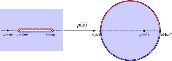
As a last warm-up it is very useful to solve this very same problem in a third way since this last approach is the closest to what we will do in higher dimensions. In this last approach to the problem we start by thinking of the S-matrix as being a function of both $s$ and $t$ as if they were independent variables; they are not since $s+t+u=4m^{2}$ and $u=0$ in two dimensions. Then $S(s,t)$ is a function with a cut for $s>4m^{2}$, another cut for $t>4m^{2}$ as well as poles for single-particle processes in the $s$- and $t$- channels. Next we use a very convenient change of variable which maps the full complex plane with those cuts removed into the unit disk. This is the map

$$s\mapsto\rho_{s}=\frac{\sqrt{4m^{2}-s_{0}}-\sqrt{4m^{2}-s}}{\sqrt{4m^{2}-s_{0}}+\sqrt{4m^{2}-s}}\,,\qquad\;\;\;\;\;s=\frac{s_{0}(1-\rho_{s})^{2}+16m^{2}\rho_{s}}{(1+\rho_{s})^{2}}\,.$$ (2)

where $s_{0}<4m^{2}$ is a free parameter that we can choose according to convenience. In the present case, it is convenient to choose $s_{0}=2m^{2}$ so that $\rho_{s}=0$ corresponds to the crossing symmetric point $s=t=2m^{2}$. A similar map is also very useful in conformal bootstrap studies [4]. It is illustrated in figure 2. The top of the cut maps to the upper boundary of the unit disk and the bottom of the cut maps to the lower boundary of the disk. The interval $\left[0,4m^{2}\right]$ maps to the interval $\rho\in\left[2\sqrt{2}-3,1\right]$ so this is where we find the poles associated to stable particles.

Figure 2: Mapping from the cut $s$-plane to the unit disk given in equation (2).

Apart from the poles corresponding to single particle exchanges, $S(\rho_{s},\rho_{t})$ is analytic for both $\rho_{s}$ and $\rho_{t}$ inside the unit disk and thus we can write

$$S(s,t)=-\frac{\hat{g}^{2}}{s-m_{b}^{2}}-\frac{\hat{g}^{2}}{t-m_{b}^{2}}+\sum_{a,b=0}^{\infty}c_{ab}\,\rho_{s}^{a}\rho_{t}^{b}$$ (3)

Crossing symmetry is guaranteed provided the coefficients of the convergent Taylor expansion are symmetric, $c_{ab}=c_{ba}$. Since we are going to evaluate the S-matrix on the constraint surface $s+t=4m^{2}$ we can simplify this ansatz further. In terms of $\rho_{s}$ and $\rho_{t}$ this constraint yields

$$\rho_{s}^{2}\rho_{t}+\rho_{t}^{2}\rho_{s}+4\rho_{s}\rho_{t}+\rho_{s}+\rho_{t}=0$$ (4)

This means the representation (3) has a big redundancy. We can always add to it polynomials in the left hand side of the constraint (4). To remove this ambiguity, we can set to zero many of constants $c_{ab}$ (in appendix B we explained in detail which $c_{ab}$ can be set to zero).

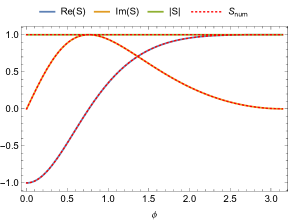
Numerically, we set a cut-off in the sum (3) and impose unitarity for $s>4$ which corresponds to the upper half circle where $\rho_{s}=e^{i\phi}$ with $\phi\in\left[0,\pi\right]$. We evaluate $|S(s,t)|^{2}$ in a uniform grid in the $\phi$ interval which gives a set of quadratic constraint equations on the $c_{ab}$ and the residues of the poles. We optimize $\hat{g}^{2}$ in the usual way using FindMaximum for example. The outcome of this third approach is in perfect agreement with our previous analytical and numerical results as illustrated in figure 3.

Figure 3: Comparison of the exact optimal S-matrix (given by $1/z(s)$ with $z$ given by (1)) to numerical results using the ansatz (3) with the $a,b$ series truncated at maximum degree $N=5$ and $m_{BS}^{2}=3$. We plot the physical region $\rho=e^{i\phi}$ with $\phi\in\left[0,\pi\right)$. The numerical results (red dashing) are indistinguishable from the exact results.

To summarize: In two dimensions we can find the optimal S-matrix with largest possible residue analytically. We do so by dividing the S-matrix by a clever guess and using the maximum modulus principle to show that this ratio should be one. We recovered the same analytic results numerically in two ways. In the first one we start from a parametrization of the kinematics where we can Taylor expand the S-matrix and then truncate that expansion to obtain a finite algebraic problem which we can put on a computer. The second numerical approach is a small variation where we think of the S-matrix as a function of $s$ and $t$ as if they were independent and then consider a double Taylor expansion in each of them.

What we implicitly used in the last method can be called an analytic extension – note that it is not an analytic continuation as we are increasing the number of variables and not just moving into the complex plane keeping the number of variables fixed. In this extension we promoted the S-matrix to a more general function of two variables which has no singularities in the cut $s$ and $t$ planes. Equivalently, in terms of the $\rho$ variables, we assumed the existence of an extension into a function $S(\rho_{s},\rho_{t})$ which has no singularities in the polydisk $\{\rho_{s},\rho_{t}\text{ such that }|\rho_{s}|\leq 1\text{ and }|\rho_{t}|\leq 1\}$ while all we know a priori is that such a regular function exists only in the intersection of the polydisk with the constraint (4). Why do we have the right to assume that such an extension exists at all? For instance, it could happen that such an extension would inevitably introduce new singularities in the full polydisk domain which would then invalidate the convergence of the double expansion (3). Numerically, using this extension method we seem to find perfect agreement with the analytic results so somehow we should be safe. Indeed, the polydisk is a so-called Stein manifold and the constraint (4) is an holomorphic embedding and as such defines a submanifold inside the polydisk which is also Stein. As discussed in greater detail below, there is a rather remarkable mathematical result which states that regular analytic extensions from Stein sub-manifolds inside Stein manifolds to the full Stein manifold do exist! The perfect numerical agreement is thus to be expected.

Of course, in two dimensions this discussion is a clear use of excessive force. On the other hand, in higher dimensions we will also make use of such analytic extensions and there we will not have the luxury of the analytic results to cross-check our numerics. The theorem alluded to above generalizes to that case as well and is key in providing confidence for the higher dimensional numerics.

There is also another more pedestrian explanation of why the double Taylor expansion numerics had to work which we present in appendix A; however, contrary to the discussion above, it makes use of particular features of the two dimensional problem and is not that useful as a warm up to the higher dimensional case.

3 Higher Dimensions

We now move on to scattering amplitudes in $d+1$ spacetime dimensions. Consider again the elastic scattering process of two identical real scalar particles of mass $m$. In our conventions the S-matrix element is

$$\langle{\bf p}_{3},{\bf p}_{4}|S|{\bf p}_{1},{\bf p}_{2}\rangle={\mathds{1}}+i(2\pi)^{d+1}\delta^{(d+1)}(p_{1}+p_{2}-p_{3}-p_{4})M(s,t,u)$$ (6)

with normalization such that

$${\mathds{1}}=(2\pi)^{2d}4E_{{\bf p}_{1}}E_{{\bf p}_{2}}\left(\delta^{(d)}({\bf p}_{1}-{\bf p}_{3})\delta^{(d)}({\bf p}_{2}-{\bf p}_{4})+(3\leftrightarrow 4)\right)$$ (7)

where $E_{{\bf p}}=\sqrt{m^{2}+{\bf p}^{2}}$. The Mandelstam invariants are given by

$$s=(p_{1}+p_{2})^{2}\qquad\qquad t=(p_{1}-p_{3})^{2}\qquad\qquad u=(p_{1}-p_{4})^{2}$$ (8)

which of course obey $s+t+u=4m^{2}$, and we henceforth work in units such that $m^{2}=1$. We often write $M(s,t)\equiv M(s,t,4-s-t)$. In the channel under consideration $s$ is the squared center-of-mass energy and the scattering angle is given by

$$x=\cos(\theta)=1+\frac{2t}{s-4}=-1-\frac{2u}{s-4}$$ (9)

Physical values of the Mandelstam invariants are therefore $4\leq s$ and $4-s\leq t\leq 0$. We can project onto channels with definite angular momentum by introducing the partial amplitudes:

$$S_{\ell}(s)=1+i\frac{(s-4)^{\frac{d-2}{2}}}{\sqrt{s}}\int\limits_{-1}^{1}\!dx\,(1-x^{2})^{\frac{d-3}{2}}P^{(d)}_{\ell}(x)\left.M(s,t)\right|_{t\to\tfrac{1}{2}(s-4)(x-1)}$$ (10)

where $P_{\ell}^{(d)}(x)$ is proportional to the Gegenbauer polynomials. In our conventions,

$$P^{(3)}_{\ell}(x)=\frac{1}{32\pi}P_{\ell}(x)\,,\qquad\qquad P^{(2)}_{\ell}(x)=\frac{1}{8\pi}\cos(\ell\theta)\ ,$$ (11)

with $P_{\ell}(x)$ the usual Legendre polynomials, normalized such that $P_{\ell}(1)=1$. We note that $S_{\ell}(s)=1$ for odd $\ell$ because Bose symmetry implies invariance under the reflection $\theta\to\pi-\theta$.

Although the S-matrix element (6) has all kind of distributional properties, the amplitude $M(s,t,u)$ is a regular function (see e.g. [6, section 4.3]). We will assume that $M(s,t,u)$ obeys three further constraints:

• Crossing Symmetry: $M(s,t,u)$ is completely symmetric in its arguments. The symmetry $u\leftrightarrow t$ follows from the aforementioned Bose symmetry, but the other generator of the crossing symmetry group can only be found from a more sophisticated analysis and requires the LSZ prescription.

• Analyticity: $M(s,t,4-s-t)$ is analytic for arbitrary complex $s$ and $t$, except for potential bound-state poles at $s=m_{b}^{2}$ with $0<m_{b}^{2}<4$, a cut along the real axis starting at $s=4$, and the images of these singularities under the crossing symmetry transformations. It further obeys the usual reality condition $M(s^{*},t^{*}4-s^{*}-t^{*})=M^{*}(s,t,4-s-t)$. We note that the analyticity assumption is actually rather optimistic, since this ‘maximal’ analyticity has not been proven from axiomatic field theory. On the other hand some a posteriori justification is provided by the remarkable agreement between some of our results and those obtained without maximal analyticity in the older literature. We therefore believe that this assumption is sufficiently mild to generate physically meaningful results. We offer some further comments on this point in section 4.4 and the conclusions section below.

• Unitarity: From $S^{\dagger}S=1$ we find that the unitarity constraint for elastic scattering takes the form

  $$\left|S_{\ell}(s)\right|\leq 1$$ (12)

  for all $s\geq 4$ and $\ell\in\{0,2,4,\ldots\}$. Generically no other channels are available for a finite window of values of $s$, starting at 4 and ending at a higher threshold (like $s=9$ for three-particle scattering). In such a window the above inequality should in fact be saturated. In this work we will not impose such saturation, but our numerics in principle allows for it.

The aim of the S-matrix bootstrap program (as we envisage it) is to use these general conditions to obtain concrete constraints on the behavior of the function $M(s,t,u)$ or the partial amplitudes $S_{\ell}(s)$ at interesting points. Many results from the previous century can be found in the textbook [10] and the reviews [11, 8].

The recent works [12, 13] pursue a bootstrap analysis of scattering amplitudes of weakly interacting higher spin theories, where the amplitudes are meromorphic functions of the Mandelstam invariants. Analytically, they beautifully explore the large $s$ and $t$ regime of weakly interacting higher spin scattering amplitudes and observe remarkable universality there. In contrast, our analysis is fully non-perturbative and the only poles of the scattering amplitudes are associated with stable particles (below the 2-particle continuum). Nevertheless it would be very interesting to investigate the same large $s$ and $t$ regime within our numerical approach.

3.1 Ansatz

In this subsection we explore the consequences of our analyticity assumption in some detail. As a toy model we can start with a single-variable function $f(z)$ which is analytic in a simple domain $D\subset\mathbb{C}$. If we define $\rho:D\to\Delta$ as a biholomorphic map between $D$ and the unit disk $\Delta=\{\rho\in\mathbb{C}\,:\,|\rho|<1\}$, then any such $f(z)$ has a Taylor series expansion of the form

$$f(z)=\sum_{n=0}^{\infty}c_{n}\rho(z)^{n}$$ (13)

which converges as long as $|\rho(z)|<1$. Our multi-variable problem is unfortunately not so easy, since for $M(s,t)$ the moving cuts imply that the domain of analyticity in one variable, say $s$, depends on the other variable $t$. We will remedy this as follows. First we relax the constraint $s+t+u=4$ and consider three-variable functions $M(s,t,u)$. Then we transform the variables $(s,t,u)\to(\rho_{s},\rho_{t},\rho_{u})$ using the map (2) which is, with $m^{2}=1$,

$$s\mapsto\rho_{s}=\frac{\sqrt{4-s_{0}}-\sqrt{4-s}}{\sqrt{4-s_{0}}+\sqrt{4-s}}\,,\qquad\;\;\;\;\;s=\frac{s_{0}(1-\rho_{s})^{2}+16\rho_{s}}{(1+\rho_{s})^{2}}\,.$$ (14)

In this case, it is convenient to choose $s_{0}=\frac{4}{3}$ so that $\rho_{s}=\rho_{t}=\rho_{u}=0$ corresponds to the crossing symmetric point $s=t=u=\frac{4}{3}$. Now, since the transformation $\rho_{s}$ maps the $s$-plane minus the right cut starting at $s=4$ to the unit disk, we see that in the $\rho$ variables all the cuts lie outside the polydisk $\Delta^{3}$ defined by $|\rho_{s}|<1$, $|\rho_{t}|<1$ and $|\rho_{u}|<1$. The only remaining singularities are then the poles and it is natural to write

$$M(s,t,u)=-\frac{g^{2}}{s-m_{b}^{2}}-\frac{g^{2}}{t-m_{b}^{2}}-\frac{g^{2}}{u-m_{b}^{2}}+\sum_{a,b,c=0}\alpha_{abc}\,\rho_{s}^{a}\rho_{t}^{b}\rho_{u}^{c}$$ (15)

where the triple $\rho$ series converges inside $\Delta^{3}$, and for definiteness we have put in the poles for a single scalar bound state of mass $m_{b}$. The demands of crossing symmetry are implemented by demanding that the coefficients $\alpha_{abc}$ are totally symmetric in their indices. When restricted to the surface defined by $s+t+u=4$ the ansatz (15) obeys the analyticity and crossing symmetry constraints. It is perhaps more surprising that the converse is also true: any function obeying the analyticity constraints on the surface $s+t+u=4$ can be extended to a function on $\Delta^{3}$, analytic modulo the poles, and therefore can be written in the form (15). This follows from a mathematical theorem known as Cartan’s theorem B, which is a statement about the vanishing of higher cohomologies of coherent analytic sheaves on Stein manifolds (see e.g. [14]) – in the case at hand this implies that there is no obstruction to an extension away from the surface $s+t+u=4$.

The triple $\rho$ expansion in equation (15) is the starting point for our numerical work. Our approach is to restrict the expansion to a finite sum by imposing

$$a+b+c\leq N_{\max}$$ (16)

and then further restricting to the constraint surface $s+t+u=4$ which is given by a polynomial equation

$$\rho_{s}^{2}\rho_{t}^{2}\rho_{u}+\rho_{s}^{2}\rho_{u}^{2}\rho_{t}+\rho_{t}^{2}\rho_{u}^{2}\rho_{s}+\text{(lower degree terms)}=0$$ (17)

and which in practice allows us to eliminate many terms in (15) (in appendix B we explain in detail which terms can be set to zero). The remaining freedom in our ansatz then consists of the finitely many remaining $\alpha_{abc}$ together with the bound state parameters; since this is a finite-dimensional space we can use a computer to numerically explore the space of scattering amplitudes. Of course we want to keep $N_{\max}$ as large as possible. As we will see, in fortunate cases the numerical results stabilize already for feasible values of $N_{\max}$, while in other cases we can extrapolate.

It will be the job of the computer to impose the unitarity constraints, which are quadratic constraints in the parameters $g^{2}$ and $\alpha_{abc}$. Rather than checking the infinity of constraints for all $s$ and $\ell$, we impose a cutoff and check that unitarity constraints are obeyed only for $\ell\leq\ell_{\max}$ and along a grid of values for $s$. Experimentally we observe that our results remain meaningful if $\ell_{\max}$ is not much smaller than $N_{\max}$ and if the grid is sufficiently refined. In appendix F we discuss the dependence on these parameters in more detail, and outline the numerical implementation.

4 Results

In this section we present our numerical results for several maximization problems using the S-matrix bootstrap method explained above. For most of this section we restrict our attention to 3+1 dimensional QFTs, i.e. $d=3$ in our notation. In the final subsection 4.4, we consider $2+1$ dimensional QFTs.

4.1 Cubic coupling

For our first result we consider a scattering amplitude with a single pole corresponding to the exchange of a scalar particle of mass $m_{b}$, exactly as in our ansatz (15), and maximize the value of the residue $g^{2}$ as a function of $m_{b}$.

Figure 4: Largest possible value $|g|_{\max}$ as a function of $m_{b}^{2}$, using a triple rho expansion of the amplitude for the given values of $N_{\max}$ and after imposing the unitarity constraints for spins up to $\ell_{\max}=20$. As explained in the text, the shaded area is physically incompatible with our analyticity assumption. We added the analytic result of appendix E as the dashed line near $m_{b}^{2}=4$.

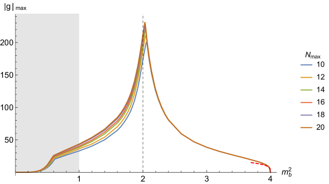
In figure 4 we plot the maximum absolute value of the coupling $|g|$ defined as the residue of the pole, with the different curves corresponding to different values of $N_{\max}$. We have obtained this plot by maximizing $|g|$ for a sequence of values of $m_{b}$ and the indicated curve is an interpolation through our data points. The plot is rather rich; we discuss its key features one by one.

• Convergence with $N_{\max}$. For $m_{b}\gtrsim\sqrt{2}$ we see that $|g|_{\max}$ is nearly stationary as we vary $N_{\max}$, whereas for $m_{b}\lesssim\sqrt{2}$ we observe more significant improvements with $N_{\max}$. We have no explanation for this disparate behaviour (although we suspect it to be related to some subtler higher energy behaviour to which our ansatz is struggling to converge – see also discussion section 5 and appendix G). Numerically we find that we can extrapolate to infinite $N_{\max}$ and appear to get a finite answer in either domain. We expect this value to correspond to an upper bound on $|g|$ for any scattering amplitude that obeys the constraints of the previous section.

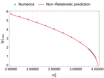
• Peak near $m_{b}\sim\sqrt{2}$. The clear peak is reminiscent of two-dimensional scattering amplitudes, where it was easily explained because in that case the $s$- and $u$-channel poles cancel precisely at $m_{b}=\sqrt{2}$ and the number $|g|$ becomes meaningless – so no upper bound can be obtained. In greater than two dimensions the cross-channel poles are smeared into a cut by the projection onto the partial waves. One can easily see from (10) that this cut starts at $s=4-m_{b}^{2}$ thus we find in the partial amplitudes the $s$-channel pole starts to overlap with the $t$- and $u$-channel cut when $m_{b}^{2}\leq 2$. While there is a singularity at the branch point of this cut with the correct sign to “screen” the $s$-channel pole, this singularity is not strong enough to fully cancel the pole as in $1+1$ dimensions. The singularity is a $\log(s-4+m_{b}^{2})$ in $3+1$ and $(s-4+m_{b}^{2})^{-1/2}$ in $2+1$ (see appendix D for the expicit expressions). We thus expect the peak in figure 4 to remain finite as $N_{\max}\to\infty$. This is borne out by some crude extrapolations (not shown).

• Behavior near threshold, $m_{b}\sim 2$. As explained in appendix E, when $m_{b}-2$ is parametrically small we can analytically constrain the behavior of $|g|_{\text{max}}$ as a function of $m_{b}$. This result is plotted in the figure as the dashed red line segment. Figure 5 shows a closer analysis of this limit. We see that it accurately traces our numerical results, with the agreement improving as $m_{b}$ approaches $2$.

• Behavior for $m_{b}<1$. In this region the scattered particle is no longer the lightest particle in the theory and on physical grounds we expect the two-particle cut in $A(s,t,u)$ to begin at $2m_{b}$ rather than at $2m$. For small enough $m_{b}$ this is corroborated by our numerics since $|g|_{\max}\sim 0$ so no pole can be present without modifying our ansatz. It would be interesting to understand in more detail the kink near $m_{b}\approx 0.5$.

Figure 5: Comparison of numerics with the non-relativistic prediction $|g|_{\text{max}}\sim 256\pi\sqrt{2-m_{b}/m}$ derived in appendix E. These numerics were performed with $s_{0}=m_{b}^{2}$ so that the bound state pole always maps to the centre of the $\rho$ disk. This greatly expedites the convergence in this limit. For example one can already see convergence with $N_{\text{max}}=2$ and $\ell_{\text{max}}=4$ which are the parameter values used for this plot.

For $m_{b}=1$ we can identify the pole with an exchange of the external particle. Reference [15] (see also [10]) discusses an analytic upper bound on $|g|$ for that case which in our conventions takes the value:

$$|g|\lesssim 16\pi\sqrt{1.5\cdot 10^{6}}\approx 61562.4$$ (18)

which is far weaker than our current bounds.

4.2 Quartic coupling

Figure 6: A first attempt at obtaining a maximal value of the quartic coupling $\lambda\equiv\frac{1}{32\pi}M(\frac{4}{3},\frac{4}{3},\frac{4}{3})$, using the ansatz (15) with $g=0$. We impose the unitarity constraint (12) for all $\ell\leq\ell_{\text{max}}$. Convergence requires larger $\ell_{\text{max}}$ for higher values of $N_{\text{max}}$. With this ansatz, the maximal quartic coupling continues to increase significantly with $N_{\text{max}}$ even for $N_{\text{max}}=20$. The black line indicates the value $2.262$ achieved in the solution of [16], while the red line indicates the rigorous upper bound $2.75$ of [17]. For large enough $\ell_{\text{max}}$ and $N_{\text{max}}$ our curves must eventually form a plateau between these two lines, however the convergence is so poor that this cannot be inferred from the plot.

Our second set of results concerns the scattering amplitudes $M(s,t,u)$ without any bound state poles, as for example would be the case in $\pi^{0}$ scattering. We will constrain the value of the amplitude at the symmetric but unphysical point $s=t=u=4/3$ and therefore define:

$$\lambda\equiv\frac{1}{32\pi}M\left(\frac{4}{3},\frac{4}{3},\frac{4}{3}\right)$$ (19)

Historically $\lambda$ was taken to be a measure of the quartic pion interaction strength. In previous works [17] it was constrained both from above and below, in our conventions:

$$-8.2\leq\lambda\leq 2.75$$ (20)

These constraints stem only from the use of axiomatially proven analyticity, crossing and unitarity. Another data point is provided by the explicit “amplitudes” constructed by Auberson and Mennessier, one with $\lambda=2.62$ [16] and one with $\lambda=-1.69$ [18], both of which obey analyticity, crossing and unitarity. This provides a lower bound for any upper bound and vice versa. It is particularly remarkable that there exists a fairly narrow interval $[2,62,2.75]$ in which the best upper bound must reside.

Figure 7: Maximal value of the quartic coupling $\lambda\equiv\frac{1}{32\pi}M(\frac{4}{3},\frac{4}{3},\frac{4}{3})$, now using the ansatz (15) with $g=0$, supplemented with the term (21). With this improved ansatz, the maximal quartic coupling effectively saturates for $N_{\text{max}}\gtrsim 6$. A few values of $\ell_{\text{max}}$ are shown to demonstrate that the value of the plateau is independent of this cutoff – the data points for various $\ell_{\text{max}}$ are indistinguishable until around $N_{\text{max}}\gtrsim 12$ where the plateau is lost for $\ell_{\text{max}}=10$ (this is just the usual loss of the plateau when $N_{\text{max}}$ becomes too large compared to $\ell_{\text{max}}$).

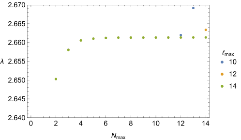
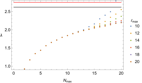
Let us first discuss the case of the upper bound. Figure 6 shows the largest possible value on $\lambda$ using the ansatz (15) (with $g=0$). One can see that the convergence with $N_{\text{max}}$ is quite slow which suggests the presence of a singularity near or on the boundary of the $\rho$ discs. Indeed, as pointed out in [17, 16] the amplitude which achieves the upper bound naturally has a singularity of the form $(s-4)^{-1/2}$ corresponding to a bound state sitting precisely at threshold. Physically this is intuitive: the positive sign of the amplitude corresponds to an attractive interaction. The situation in which the interaction is as attractive as possible without introducing new bound states occurs just at the point where a resonance is pulled all the way to the threshold. Mathematically it is natural that to make the amplitude as big as possible at the symmetric point it should be made as big as possible at threshold. Figure 7 shows the bound on $\lambda$ with the threshold bound state included in the anstaz. This amounts to adding

$$\alpha\left(\frac{1}{\rho_{s}-1}+\frac{1}{\rho_{t}-1}+\frac{1}{\rho_{u}-1}\right)$$ (21)

to the ansatz (15) where now $\alpha$ is another parameter to be varied. This singularity does not cause a violation of unitarity because it is canceled by the phase-space volume factor in (12). More precisely, we find that the $\ell=0$ partial amplitude near threshold behaves like

$$S_{0}(s)=1+\frac{1}{16\sqrt{6}\pi}\alpha+O(\sqrt{s-4})\,.$$ (22)

and therefore

$$-32\sqrt{6}\pi\leq\alpha\leq 0\,.$$ (23)

The unitarity constraints for the higher spin partial amplitudes do not lead to further restrictions on $\alpha$.

Once the threshold bound state (21) is included we find that convergence is now quite rapid as indicated by the plateau in figure 7 already seen at modest values of $\ell_{\text{max}}$ and $N_{\text{max}}$. The height of the plateau is $2.6613...$ and since

$$2.62<2.6613...<2.75.$$ (24)

it falls beautifully below the rigorous bound of [17] but above the solution constructed in [16]. Given the flexibility of our anstaz we expect this value to represent the strictest possible bound that derives from unitarity, crossing and analyticity of a single amplitude.

Figure 8: Real and imaginary parts of $S_{0}$ for $N_{\text{max}}=12$ and $\ell_{\text{max}}=20$ (left plot). Absolute value of $S_{0}$ for $\ell_{\text{max}}=20$ and several values of $N_{\text{max}}$ (right plot).

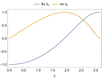
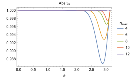
An interesting feature of the optimal solution is what appears to be a tendency toward saturation of unitarity. In right plot in figure 8 one can see that $|S_{0}|$ increasingly saturates unitarity for increasing values of $N_{\text{max}}$. A related fact is that we observe numerically $\alpha=-32\sqrt{6}\pi$ to great accuracy indicating that unitarity is saturated at threshold. Unitarity saturation is also observed in the higher partial waves.

Let us now consider the lower extremum for which our results are shown in figure 9. As in the previous case (without the threshold singularity) the convergence is quite slow in $N_{\text{max}}$. Unfortunately the addition of a threshold bound-state of the form (21) cannot save us here, since we would need $\alpha>0$ to lower the value of $\lambda$ but according to (23) this is not allowed by unitarity of the spin 0 partial amplitude at threshold. Physically this makes sense – if $\lambda<0$ then this indicates a repulsive force which does not favour the creation of bound states nor moving resonances down to the threshold value. Unfortunately we were not able to identify the relevant singularity in this case and thus were not able to improve the slow convergence.

Figure 9: Minimal value of the quartic coupling $\lambda\equiv\frac{1}{32\pi}M(\frac{4}{3},\frac{4}{3},\frac{4}{3})$ achieved with the ansatz (15) (with $g=0$). With this ansatz, the minimal quartic coupling continues to decrease significantly with $N_{\text{max}}$ even for $N_{\text{max}}=20$.

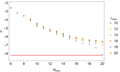
Notwithstanding these convergence issues, we did already significantly improve the lowest possible value of $-1.69$ that was explicitly constructed in [18]. As the authors of that paper already noted, the discrepancy between their $-1.69$ and the lower bound $-8.2$ of [17] means that either the lower bound is quite far from optimal, or that the behaviour of the amplitude which provides this bound is quite “wild” so as to not be contained within the space of functions they explored. Our results indicate that the latter scenario is the correct one since we do seem to be approaching a value in the ball park of the lower bound in (20).

4.3 Exploring scattering lengths

Another set of observables that received interest in days long gone were the scattering lengths $a_{\ell}$. These are defined as the behavior of the partial waves when $s$ approaches its threshold value 4. We will restrict ourselves to four spacetime dimensions, i.e. $d=3$, where it is typically defined as

$$a_{\ell}\colonequals\lim_{s\to 4}\frac{S_{\ell}(s)-1}{i(s-4)^{\ell+1/2}}\,.$$ (25)

with the limit taken from above in order to make direct contact with experiment. The power of $s-4$ in the denominator arises as follows. One assumes that $\lim_{s\to 4}M(s,t)$ is finite for all $t$ in some neighborhood of zero. Analyticity in $t$ then allows one to write down a Taylor series expansion in $t$ whose radius of convergence remains strictly positive as $s\to 4$. Substituting $t=\frac{1}{2}(s-4)(x-1)$ and doing the $x$ integral in (10) to project onto the partial waves of spin $\ell$ then gives a finite scattering length for all $\ell$ precisely with the given prefactor (recall that we are considering $d=3$). The factor of $i$ is included to make the scattering length real if $M(s,t)$ is real-analytic. In this section we will investigate constraints on the scattering length for amplitudes without bound state poles, so we will be using the ansatz (15) without the pole terms.

Let us begin with the largest possible values of the scattering length. We first recall that, in ordinary quantum mechanics, scattering lengths are known to diverge when a resonance crosses the threshold value $s=4$. In the $\rho$–variables in $d=3$ this can be seen by considering scattering amplitudes that locally take the form

$$-\mu\frac{P_{\ell}^{(3)}(x)}{\rho_{s}-1-\epsilon}+\ldots$$ (26)

with the dots denoting subleading terms, which include permutations to make the amplitude crossing symmetric and other terms to make the amplitude unitary for $s$ away from 4. From unitarity near $s=4$ we obtain the constraint

$$0\leq\mu\leq\frac{2\ell+1}{(8\pi)^{2}\sqrt{4-s_{0}}}$$ (27)

where we recall that $s_{0}$ in our ansatz is equal to $4/3$ and we used that $\int_{-1}^{1}dx\,P^{(3)}_{\ell}(x)^{2}=[512\pi^{2}(2\ell+1)]^{-1}$ in our conventions. The important observation here is that unitarity bounds $\mu$ independently of the value of $\epsilon$, whereas the contribution to the spin $\ell$ scattering length is given by

$$\frac{(16\pi)^{2}\mu}{(2\ell+1)\epsilon}$$ (28)

so by sending $\epsilon$ to zero from above we can get an infinitely large positive scattering length. Notice that $\epsilon<0$ creates a pole on the physical sheet and this is disallowed by our ansatz.

Figure 10: Exploring large values of the scattering length. We plot the largest obtained spin 0, 2 and 4 scattering lengths as a function of the number of terms in our ansatz as parametrized by $N_{\max}$. For the larger values of $N_{\max}$ we include two values of $\ell_{\max}$. The results are in line with the expectation of unbounded growth as $N_{\max}\to\infty$.

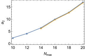
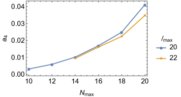
The unboundedness from above is borne out by our numerical results. In figure 10 we plot the largest possible values we can obtain for the spin 0, 2 and 4 scattering lengths with our usual ansatz (15), again with $g=0$. We observe no convergence to a finite value as we increase $N_{\max}$.

We can also consider the lowest possible values of the scattering lengths. For spin 0 the best known lower bound dates from 1980 and is given by [20]

$$a_{0}\gtrsim-1.7\,,$$ (29)

which slightly improves on a more precise bound obtained five years earlier in [21]:

$$a_{0}\geq-1.75\,.$$ (30)

These result were the culmination of a series of works, starting with the observations in [22] which were followed by a series of intermediate improvements in e.g. [10, 23, 24, 20]. Our numerical results are shown in figure 11 and are clearly converging in the neighborhood of the above lower bounds. This shows that the lower bound can more or less be saturated (with an amplitude that falls within our ansatz), which is actually a new result: the best known constructible value was -0.88 [18].

Figure 11: Lowest possible value of the scattering length as a function of $N_{\max}$. Red dashed line: precise lower bound obtained in [21]. Red shaded band: approximate lower bound obtained in [20].

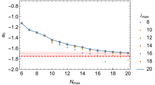
In fact, it may appear that we get dangerously close to the value $-1.7$ and that further increasing $N_{\max}$ may push us over the edge. However for this particular bound the convergence with $\ell_{\max}$ is quite slow and the value corresponding to infinite $\ell_{\max}$ may in fact increase a little bit. It would be interesting to perform a precision study with larger values of $\ell_{\max}$ and $N_{\max}$ and to simultaneously re-compute with higher precision the lower bound of $-1.7$ obtained in [20]. We leave this to the future.

For the higher spin scattering lengths one can use the Froissart-Gribov representation, see e.g. [11], to arrive at the simple lower bound:

$$a_{\ell}\geq 0\qquad\forall\ell\geq 2$$ (31)

This is borne out by our numerics but we do not show the results since a plot consisting of nothing but zeroes is not very interesting.

4.4 Bonus feature: three spacetime dimensions and QFT in AdS

In our previous work [1] we outlined another method for constraining QFT data, based on putting a QFT in AdS. The main idea is to investigate the boundary correlation functions, which behave exactly like CFT correlation functions (except there is no stress tensor) and are therefore amenable to an ordinary conformal bootstrap analysis. As we explained in [1], the translation between boundary and bulk quantities parallels the standard AdS/CFT dictionary, for example $m^{2}R^{2}=\Delta(\Delta-d)$, and furthermore we found precise formulae that dictate how the boundary correlation functions morph into flat-space scattering amplitudes upon sending the AdS curvature to zero. In [1] we numerically tested these equations in 1+1 dimensions and found a quantitative match between the two approaches to the S-matrix bootstrap.

For this paper we set out to repeat this exercise for QFTs in 2+1 dimensions. We focused on the 2+1 dimensional version of the maximal possible coupling that we discussed in section 4.1. This setup was called scenario I in [1]. We discuss the salient points of the methodology before presenting the results.

4.4.1 S-matrix bootstrap approach

For the S-matrix bootstrap, the only difference in the implementation between the 3+1 dimensional analysis of section 4.1 and the present one is that we were no longer able to compute the partial amplitudes (10) analytically. The method explained in appendix D fails because the factor $(1-x^{2})^{\frac{d-3}{2}}$ in (10) introduces an additional square-root cut in $2+1$ dimensions ($d=2$ in the conventions of this paper). Thus we are forced to evaluate the partial amplitudes by brute force use of Mathematica’s NIntegrate. Although slow, this approach is manageable with the use of multiple computing cores. This leads us to the:

• First approach: maximal three-point coupling $g^{2}$ for any flat-space QFT, obtained by assuming a flat-space scattering amplitude captured by our ansatz (15) and obeying the unitarity condition (12), as a function of $m_{b}/m$.

4.4.2 QFT in AdS approach

For the QFT in AdS approach we refer to [1] for a detailed exposition of the method, except that presently we consider two-dimensional rather than one-dimensional conformal four-point functions. This implies that there is an extra cross ratio, since $z$ is no longer kinematically equal to $\bar{z}$, and conformal blocks are labelled by a pair $(\Delta,\ell)$ rather than just the scaling dimension $\Delta$. The combined effect of these modifications is simply that the numerics is computationally much more demanding.

Now, in [1] we obtained a precise match in 1+1 dimensions by taking the raw numerical QFT in AdS results and performing a double extrapolation: first to “infinite computational power” and then to infinite $\Delta$ corresponding to the flat-space limit. For our 2+1 dimensional results we unfortunately run into trouble at the first step: our numerical results, obtained for $1\leq\Delta\leq 20$ with functionals with up to 136 components, were not amenable to reliable extrapolations. We therefore chose to present the result directly for a QFT in AdS. We chose $\Delta=17$ as a representative value. Altogether this gives the:

• Second approach: maximal three-point (bulk) coupling $g^{2}$ for a QFT in AdS, obtained by assuming boundary correlation functions consistent with unitarity and a spectrum with the natural two-particle gaps, again as a function of $m_{b}/m$.

4.4.3 Results

Figure 12: Investigating the coupling between two particles of mass $m=1$ and a third particle of mass $m_{b}$ in 2+1 dimensional QFT. First approach: maximum flat-space coupling for a QFT obtained with our ansatz (15). We plot two curves with $N_{\max}$ equal to 10 (bottom) and 18 (top) which lie almost on top of each other. Second approach: upper bound on the bulk coupling for a QFT in AdS with a radius of curvature $R\approx 16$. The four curves connect the sets of data points which were obtained with functionals with 10 (top), 36, 78 and 136 (bottom) components.

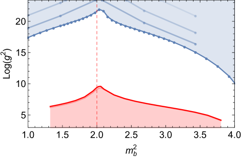
The resulting bounds are shown in figure 12. Notice the logarithmic scale. It is clear that the upper bound obtained from QFT in AdS is way larger than the largest value obtained from the S-matrix bootstrap, but the AdS results have not converged yet and one may hope that the numerical upper bound can decrease much further. The good news, however, is the remarkably similar shape of the two curves, both having a somewhat asymmetric peak slightly above $m_{b}^{2}=2$. In this sense we see a repetition of the results in 1+1 dimensions, namely that we can obtain similar bounds on the residue of a pole in a scattering amplitudes using two drastically different methods.

Physically, it is important to realize that our QFT in AdS approach is completely devoid of any assumptions about the analyticity of the flat-space scattering amplitude. If one agrees that the result in figure 12 provides evidence of the equivalence between the two approaches, then either our S-matrix bounds on the coupling do not require the amount of analyticity that we have imposed or the analyticity (at least of the extremal scattering amplitudes) is a property that we may hope to derive from the QFT in AdS construction. Either option would be very interesting and should be investigated further.

Although $\Delta=17$ was the largest value for which we had a full set of results, let us briefly discuss the result for $0<\Delta\leq 20$. In line with the results in [1], the absolute value of the numerical bounds decreases quickly upon decreasing $\Delta$. For $\Delta\gtrsim 4$ the curve always has a peak hovering around $m_{b}^{2}=2$, which broadens a bit upon decreasing $\Delta$. For $0<\Delta\lesssim 4$ the peak moves more or less linearly towards $m_{b}^{2}=4$ as $\Delta\to 0$. In the future it would be interesting to invest more computational resources and explore in more detail both this behavior and the general convergence of the bounds.

5 Discussion

Here we continued our exploration of the space of S-matrices of gapped quantum field theories initiated in [1, 2]. We present a fresh approach to an old question of constraining S-matrix elements based on unitarity, crossing and analyticity. The former two properties are firmly established properties of the S-matrix whose meaning requires no clarification. By analyticity we mean the rather simplistic (but perhaps most natural) assumption that $M(s,t,u)$ is an analytic function of each of its variables with no singularities in their respective cut planes. We make no assumption about the properties of the S-matrix outside of this union of cut planes – i.e. off the physical sheet.

Of course there are many open questions in S-matrix theory pertaining to analyticity. Are all singularities in the complex Mandelstam variables $s,t,u$ associated to Landau diagrams (as expected based on perturbation theory) or should we be open to more exotic possibilities especially in strongly coupled theories? What is the most general possible large energy behaviour of scattering amplitudes? Finally, if we bravely cross the gates and delve into the various Riemann sheets of non-perturbative scattering amplitudes by crossing its various cuts in the physical sheet, what kind of scary Chimeras await us down there?

We tried to be optimistic – by assuming the minimal expected singularities in the physical sheet – and cautious at the same time – by assuming as little as possible about the uncontrollable world of the other unphysical sheets or the large energy behaviour of scattering amplitudes. In short we mapped the physical sheet into a few unit disks and assumed little about the behaviour of amplitudes on the boundary of those disks which is where both the large energy behaviour as well as the various physical thresholds lie. Inside these disks we assumed that the only singularities were poles associated to stable bound states.

In the future, it would be interesting to develop new numerical investigations relying on more rigorous analyticity assumptions. Perhaps our results are not too sensitive to this distinction, or perhaps we will encounter exotic S-matrices which make use of the allowed non-analyticity to allow for a wider range of values. Both would be very interesting! To this end, it is worth noting that in the case of the quartic pion coupling and the lower bound on the spin zero scattering length we can say with confidence that we are in the former scenario – our results approach the bounds obtained in [17, 18] and in [20] which are based on rigorously proven analyticity properties. More evidence for the first scenario is the at least qualitative match between our maximal coupling and the upper bound on the same observable for a QFT in AdS, since the latter computation relied on no analyticity properties whatsoever. Finally we can point to the consistency of our approach with a Mandelstam representation expansion discussed in appendix C.

As for the behaviour at the boundary of the disks the idea here is that we can be agnostic about it and let regular Taylor expansions in the bulk converge towards whatever they want to. Of course, without inputing the correct singularities at the boundary of the disk, the numerics should still work but their convergence will suffer considerably. We encountered two examples of this already in the main text. The first is the quartic coupling numerics whose convergence increased substantially once we allowed for a bound state singularity at threshold. Another example is probably the four dimensional bound state coupling numerics when the bound-state mass is less than $\sqrt{2}$ times the mass of the lowest particle. The numerics are converging much slower for that range as clearly seen in the left curves in figure 4. We suspect in this case it is rather related to a non-trivial large energy behaviour of the S-matrix which the ansatz has a hard time reproducing. It would be interesting to investigate this further.

It is also at the boundary of these disks where we read physical amplitudes with any $s>4m^{2}$ and negative $t$. Multi-particle production will show up as further cuts at larger $s$ such as $9m^{2}$, $16m^{2}$, etc and infinitely many others like $(m+m^{\prime})^{2}$, etc if there are other stable particles. We saw no signs of these singularities in our numerics. As we for example show in figure 8, our optimal S-matrices do not seem to open multi-particle production cuts in any significant way. A priori this sounds very strange. How could we have no particle production of four particles from two particles if - by crossing one particle to the past - that amplitude is related to a $3\to 3$ process which obviously must exist? Indeed, it is known [26] that particle production is mandatory. It can not be strictly zero or it would lead to important contradictions. Unfortunately, the same work [26] – or any other work as far as we know – does not put a lower bound on how much particle production one must have and as such we could not reach a sharp contradiction with the numerics which by definition can never rule out an arbitrarily low particle production.

Nonetheless, absence of particle production is unphysical in spacetime dimension greater than 2. We would like to describe more realistic theories where particle production naturally arises. One way of forcing such particle production in a natural way is to study multiple S-matrix elements where we consider a system of scattering elements involving not only the lightest particle but also the next-to-lightest etc. We are currently working on this and finding some very encouraging preliminary results in two dimensions where the bounds are often significantly improved and the corresponding S-matrices do exhibit particle production and thus must correspond to genuinely non-integrable theories in contrast to our previous work [2].

The analyticity properties of scattering amplitudes of several particles of different mass are more intricate than what we considered here. The optimistic scenario is that all singularities on the physical sheet follow from Landau diagrams describing propagation of on-shell particles. This Landau analyticity is far from being rigorously established but it is a reasonable physical conjecture to start from. Even with this assumption, we will have to deal with anomalous thresholds (singularities that arise from Landau diagrams that are not on a line). A simple example is the scattering amplitude of particles of mass greater than $\sqrt{2}$ times the mass lightest particle. We plan to analyse this issue in the future, starting in 1+1 dimensions.

Appendix A $x(s)$ vs $\rho_{s},\rho_{t}$ in $1+1$ dimensions

Consider the map

$$x(s)=\frac{2-\sqrt{4-s}\sqrt{s}}{s-2}$$

which maps the full $s$-plane minus the cuts $s>4$ and $s<0$ into the unit disc $|x(s)|\leq 1$ and the map

$$\rho_{s}=\frac{2-\sqrt{4-s}}{2+\sqrt{4-s}}$$

which maps the full $s$-plane minus a single cut $s>4$ into the unit disc $|\rho_{s}|\leq 1$. An analytic function in the $s$-plane minus the cuts $s>4$ and $s<0$ – such as the S-matrix once we subtract out its known poles – can be written as

$$f(s)=\sum_{n=0}^{\infty}c_{n}\,x(s)^{n}$$ (32)

Now, we have

$$x(s)=\frac{\rho_{s}-\rho_{t}}{1-\rho_{s}\rho_{t}}\qquad\text{where}\qquad t=4-s$$ (33)

which admits a convergent expansion in powers of $\rho_{s}$ and $\rho_{t}$ provided they are both inside the unit list (and hence so is their product in the denominator). Hence the function $f(s)$ can also be cast as

$$f(s)=\sum_{n=0}^{\infty}c_{nm}\,\rho_{s}^{n}\rho_{t}^{m}\qquad\text{where}\qquad t=4-s$$ (34)

As such, our $1+1$ numerics had to work.

Appendix B Constraint surface in $\rho$-coordinates

The on-shell condition imposes

$$0=s+t+u-4m^{2}.$$ (35)

If we write this constraint in terms of the $\rho_{s},\rho_{t}$ and $\rho_{u}$ variables with arbitrary $s_{0}$ (cf. eqn. (2)) we get a somewhat lengthy expression of the form

$$0=\left(s_{0}-\frac{4}{3}m^{2}\right)\rho_{s}^{2}\,\rho_{t}^{2}\,\rho_{u}^{2}+\ldots+\left(s_{0}-\frac{4}{3}m^{2}\right).$$ (36)

Specializing to the case $s_{0}=\frac{4}{3}m^{2}$, the point $\rho_{s}=\rho_{t}=\rho_{u}=0$ satisfies the on-shell condition. Defining then the symmetrized monomials:

$$\rho^{(a,b,c)}=\rho_{s}^{a}\,\rho_{t}^{b}\,\rho_{u}^{c}+\mbox{perms}\ ,$$ (37)

the constraint equation becomes ($m=1$):

$$0 = \rho^{(1,2,2)}-4\rho^{(1,1,2)}+\rho^{(1,2,0)}+12\rho^{(1,1,1)}-4\rho^{(1,1,0)}-\rho^{(1,0,0)}.$$ (38)

We can now obtain all such constraints by multiplying this equation by other symmetrized monomials. As an example, multiplying by $\rho^{(1,0,0)}$ we get a new identity,

$$0=\rho^{(0,0,2)}+2\rho^{(0,1,1)}-4\rho^{(0,1,2)}+\rho^{(0,1,3)}+2\rho^{(0,2,2)}-12\rho^{(1,1,1)}\\ +14\rho^{(1,1,2)}-4\rho^{(1,1,3)}-8\rho^{(1,2,2)}+\rho^{(1,2,3)}+3\rho^{(2,2,2)}.$$ (39)

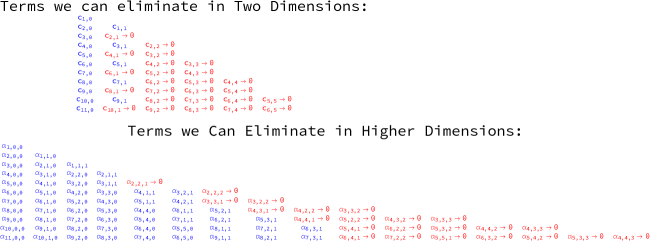
We can use these identities to systematically reduce the number of monomials in our ansatz as explained in figure 13. Note that in two spacetime dimensions we can set $u=0$ which simplifies the constraint equation to (4).

Figure 13: When centering the $\rho$ variables around general points, we can eliminate all constants $c_{a,b}$ with $a,b>1$ in two dimensions and all constants $\alpha_{a,b,c}$ with $a,b,c>1$ in higher dimensions. By centering the $\rho$ variables around $s_{0}=2$ in two dimensions and around $s_{0}=4/3$ in higher dimensions, the kinematical constraints simplify further allowing us to eliminate a few more terms in the Taylor expansions as explained in the text. An option for which terms we can eliminate is illustrated in the tables above up to $N=11$ where the level $N=a+b$ or $N=a+b+c$ is the total powers of $\rho$ in the multiple Taylor expansion. The number of terms we should keep at each level is $\frac{N}{2}+\frac{(-1)^{N}}{4}+\frac{3}{4}$ in two dimensions and $\frac{N^{2}}{12}+\frac{N}{2}+\frac{(-1)^{N}}{8}+\frac{2}{9}\cos\left(\frac{2\pi N}{3}\right)+\frac{47}{72}$ in higher dimensions.

Appendix C Mandelstam Representation

The double dispersion representation proposed by Mandelstam [28] implies that the amplitude can be written as follows

$$M(s,t,u)=B(s,t)+B(s,u)+B(t,u)\,,$$ (40)

where

$$B(s,t)=\int ds^{\prime}dt^{\prime}\frac{C(s^{\prime},t^{\prime})}{(s^{\prime}-s)(t^{\prime}-t)}\,.$$ (41)

If there are no stable particles below threshold, the double discontinuity $C(s,t)$ has support inside the region $s>4m^{2}$ and $t>4m^{2}$. In practice, this form of the double dispersion relation is not valid and one needs to include subtractions. A simple trick to derive the form of the dispersion relation with $n$ subtractions is to use the identity

$$\frac{1}{s^{\prime}-s}=\frac{(s-s_{0})^{n}}{(s^{\prime}-s)(s^{\prime}-s_{0})^{n}}+\sum_{k=0}^{n-1}\frac{(s-s_{0})^{k}}{(s^{\prime}-s_{0})^{k+1}}$$ (42)

in equation (41) for both factors in the denominator. This leads to

$$B(s,t) =(s-s_{0})^{n}(t-t_{0})^{n}\int ds^{\prime}dt^{\prime}\frac{C(s^{\prime},t^{\prime})}{(s^{\prime}-s)(t^{\prime}-t)(s^{\prime}-s_{0})^{n}(t^{\prime}-t_{0})^{n}}$$

$$+\sum_{k=0}^{n-1}(s-s_{0})^{k}(t-t_{0})^{n}\int dt^{\prime}\frac{c_{k}(t^{\prime})}{(t^{\prime}-t)(t^{\prime}-t_{0})^{n}}$$ (43)

$$+\sum_{k=0}^{n-1}(t-t_{0})^{k}(s-s_{0})^{n}\int ds^{\prime}\frac{c_{k}(s^{\prime})}{(s^{\prime}-s)(s^{\prime}-s_{0})^{n}}$$

$$+\sum_{k,l=0}^{n-1}(s-s_{0})^{k}(t-t_{0})^{l}c_{k,l}$$

where

$$c_{k}(t)=\int ds^{\prime}\frac{C(s^{\prime},t)}{(s^{\prime}-s_{0})^{k+1}}\,,\qquad c_{k,l}=\int ds^{\prime}dt^{\prime}\frac{C(s^{\prime},t^{\prime})}{(s^{\prime}-s_{0})^{k+1}(t^{\prime}-t_{0})^{l+1}}\,.$$ (44)

In general the integrals (44) do not converge. The subtracted dispersion relation is (43) considering $c_{k}(t)$ and $c_{k,l}$ as independent functions from the double discontinuity $C(s,t)$.

Stable particles correspond to delta-function pieces in the single discontinuities $c_{k}(s)$. Besides these delta-functions, the support of $c_{k}(s)$ is $s\geq 4m^{2}$. Therefore, the analytic properties of equation (43) imply that

$$B(s,t)={\rm Poles}+\sum_{a,b=0}^{\infty}\alpha_{(ab)}\rho_{s}^{a}\rho_{t}^{b}\,,$$ (45)

with a convergent double $\rho$ series in the product of two unit disks. This is a more restricted form of formula (15) where we set to zero all coefficients $\alpha_{abc}$ with $a>0$, $b>0$ and $c>0$.

In order to test the validity of Mandelstam representation, we reconsidered the problem discussed in section 4.2 using the more restricted ansatz

$$B(s,t)=\frac{\alpha}{2}\left(\frac{1}{\rho_{s}-1}+\frac{1}{\rho_{t}-1}\right)+\sum_{a,b=0}^{N_{\max}}\alpha_{(ab)}\rho_{s}^{a}\rho_{t}^{b}\,.$$ (46)

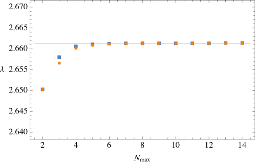
In figure 14, we show the maximal value of the quartic coupling $\lambda$ obtained with this ansatz. The maximal value $\lambda\approx 2.6613...$ is obtained for $N_{\text{max}}\gtrsim 6$. This result suggests that in the limit of large $N_{\text{max}}$ both ansatze cover the same space of functions.

Figure 14: Comparison of upper bound on pion coupling using ansatz (15) with $g=0$ and the threshold singularity $\eqref{eq:theshSing}$ included (blue squares) versus ansatz (46) (orange dots). In both cases we use $\ell_{\text{max}}=14$. The plateau converges to $2.6613...$ in both cases.

Appendix D Partial Wave Integrals

D.1 Pole contributions

Here we will consider the contribution to partial waves coming from poles of the scattering amplitude. Consider

$$M(s,t,u)_{\mbox{\tiny poles}}=-\frac{g^{2}}{s-m_{b}^{2}}-\frac{g^{2}}{t-m_{b}^{2}}-\frac{g^{2}}{u-m_{b}^{2}}.$$ (47)

It is easy to compute the partial wave decomposition of this expression. For $d=3$ we get

$$\frac{S_{\ell}(s)-1}{2i}=-\frac{g^{2}}{32\pi}\frac{\sqrt{s-4}}{\sqrt{s}}\,\left[\frac{\delta_{l,0}}{s-m_{b}^{2}}-\frac{4}{s-4m^{2}}Q_{\ell}(x_{b})\right]\,$$ (48)

with $x_{b}=x(s,t=m_{b}^{2})$ and $Q_{\ell}(z)$ the Legendre function of the second kind with branch cut along $z\in(-1,1)$. For $d=2$ we instead get

$$\frac{S_{\ell}(s)-1}{2i}=-\frac{g^{2}}{16\sqrt{s}}\left[\frac{\delta_{\ell,0}}{s-m_{b}^{2}}-\frac{2}{m_{b}\sqrt{s-4m^{2}+m_{b}^{2}}}\left(\frac{m_{b}-\sqrt{s-4m^{2}+m_{b}^{2}}}{m_{b}+\sqrt{s-4m^{2}+m_{b}^{2}}}\right)^{\!\!\ell}\ \right].$$ (49)

Now consider the contribution to the amplitude from a threshold bound state. The pole part is

$$M(s,t,u)_{\mbox{\tiny th.pole}}=-\frac{2\alpha}{\sqrt{6}\sqrt{4m^{2}-s}}-\frac{2\alpha}{\sqrt{6}\sqrt{4m^{2}-t}}-\frac{2\alpha}{\sqrt{6}\sqrt{4m^{2}-u}}.$$ (50)

If we focus on the case $d=3$, we must compute integrals of the form:

$$\int_{-1}^{1}\mathrm{d}x\frac{P_{\ell}(x)}{\sqrt{4m^{2}-t(x)}}$$ (51)

with $t(x)=-\frac{1}{2}(s-4)(1-x)$. Introducing the generating function for the Legendre polynomials

$$\sum_{n=0}^{+\infty}z^{n}P_{n}(x)=\frac{1}{\sqrt{1-2xz+z^{2}}},$$ (52)

it is not difficult to obtain

$$\int_{-1}^{1}\mathrm{d}x\frac{P_{\ell}(x)}{\sqrt{4m^{2}-t(x)}}=\frac{4}{2\ell+1}\,\frac{(\sqrt{s}-2m)^{\ell}}{(\sqrt{s}+2m)^{\ell+1}}$$ (53)

Adding up contributions from $s,t,u$ the partial amplitudes are

$$\frac{S_{\ell}(s)-1}{2i}=-\frac{\alpha}{16\sqrt{6}\pi}\frac{\sqrt{s-4m^{2}}}{\sqrt{s}}\left(\frac{i\,\delta_{\ell,0}}{\sqrt{s-4m^{2}}}+\,\frac{4}{2\ell+1}\,\frac{(\sqrt{s}-2m)^{\ell}}{(\sqrt{s}+2m)^{\ell+1}}\right)$$ (54)

D.2 $\rho_{s}\,\rho_{t}\,\rho_{u}$ contributions

Here we will show how to obtain the contribution to the partial amplitudes from terms of the form $\rho_{s}^{a}\,\rho_{t}^{b}\,\rho_{u}^{c}$ analytically in $d=3$. While the calculation is somewhat tedious, the underlying concept is simple: the integral that we want to do has only one cut (of square-root type) in the integrand and thus with a simple trigonometric change of variables the integrand can be converted to a rational function and computed by partial fractions (or some more clever method).

The non-trivial integrals to perform take the form

$$I^{\ell}_{\ b,c}=\int_{-1}^{1}\mathrm{d}xP_{\ell}(x)\,\rho(t)^{b}\rho(u)^{c}$$ (55)

with, as in (2) with $m=1$,

$$\rho(s)=\frac{1-\sqrt{1-\frac{s-s_{0}}{4-s_{0}}}}{1+\sqrt{1-\frac{s-s_{0}}{4-s_{0}}}}$$ (56)

In applications we typically set $s_{0}=4/3$. We next introduce our first inspired change of variables from $x$ to $\phi$ which is given by

$$x=-\frac{s+4}{s-4}\,\cos(2\phi).$$ (57)

In these variables we get:

$$I^{\ell}_{\ b,c}=4\,\left(\frac{s+4}{s-4}\right)\,\,\int\mathrm{d}\phi\,P_{\ell}(x(\phi))\sin(\phi)\cos(\phi)\left(\frac{1-r\cos\phi}{1+r\cos\phi}\right)^{b}\,\left(\frac{1-r\sin\phi}{1+r\sin\phi}\right)^{c}$$ (58)

where we also introduced

$$r^{2}\equiv\frac{4+s}{4-s_{0}}\,.$$ (59)

We should now do the usual change of variables,

$$\phi=2\,\arctan(y)$$ (60)

This gives

$$I^{\ell}_{\ b,c}=\frac{4^{2}r^{2}}{r^{2}-\frac{8}{4-s_{0}}}\,\int\mathrm{d}y\,P_{\ell}(x(y))\,\frac{y(1-y^{2})}{(1+y^{2})^{3}}\,\left(\frac{(1-r)+y^{2}(1+r)}{(1+r)+y^{2}(1-r)}\right)^{b}\,\left(\frac{1-2r\,y+y^{2}}{1+2r\,y+y^{2}}\right)^{c}.$$ (61)

We have

$$x(y)=\frac{r^{2}}{r^{2}-\frac{8}{4-s_{0}}}\,\frac{1-6y^{2}+y^{4}}{(1+y^{2})^{2}},$$ (62)

and the integral runs from $y_{i}$ to $y_{f}$ with

$$y_{i}=\frac{\sqrt{4-s_{0}}}{2}\,\left(r-\sqrt{r^{2}-\frac{4}{4-s_{0}}}\right),\qquad y_{f}=\left(\frac{r-\frac{2}{\sqrt{4-s_{0}}}}{r+\frac{2}{\sqrt{4-s_{0}}}}\right)^{\frac{1}{2}}.$$ (63)

The trick now is to rewrite the integration region using the discontinuity of a logarithm,

$$\int_{y_{1}}^{y_{2}}\mathrm{d}yf(y)=\frac{1}{2\pi i}\int_{y_{1}}^{y_{2}}\mathrm{d}yf(y)\,\mbox{Disc}\log\left(\frac{y-y_{2}}{y-y_{1}}\right)=\frac{1}{2\pi i}\int_{(y_{1},y_{2})}\mathrm{d}yf(y)\,\log\left(\frac{y-y_{2}}{y-y_{1}}\right)$$ (64)

where $(y_{1},y_{2})$ is a clockwise contour wrapping the line segment from $y_{1}$ to $y_{2}$. In our case $f(y)$ is a rational function, therefore we can pull the contour to infinity so that it picks up the poles of $f(y)$ to obtain exact expressions.

D.3 Large energy

Let us consider the large energy limit $s\to\infty$ of our ansatz. Since unitarity is imposed for each spin $\ell$, we are interested in the limit $s\to\infty$ with fixed scattering angle $\theta$. In this limit, we find

$$\rho_{s}^{a}\rho_{t}^{b}\rho_{u}^{c} =(-1)^{a+b+c}\left[1+\frac{2\sqrt{4-s_{0}}}{\sqrt{s}}\left(ia-\frac{\sqrt{2}b}{\sqrt{1-x}}-\frac{\sqrt{2}c}{\sqrt{1+x}}\right)\right.$$

$$\left.-\frac{4\sqrt{2}(4-s_{0})a}{s}\left(\frac{ib}{\sqrt{1-x}}+\frac{ic}{\sqrt{1+x}}+{\rm real}\right)+O\left(s^{-\frac{3}{2}}\right)\right]\,.$$ (65)

The contribution from the pole terms in our ansatz are real and of order $1/s$ in this limit and therefore can be neglected. The leading term in (65) only contributes to the spin 0 partial wave. The large $s$ expansion of $S_{0}(s)$ is given by

$$S_{0}(s)=1+\frac{is^{\frac{d-3}{2}}}{2^{2d-1}\pi^{\frac{d}{2}-1}\Gamma\left(\frac{d}{2}\right)}\sum_{a,b,c}\alpha_{abc}(-1)^{a+b+c}\left[1+\frac{2ia\sqrt{4-s_{0}}+{\rm real}}{\sqrt{s}}+O\left(\frac{1}{s}\right)\right]\,.$$ (66)

Unitarity implies that (for $d>4$ the inequality must be saturated)

$$\sum_{a,b,c}\alpha_{abc}(-1)^{a+b+c}a\geq 0\,.$$ (67)

If $d>2$ then unitarity also implies that

$$\sum_{a,b,c}\alpha_{abc}(-1)^{a+b+c}=0\,.$$ (68)

For $d=2$, the correct condition is

$$32\sqrt{4-s_{0}}\sum_{a,b,c}\alpha_{abc}(-1)^{a+b+c}a\geq\left[\sum_{a,b,c}\alpha_{abc}(-1)^{a+b+c}\right]^{2}\,.$$ (69)

For $\ell>0$ (even) we find

$$S_{\ell}(s)=1-is^{\frac{d-4}{2}}I_{\ell}\sum_{a,b,c}\alpha_{abc}(-1)^{a+b+c}a\left[1+\frac{i2\sqrt{4-s_{0}}b+{\rm real}}{\sqrt{s}}+O\left(\frac{1}{s}\right)\right]\,,$$ (70)

where

$$I_{\ell}=4\sqrt{2}\sqrt{4-s_{0}}\int_{-1}^{1}dx(1-x^{2})^{\frac{d-3}{2}}P_{\ell}^{(d)}(x)\frac{1}{\sqrt{1+x}}>0\,.$$ (71)

Therefore, unitarity implies (for $d>5$ the inequality must be saturated)

$$\sum_{a,b,c}\alpha_{abc}(-1)^{a+b+c}ab\leq 0\,.$$ (72)

For $d>3$ unitarity also implies

$$\sum_{a,b,c}\alpha_{abc}(-1)^{a+b+c}a=0\,.$$ (73)

For $d=3$ we find

$$40\pi\sum_{a,b,c}\alpha_{abc}(-1)^{a+b+c}ab\leq-\left[\sum_{a,b,c}\alpha_{abc}(-1)^{a+b+c}a\right]^{2}\,.$$ (74)

where we used that $I_{\ell}<I_{2}=\frac{\sqrt{4-s_{0}}}{10\pi}$ for $\ell>2$.

Where applicable, we have verified the above constraints a posteriori for our numerical solutions and found them satisfied to very good numerical accuracy.

As a final comment, we remark that the unitarity constraints dictate that $\lim_{s\to\infty}S_{\ell}(s)=1$ for any amplitude within our ansatz with finite $N_{\max}$. This property is likely to be too restrictive, and it is therefore worthwhile to try to improve our ansatz with more singular terms compatible with unitarity and analyticity. As a first attempt we added an extra term of the form $(\rho_{s}+1)(\rho_{t}+1)^{-1}$ plus $s$, $t$, $u$ permutations, which allows $\lim_{s\to\infty}(S_{\ell}(s)-1)$ to be non-zero – this modification however did not significantly change any of the results displayed above. In the future we plan to add other more singular terms and investigate their effect in more detail. Finally, the restricted behavior at large $s$ might also be a source of slow convergence when $N_{\rm max}\to\infty$ we have observed in some cases. This idea is also corroborated by the two dimensional analysis in appendix G.

D.4 Large spin

The partial waves can also be written in terms of an hypergeometric function,

$$P^{(d)}_{\ell}(x)=\frac{2^{1-2d}\pi^{\frac{1}{2}-\frac{d}{2}}}{\Gamma\left(\frac{d-1}{2}\right)}\,_{2}F_{1}\left(-\ell,d+\ell-2;\frac{d-1}{2};\frac{1-x}{2}\right)\,.$$ (75)

It is convenient to define

$$Q^{(d)}_{\ell}(x)=-\frac{\Gamma(l+1)(x-1)^{2-d-\ell}}{\pi^{\frac{d}{2}-1}2^{2d+\ell-1}\Gamma\left(\frac{d}{2}+\ell\right)}\,_{2}F_{1}\left(d+\ell-2,\frac{d+2\ell-1}{2};d+2\ell-1;\frac{2}{1-x}\right)$$ (76)

such that

$${\rm Disc}\left[(x^{2}-1)^{\frac{d-3}{2}}Q^{(d)}_{\ell}(x)\right]=2\pi i(1-x^{2})^{\frac{d-3}{2}}P^{(d)}_{\ell}(x)\,,\qquad-1<x<1\,.$$ (77)

Notice that for integer $d$ the function $Q^{(d)}_{\ell}(x)$ has no monodromy around $x=\infty$. We will work in the sheet where $Q^{(d)}_{\ell}(x)$ only has a branch cut from $x=-1$ to $x=1$. The factor $(x^{2}-1)^{\frac{d-3}{2}}=x^{d-3}(1-x^{-2})^{\frac{d-3}{2}}$ has the same analytic properties. Then we can write

$$\int\limits_{-1}^{1}\!dx\,(1-x^{2})^{\frac{d-3}{2}}P^{(d)}_{\ell}(x)M(s,x)=\frac{1}{2\pi i}\oint_{C}dx(x^{2}-1)^{\frac{d-3}{2}}Q^{(d)}_{\ell}(x)M(s,x)\,,$$ (78)

where the contour $C$ encircles the real segment $[-1,1]$ clockwise and $M(s,x)$ denotes the amplitude $\left.M(s,t)\right|_{t\to\tfrac{1}{2}(s-4)(x-1)}$. Since

$$Q^{(d)}_{\ell}(x)\approx-\frac{1}{2^{\frac{3d}{2}}\pi^{\frac{d-2}{2}}\ell^{\frac{d-2}{2}}\left(x^{2}-1\right)^{\frac{d-2}{4}}}\frac{1}{(x+\sqrt{x^{2}-1})^{\ell+\frac{d-2}{2}}}\,,$$ (79)

for large $\ell$ and $x^{2}>1$, we can expand the contour and drop the contribution from infinity. At large spin, the integral will be dominated by the singularity of $M(s,x)$ closer to the origin $x=0$. Generically, this will come from the poles associated with stable particles. More precisely,

$$\int\limits_{-1}^{1}\!dx\,(1-x^{2})^{\frac{d-3}{2}}P^{(d)}_{\ell}(x)M(s,x)=\frac{1}{2\pi i}\oint_{C}dx(x^{2}-1)^{\frac{d-3}{2}}Q^{(d)}_{\ell}(x)M(s,x)$$ (80)

$$=-\frac{1}{2\pi i}\left[\int_{-\infty}^{-x_{1}(s)}dx+\int_{x_{1}(s)}^{\infty}dx\right](x^{2}-1)^{\frac{d-3}{2}}Q^{(d)}_{\ell}(x)\left[M(s,x+i\epsilon)-M(s,x-i\epsilon)\right]$$ (81)

$$=-\frac{1}{i\pi}\int_{x_{1}(s)}^{\infty}dx(x^{2}-1)^{\frac{d-3}{2}}Q^{(d)}_{\ell}(x)\left[M(s,x+i\epsilon)-M(s,x-i\epsilon)\right]$$ (82)

where $x_{1}(s)$ is determined from

$$t(s,x)=m_{1}^{2}\qquad\Rightarrow\qquad x_{1}(s)=1+\frac{2m_{1}^{2}}{s-4m^{2}}\,.$$ (83)

In fact, the pole $\frac{-g^{2}}{t-m_{1}^{2}}$ contributes

$$\int\limits_{-1}^{1}\!dx\,(1-x^{2})^{\frac{d-3}{2}}P^{(d)}_{\ell}(x)M(s,x)\approx-\frac{2g^{2}}{s-4m^{2}}(x_{1}(s)^{2}-1)^{\frac{d-3}{2}}Q^{(d)}_{\ell}(x_{1}(s))\,,$$ (84)

which decays exponentially with $l$. Notice that this gives a purely imaginary contribution to $S_{\ell}(s)$ (see equation (10)), which by itself would violate unitarity. However, unitarity can be restored with a small real contribution of the order of the square of (84). At large $l$, this requires that we match the exponential behaviour

$$\left(x_{1}(s)+\sqrt{x_{1}(s)^{2}-1}\right)^{2}=x_{2}(s)+\sqrt{x_{2}(s)^{2}-1}\qquad\Leftrightarrow\qquad\frac{m_{2}^{2}}{4m_{1}^{2}}=1+\frac{m_{1}^{2}}{s-4m^{2}}\,.$$ (85)

In other words, unitarity can be restored with another particle or particles of total invariant mass squared $m_{2}^{2}\geq 4m_{1}^{2}$. This is what happens in perturbation theory where the box diagram restores unitarity of the tree-level exchanges.

Let us now study the contribution from the polynomial terms $\rho_{s}^{a}\rho_{t}^{b}\rho_{u}^{c}$ in our ansatz. The discontinuity of $M$ for $x>1$ comes from

$$\rho(t(s,x+i\epsilon))^{b}-\rho(t(s,x-i\epsilon))^{b}\approx 2ib\sqrt{\frac{2s-8m^{2}}{4m^{2}-s_{0}}}\sqrt{x-x_{\star}(s)}$$ (86)

where

$$x_{\star}(s)=\frac{s+4m^{2}}{s-4m^{2}}$$ (87)

and we only kept the leading behaviour of the discontinuity near its lower end $x_{\star}(s)$. Similarly, we can approximate

$$Q^{(d)}_{\ell}(x)\approx Q^{(d)}_{\ell}(x_{\star}(s))\exp\left[{-\ell\frac{s-4m^{2}}{4m\sqrt{s}}(x-x_{\star}(s))}\right]$$ (88)

and find

$$\int\limits_{-1}^{1}\!dx\,(1-x^{2})^{\frac{d-3}{2}}P^{(d)}_{\ell}(x)\rho_{s}^{a}\rho_{t}^{b}\rho_{u}^{c}\approx-\frac{1}{i\pi}\rho_{s}^{a}\rho_{-s}^{c}(x_{\star}(s)^{2}-1)^{\frac{d-3}{2}}Q^{(d)}_{\ell}(x_{\star}(s))\times$$ (89)

$$\times\int_{x_{\star}(s)}^{\infty}dx\exp\left[{-\ell\frac{s-4m^{2}}{4m\sqrt{s}}(x-x_{\star}(s))}\right]2ib\sqrt{\frac{2s-8m^{2}}{4m^{2}-s_{0}}}\sqrt{x-x_{\star}(s)}$$ (90)

$$= -\frac{b}{\sqrt{\pi}\ell^{\frac{3}{2}}}\frac{8m^{\frac{3}{2}}s^{\frac{3}{4}}}{s-4m^{2}}\sqrt{\frac{2}{4m^{2}-s_{0}}}\rho_{s}^{a}\rho_{-s}^{c}(x_{\star}(s)^{2}-1)^{\frac{d-3}{2}}Q^{(d)}_{\ell}(x_{\star}(s))$$ (91)

$$\approx \frac{F(s)}{\ell^{\frac{d+1}{2}}\left(x_{\star}(s)+\sqrt{x_{\star}^{2}(s)-1}\right)^{\ell}}\,b\rho_{s}^{a}\rho_{-s}^{c}$$ (92)

where $F(s)>0$ for $s>4m^{2}$. Notice that at large $\ell$ the leading contribution comes from $t\approx 4m^{2}$ which implies that $\rho_{u}\to\rho_{-s}$. Unitary implies ${\rm Re}\,S_{\ell}(s)\leq 1$ which at large $\ell$ becomes

$$\sum_{a,b,c}\alpha_{abc}\,b\left({\rm Im}\,\rho_{s}^{a}\right)\rho_{-s}^{c}\geq 0\,.$$ (93)

Notice that this condition is independent of the spin $\ell$ and of the spacetime dimension $d$. This justifies our numerical procedure of truncating the unitarity conditions at some value of the spin $\ell_{\rm max}\gg 1$. Writing $\rho_{s}=e^{i\phi}$ with $\phi\in[0,\pi]$, equation (93) can be written as

$$\sum_{a,b,c}\alpha_{abc}\,(-1)^{c}b\sin(a\phi)\left[\frac{\sqrt{1+y_{0}\cos\frac{\phi}{2}}-\cos\frac{\phi}{2}}{\sqrt{1+y_{0}\cos\frac{\phi}{2}}+\cos\frac{\phi}{2}}\right]^{c}\geq 0\,,\qquad\forall\,\phi\in[0,\pi]\,,$$ (94)

where $y_{0}=\frac{4m^{2}+s_{0}}{4m^{2}-s_{0}}>-1$.

The constraints (93) are linear constraints on the numerical coefficients and can easily be taken into account in our numerical code (again by sampling for a discrete set of values of $s$). We have run several of our analyses both with and without this additional constraint. As expected, the effect of the additional term decreases with the maximum spin $\ell_{\max}$ for which we manifestly check the unitarity constraints. For the values $\ell_{\max}$ used in our plots the effect of including (93) is always small and amounts to maybe to a one percent change in the final result.

D.5 Threshold Expansion and Elastic Unitarity

Here we shall discuss the threshold behaviour of amplitudes satisfying our ansatz. We start with the expression for the amplitude,

$$M(s,t,u)=\sum_{a,b,c=0}^{+\infty}\alpha_{abc}\,\rho_{s}^{a}\rho_{t}^{b}\rho_{u}^{c}+\mbox{poles}$$ (95)

At threshold the poles become constants and are irrelevant. This is not so for threshold poles which are discussed separately below. Define $w:=\sqrt{s-4}$. Then for $s\to 4^{+}$ above the cut we have

$$\rho_{s} = 1+2\sum_{n=1}^{+\infty}\left(\frac{i}{\sqrt{4-s_{0}}}\right)^{n}w^{n}=1+\frac{2i}{\sqrt{4-s_{0}}}w+\ldots$$ (96a)

$$\rho_{t}^{b}\rho_{u}^{c} = \sum_{k=0}^{\infty}w^{2k}\left(\sum_{n+m=k}c_{n,m}(1-x)^{n}(1+x)^{m}\right)$$ (96b)

Recall that in our conventions the partial waves take the form:

$$S_{\ell}(s)=1+i\frac{(s-4)^{\frac{d-2}{2}}}{\sqrt{s}}\int\limits_{-1}^{1}\!dx\,(1-x^{2})^{\frac{d-3}{2}}P^{(d)}_{\ell}(x)\left.M(s,t)\right|_{t\to\tfrac{1}{2}(s-4)(x-1)}.$$ (97)

The leading contribution for the spin $\ell$ partial wave corresponds to the $k=\ell$ term in the above, leading to

$$S_{\ell}(s) =1-b_{\ell}w^{d-1+2\ell}+ia_{\ell}w^{d-2+2\ell}+\ldots,$$ (98)

with real $a_{\ell},b_{\ell}$. These are linear combinations of the coefficients $\alpha_{abc}$ in our ansatz. Unitarity near threshold imposes:

$$b_{\ell} \geq 0, d\geq 2,\ell\geq 0;$$ (99a)

$$a_{0} =0, d=2,\ell=0;$$ (99b)

$$b_{0} \geq a_{0}^{2}/2, d=3,\ell=0.$$ (99c)

Near threshold we have the expansion of $S_{\ell}(s)$ in terms of the phase shift,

$$S_{\ell}(s)=e^{2i\delta_{\ell}(s)}\sim 1+2i\delta_{\ell}(s)-2\delta_{\ell}(s)^{2}+\ldots.$$ (100)

Absence of particle production would imply reality of $\delta_{\ell}(s)$, and hence a measure of the inelasticity of the amplitude at the threshold is

$$\frac{\mbox{Re}\,[1-S_{l}(s)]}{\left[\mbox{Im}\,S_{\ell}(s)\right]^{2}}=O[(s-4)^{-\ell}].$$ (101)

We see that for positive spin we generically get a divergent result in the threshold limit. This means that our ansatz does not automatically give an amplitude which becomes purely elastic as we approach threshold, unlike what we would expect on physical grounds. In order for purely elastic scattering to hold, we would have had to impose order $\ell$ linear constraints on the coefficients of the threshold expansion of the spin $\ell$ partial wave. We did not impose these in our numerical computations. However, experimentally we do find that as the number of parameters in our ansatz is increased, the coefficients in the threshold expansion seem to decrease.

Appendix E Non-Relativistic Limit

Consider a scalar $\phi$ of mass $m$ interacting with itself via the exchange of a second heavy scalar $\Phi$ with mass $m_{b}=2m-\epsilon$ with small $\epsilon$. We can think of $\Phi$ as a loosely bound state of two $\phi$ particles with binding energy $\epsilon$. The two body amplitude for $\phi+\phi$ scattering contains a pole at $s=m_{b}^{2}$ due to virtual production of a $\Phi$ which is just below the the two-particle threshold at $s=(2m)^{2}$. The residue of this pole $g^{2}$ is the square of the $\phi\phi\Phi$ coupling. Now consider low energy $\phi+\phi$ scattering and write $s=(2m+E)^{2}$ where $E$ is the centre of mass energy after subtraction of the rest mass. The $s$-channel pole of the amplitude is given by

$$M^{\text{pole}}=\frac{m^{5-d}g^{2}}{s-m_{b}^{2}}\sim\frac{m^{5-d}g^{2}/\epsilon}{4m(E/\epsilon+1)}$$ (102)

where we have assumed small $E$ and $\epsilon$. The $l=0$ phase shift inherits this pole through the relation

$$\,\frac{\sqrt{s}}{i(s-4m^{2})^{\frac{d-2}{2}}}(S_{0}(s)-1)=\int\limits_{-1}^{1}\!dx\,(1-x^{2})^{\frac{d-3}{2}}P^{(d)}_{0}(x)\left.M(s,t)\right|_{t\to\tfrac{1}{2}(s-4)(x-1)}$$ (103)

Plugging (102) into (103) and zooming in on the pole of the phase shift at $s=(2m-\epsilon)^{2}$ we have

$$2^{3-d}m(m\epsilon)^{1-d/2}S^{\text{pole}}_{0}(E/\epsilon)\sim\frac{2^{1-2d}\pi^{1-\frac{d}{2}}}{\Gamma\left(\frac{d}{2}\right)}\frac{m^{5-d}g^{2}/\epsilon}{4m(E/\epsilon+1)}$$ (104)

We write the pole of the phase shift as $g_{NR}^{2}/(E/\epsilon+1)$ where $g_{NR}^{2}$ is the residue in units of the binding energy $\epsilon$. We then have

$$g^{2}\to\,2^{4+d}\pi^{\frac{d}{2}-1}\Gamma(d/2)g_{NR}^{2}(\epsilon/m)^{2-\frac{d}{2}}$$ (105)

We will show below that there is a bound on the non-relativistic coupling $g_{NR}^{2}\leq 2^{2}$. Note that this correctly predicts the behaviour

$$g^{2}_{1+1}\leq 2^{7}(\epsilon/m)^{3/2}$$ (106)

in $1+1$ dimensions [2]. Moreover, this limit has been studied extensively in $3+1$ dimensions ($d=3$) [29, 30]. These authors find (adding a factor of 2 to their results to account for identical particles)

$$g_{3+1}^{2}\leq 2^{8}\pi\sqrt{\epsilon/m}$$ (107)

and thus we find perfect agreement with (105).

Let us now derive the bound on $g_{NR}^{2}$ quoted above. Recall that we are considering a very weakly bound state with binding energy $\epsilon$. We wish to obtain the behaviour of $g_{\text{max}}^{2}(\epsilon/m)$ for small $\epsilon/m$. Thus we concentrate on “slow” physics at energies $E\sim\epsilon$ (recall $E$ is the centre of mass energy after removal of the rest mass). Formally, in the phase shift we consider $s\to\bar{s}\epsilon^{2}$ and consider finite $\bar{s}$ as $\epsilon\to 0$. Any singularites of the phase shift that are a finite distance (in $s$) from the two-particle threshold – e.g. the left cut and inelastic thresholds – will be infinitely far away in $\bar{s}$ and thus only contribute through positive powers of $\epsilon$. We can thus neglect these singularities to obtain the leading behaviour of $g_{\text{max}}^{2}(\epsilon/m)$ and consider a non-relativistic phase shift $S_{\text{NR}}(\bar{E})$ with only a right-hand cut starting at $\bar{E}=0$ and a single bound-state pole at $\bar{E}=-1$, where $\bar{E}=E/\epsilon$. Since this phase shift is bounded by unitarity along the cut and cannot grow faster than a constant at infinity then the residue of the pole can easily be bounded by maximum modulus theorem. Perhaps the cleanest way to derive the precise value of the bound is to consider the change of coordinates

$$x(E)=\frac{1-(-\bar{E})^{1/2}}{1+(-\bar{E})^{1/2}},\;\;\;\;\;\bar{E}(x)=-\frac{(x-1)^{2}}{(x+1)^{2}}$$ (108)

which maps the E-plane minus the positive real axis to the unit disk and maps the bound state pole to the origin

$$\frac{g_{NR}^{2}}{\bar{E}(x)-1}\sim\frac{g^{2}_{NR}}{4\,x}$$ (109)

Now note that the function $f(x)=x\,S_{\text{NR}}(x)$ is analytic throughout the unit disk and obeys $|f|\leq 1$ on the boundary due to unitarity. Thus maximum modulus theorem implies $1\geq f(0)=g_{NR}^{2}/4$ which is the desired bound.

Appendix F Semidefinite programming implementation

Consider an ansatz as in (15), truncated such that $a+b+c\leq N_{\max}$. After eliminating the redundant monomials as described in appendix B, we are left with a finite subset of the $\alpha_{abc}$, which together with the coupling $g^{2}$ completely determine the amplitude. Let us group these real coefficients into a vector that we call $\vec{\eta}$, so we can schematically write (15) as

$$M(s,t,4-s-t)=\vec{\eta}\cdot\overrightarrow{M(s,t)}$$ (110)

with $\overrightarrow{M(s,t)}$ the vector of functions of $s$ and $t$ that each coefficient multiplies. We then substitute into the partial amplitude projection (10) and get, schematically,

$$S_{\ell}(s)=1+i\vec{\eta}\cdot\overrightarrow{f_{\ell}(s)}$$ (111)

with $\overrightarrow{f_{\ell}(s)}$ defined in the obvious way as the integral of $\overrightarrow{M(s,t)}$ against the Gegenbauer polynomials with the right prefactor. The unitarity constraints $|S_{\ell}(s)|^{2}\leq 1$ now dictate that for all physical $\ell$ and $s$ we must have

$$\left(1-\vec{\eta}\cdot\vec{I}\right)^{2}+(\vec{\eta}\cdot\vec{R})^{2}\leq 1\qquad\Leftrightarrow\qquad U\equiv 2\vec{\eta}\cdot\vec{I}-(\vec{\eta}\cdot\vec{I})^{2}-(\vec{\eta}\cdot\vec{R})^{2}\geq 0$$ (112)

with $\vec{R}=\text{Re}[\overrightarrow{f_{\ell}(s)}]$ and $\vec{I}=\text{Im}[\overrightarrow{f_{\ell}(s)}]$. This constraint can be re-phrased as a semidefiniteness condition. Indeed, consider the matrix

$$M:=\left(\begin{array}[]{cc}1+\vec{\eta}\cdot\vec{R}&1-\vec{\eta}\cdot{\vec{I}}\\ 1-\vec{\eta}\cdot{\vec{I}}&1-\vec{\eta}\cdot\vec{R}\end{array}\right)$$ (115)

The eigenvalues of this matrix are precisely

$$\lambda_{\pm}=1\pm\sqrt{1-U}$$ (116)

As befits a Hermitian matrix, they are always real since $U\leq 1$ by construction. It is now clear that

$$M\succeq 0\Leftrightarrow U\geq 0.$$ (117)

and the unitarity constraints are therefore precisely those of a semidefinite program.

We need to choose a grid of values of $s$ and a finite set of spins $\ell$ for which to test the unitarity constraints. We found it sufficient to take approximately 200 values of $s$, interspersed uniformly along the upper half of the unit circle in the $\rho_{s}$ variable defined in the main text. We observed no significant change in the results by taking a more refined $s$ grid, or by distributing the points differently along the unit circle. The maximal value of the spin $\ell_{\max}$ is indicated in the various plots. Notice that $\ell_{\max}$ needs to be sufficiently big since otherwise the extremal value completely destabilizes – see for example the data points in figure 6 with $\ell_{\max}=10$ for large $N_{\max}$. In practice we observed convergence by taking $\ell_{\max}$ at least as large as $N_{\max}$, and for the scattering length computations we needed at least $N_{\max}+4$. Increasing $\ell_{\max}$ beyond these values did not affect our results.

In our numerical computations we did find it necessary to retain very high precision, generally at least 1000 binary digits. This appears to stem from the approximate redundancy that remains even after imposing the polynomial constraint B. To illustrate this we can for example compute a derivative like

$$\begin{split}&\frac{\partial^{2}}{\partial s^{2}}\left.\left(\sum_{a,b,c}\alpha_{abc}\rho^{a}(s)\rho^{b}(t)\rho^{c}(4-s-t)\right)\right|_{s=t=4/3}=\\ &\qquad\frac{9}{256}\left(\alpha_{100}+\alpha_{001}+\frac{1}{2}\alpha_{200}+\frac{1}{2}\alpha_{002}-\frac{1}{2}\alpha_{101}\right)\end{split}$$ (118)

In a typical solution we find that this derivative is rather modest in magnitude, of order $10^{2}$ or so, whereas the individual coefficients can be very large, of order $10^{24}$ in some solutions. These kind of cancellations require high precision.

We have performed all the numerical computations in section 4 with sdpb [31]. Details of the computations like parameter settings are available from the authors upon request.

Appendix G Slow convergence on a simple 2D example

In this appendix we revisit once more the two dimensional problem considered in section 2 but this time done in the language of the $M$ amplitude rather than $S$. In two dimensions the two are simply related by

$$S(s,t)-1=\frac{1}{2\sqrt{st}}\times M(s,t)\,,\qquad s+t=4m^{2}\,.$$ (119)

and unitarity then reads

$$\text{Im}(M(s,t))-\frac{1}{4\sqrt{-st}}|M(s,t)|^{2}\leq 0\qquad\text{for}\qquad s=4m^{2}-t>4m^{2}\,.$$ (120)

This discussion will provide us with a simple example of numerics which work yet converge very slowly until we slightly improve our ansatz and thus completely solve this convergence issue.

Figure 15: Plot of $|(S_{\text{num}}-S_{\text{analytic}})/S_{\text{analytic}}|$, that is of the relative mismatch in the numerical solution in this two dimensional example where the analytic solution is available. In all these plots we use $\Lambda=20$ and check unitarity in a small grid of $40$ points. With these parameters, mathematica’s built-in FindMaximum suffices and produces an outcome in about two or three seconds. We see on the left that for $m_{b}>\sqrt{2}m$ the agreement is spectacular with the most naive ansatz (122) while in the middle we see that the agreement is much worse (a few percent off) with the same ansatz when $m_{b}<\sqrt{2}m$. On the right we see that this is neatly fixed - leading again to a perfect convergence - by simply adopting an improved ansatz as in (123).

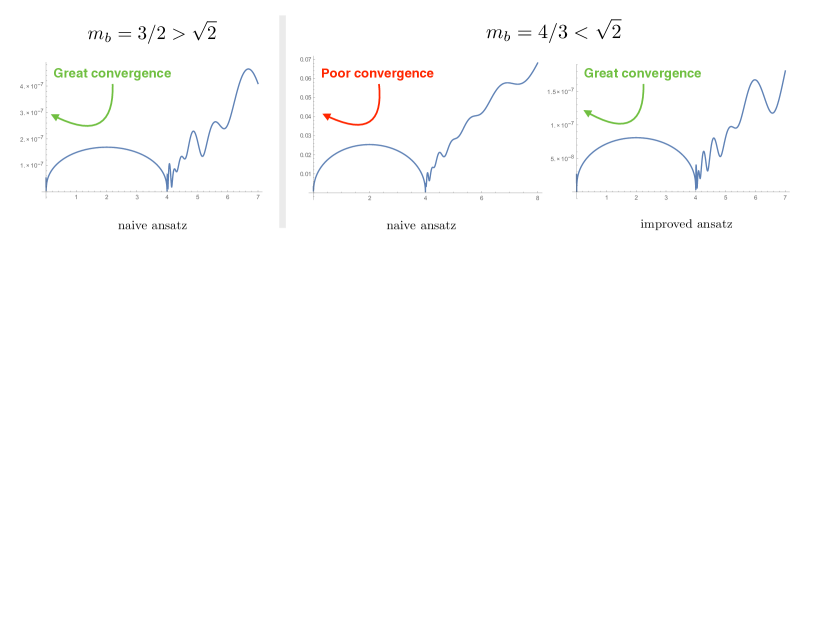
To be concrete we consider here the case where there is a single bound-state with mass $m_{b}$ whose coupling we maximize. The S-matrix with the largest coupling and such bound-state is given by [2]

$$S_{\text{max $g$}}=\text{sign}(m_{b}-\sqrt{2}m)\times\frac{\sqrt{s(s-4m^{2})}+\sqrt{m_{b}^{2}(4m^{2}-m_{b}^{2})}}{\sqrt{s(s-4m^{2})}-\sqrt{m_{b}^{2}(4m^{2}-m_{b}^{2})}}$$ (121)

At high energies the S-matrix approaches $+1$ for $m_{b}>\sqrt{2}m$ and $-1$ for $m_{b}<\sqrt{2}m$ and this leads to a very different behavior when translated to the amplitude $M$. In particular, for a light bound state $m_{b}<\sqrt{2}m$ we see that the amplitude $M$ in (119) must diverge at high energies so that the right hand side approaches $-2$. This is hard for an ansatz a la (3) to achieve, that is it would require that the sum in

$$M_{\text{naive}}(s,t)=-\frac{\hat{g}^{2}}{s-m_{b}^{2}}-\frac{\hat{g}^{2}}{t-m_{b}^{2}}+\sum_{a,b=0}^{\Lambda}c_{ab}\,\rho_{s}^{a}\rho_{t}^{b}$$ (122)

to develop a divergence as $s=4m^{2}-t\to\infty$ which corresponds to $\rho_{s},\rho_{t}\to-1$. Such non-analytic behavior at the boundary of the unit disc can be achieved but a numerically sufficiently accurate approximation requires very large $\Lambda$.

In this case there is however a very obvious improvement which is to simply allow for a divergence at large energies which is after all allowed by unitarity and write down instead an ansatz of the form

$$M_{\text{improved}}(s,t)=-\frac{\hat{g}^{2}}{s-m_{b}^{2}}-\frac{\hat{g}^{2}}{t-m_{b}^{2}}+\sum_{a,b=0}^{\Lambda-2}c_{ab}\,\rho_{s}^{a}\rho_{t}^{b}+\frac{\beta}{\sqrt{\rho_{s}+1}\sqrt{\rho_{t}+1}}+\frac{\tilde{\beta}}{(\rho_{s}+1)(\rho_{t}+1)}$$ (123)

This immediately allows for a more general high energy behavior and thus an extreme improvement in convergence as illustrated in figure 15.

The moral of this story seems to be that we better allow for flexible ansatze which can easily capture various analytic properties of scattering amplitudes if we want to achieve optimal convergence. In this simple two dimensional example, allowing for an ansatz with a more flexible high energy behavior led to a drastic improvement in the numerics.

References

- [1] M. F. Paulos, J. Penedones, J. Toledo, B. C. van Rees, and P. Vieira, “The S-matrix Bootstrap I: QFT in AdS,” arXiv:1607.06109 [hep-th].
- [2] M. F. Paulos, J. Penedones, J. Toledo, B. C. van Rees, and P. Vieira, “The S-matrix Bootstrap II: Two Dimensional Amplitudes,” arXiv:1607.06110 [hep-th].
- [3] M. Creutz, “Rigorous bounds on coupling constants in two-dimensional field theories,” Physical Review D 6 no. 10, (1972) 2763.
- [4] M. Hogervorst and S. Rychkov, “Radial Coordinates for Conformal Blocks,” Phys.Rev. D87 (2013) 106004, arXiv:1303.1111 [hep-th].
- [5] X. O. Camanho, J. D. Edelstein, J. Maldacena, and A. Zhiboedov, “Causality Constraints on Corrections to the Graviton Three-Point Coupling,” JHEP 02 (2016) 020, arXiv:1407.5597 [hep-th].
- [6] S. Weinberg, The Quantum theory of fields. Vol. 1: Foundations. Cambridge University Press, 2005.
- [7] J. Bros, H. Epstein, and V. Glaser, “A proof of the crossing property for two-particle amplitudes in general quantum field theory,” Commun. Math. Phys. 1 no. 3, (1965) 240–264.
- [8] A. Martin, “Rigorous results from theory and unitarity,” Tech. Rep. CERN-TH-1181, CERN, Geneva, 1970. https://cds.cern.ch/record/944356.
- [9] J. D. Bjorken and S. D. Drell, “Relativistic quantum fields,”.
- [10] A. Martin, Scattering theory: unitarity, analyticity and crossing. Springer, 1969.
- [11] F. J. Yndurain, “Rigorous constraints, bounds, and relations for scattering amplitudes,” Rev. Mod. Phys. 44 (1972) 645–667.
- [12] S. Caron-Huot, Z. Komargodski, A. Sever, and A. Zhiboedov, “Strings from Massive Higher Spins: The Asymptotic Uniqueness of the Veneziano Amplitude,” arXiv:1607.04253 [hep-th].
- [13] A. Sever and A. Zhiboedov, “On Fine Structure of Strings: The Universal Correction to the Veneziano Amplitude,” arXiv:1707.05270 [hep-th].
- [14] F. Forstnerivc, Stein manifolds and holomorphic mappings: The homotopy principle in complex analysis, vol. 56. Springer Science & Business Media, 2011.
- [15] V. F. Müller, “An upper bound on the coupling constant of scalar mesons,” Il Nuovo Cimento A (1971-1996) 42 no. 1, (Mar, 1966) 185–189. http://dx.doi.org/10.1007/BF02856203.
- [16] G. Auberson, L. Epele, and F. R. A. Simao, “Almost Optimality of an Axiomatic Bound for pi0 pi0 Scattering,” Nucl. Phys. B133 (1978) 266–274.
- [17] C. Lopez and G. Mennessier, “Bounds on the pi0 pi0 Amplitude,” Nucl. Phys. B118 (1977) 426–444.
- [18] G. Auberson and G. Mennessier, “On the optimality of axiomatic constraints for pi0 pi0 scattering: The case of the lower bounds,” Nucl. Phys. B162 (1980) 440–448.
- [19] S. R. Coleman, “More About the Massive Schwinger Model,” Annals Phys. 101 (1976) 239.
- [20] I. Caprini and P. Dita, “A new method for deriving rigorous results on pi pi scattering,” J. Phys. A13 (1980) 1265–1286.
- [21] C. Lopez and G. Mennessier, “A New Absolute Bound on the pi0 pi0 S-Wave Scattering Length,” Phys. Lett. 58B (1975) 437–441.
- [22] L. Lukaszuk and A. Martin, “Absolute upper bounds for pi pi scattering,” Nuovo Cim. A52 (1967) 122–145.
- [23] B. Bonnier and R. V. Mau, “Connection between the Wigner Inequalities and Analyticity and Unitarity,” Phys. Rev. 165 (1968) 1923–1926.
- [24] B. Bonnier, “Derivation and Implications of Rigorous Absolute Bounds for pi pi Partial Waves Up to 1-GeV,” Nucl. Phys. B95 (1975) 98–108.
- [25] P. Dorey, “Exact S matrices,” in Conformal field theories and integrable models. Proceedings, Eotvos Graduate Course, Budapest, Hungary, August 13-18, 1996, pp. 85–125. 1996. arXiv:hep-th/9810026 [hep-th].
- [26] S. O. Aks, “Proof that scattering implies production in quantum field theory,” Journal of Mathematical Physics 6 no. 4, (1965) 516–532.
- [27] A. Dragt, “Amount of four-particle production required in s-matrix theory,” Physical Review 156 no. 5, (1967) 1588.
- [28] S. Mandelstam, “Analytic properties of transition amplitudes in perturbation theory,” Phys. Rev. 115 (1959) 1741–1751.
- [29] M. Ruderman and S. Gasiorowicz, “Limits on coupling constants in field theories with finite sources,” Il Nuovo Cimento (1955-1965) 8 no. 6, (1958) 861–877.
- [30] V. Gribov, Y. B. Zel’dovich, and A. Perelomov, “On the maximal charge for a given mass of the bound state,” Zhur. Eksptl’. i Teoret. Fiz. 40 (1961) .
- [31] D. Simmons-Duffin, “A Semidefinite Program Solver for the Conformal Bootstrap,” JHEP 06 (2015) 174, arXiv:1502.02033 [hep-th].