DIII Topological Superconductivity with Emergent Time-Reversal Symmetry
Abstract
We find a new class of topological superconductors which possess an emergent time-reversal symmetry that is present only after projecting to an effective low-dimensional model. We show that a topological phase in symmetry class DIII can be realized in a noninteracting system coupled to an -wave superconductor only if the physical time-reversal symmetry of the system is broken, and we provide three general criteria that must be satisfied in order to have such a phase. We also provide an explicit model which realizes the class DIII topological superconductor in 1D. We show that, just as in time-reversal invariant topological superconductors, the topological phase is characterized by a Kramers pair of Majorana fermions that are protected by the emergent time-reversal symmetry.
pacs:
74.45.+c,71.10.Pm,73.21.Hb,74.78.NaIntroduction.
Topological superconductors have been intensively pursued in recent years Alicea (2012); Leijnse and Flensberg (2012); Beenakker (2013) because the Majorana fermions which are localized to their boundaries have potential applications in the development of a topological quantum computer Kitaev (2001); Nayak et al. (2008). The most promising proposals to date for engineering topological superconductivity involve coupling a conventional superconductor either to a nanowire with Rashba spin-orbit interaction that is subjected to an external magnetic field Lutchyn et al. (2010); Oreg et al. (2010); Mourik et al. (2012); Deng et al. (2012); Das et al. (2012); Rokhinson et al. (2012); Churchill et al. (2013); Finck et al. (2013); Chang et al. (2015); Albrecht et al. (2016); Deng et al. (2016); Zhang et al. (2017) or to a ferromagnetic atomic chain Nadj-Perge et al. (2013); Pientka et al. (2013); Klinovaja et al. (2013); Vazifeh and Franz (2013); Braunecker and Simon (2013); Nadj-Perge et al. (2014); Peng et al. (2015); Pawlak et al. (2016).
Additionally, there have been several proposals to engineer topological superconductors in symmetry class DIII. Such systems possess both particle-hole symmetry and time-reversal symmetry Schnyder et al. (2008), with the presence of time-reversal symmetry ensuring that the Majorana fermions existing at the boundaries of class DIII topological superconductors come in Kramers pairs. In one dimension (1D), where superconductivity is required to be induced by the proximity effect, it has been shown that a nontrivial topological phase in class DIII can be realized by proximity coupling a noninteracting multichannel Rashba nanowire to an unconventional superconductor Wong and Law (2012); Nakosai et al. (2013); Zhang et al. (2013); Dumitrescu et al. (2014) or to two conventional superconductors forming a Josephson junction with a phase difference of Keselman et al. (2013). Alternatively, an effective -phase difference can be induced in a multichannel Rashba nanowire with repuslive electron-electron interactions Haim et al. (2014) or in a system of two topological insulators coupled to a conventional superconductor via a magnetic insulator Schrade et al. (2015). It has also been proposed to realize class DIII topological superconductivity in a system of two Rashba nanowires Klinovaja and Loss (2014); Gaidamauskas et al. (2014); Schrade et al. (2017) or two topological insulators Klinovaja et al. (2014) coupled to a single conventional superconductor, but repulsive interactions are also necessary to reach the topological phase in these setups, which require a strength of induced crossed Andreev (interwire) pairing exceeding that of the direct (intrawire) pairing Reeg et al. (2017); Recher and Loss (2002); Bena et al. (2002). While it would be beneficial to engineer a DIII topological superconductor in a noninteracting 1D system coupled to a single conventional superconductor, as such a setup could avoid relying on unconventional superconductivity or interactions that are difficult to control experimentally, it was recently shown that this is not possible in a fully time-reversal invariant system Haim et al. (2016).
In this paper, we show that such a 1D topological superconductor in class DIII can be realized when time-reversal symmetry is explicitly broken. While the full Hamiltonian (describing the 1D system, the superconductor, and the tunnel coupling) possesses only particle-hole symmetry and is thus in symmetry class D, it is possible to place the system in symmetry class DIII after integrating out the superconductor Sau et al. (2010); Potter and Lee (2011); Kopnin and Melnikov (2011); Zyuzin et al. (2013); van Heck et al. (2016); Reeg and Maslov (2017); Reeg et al. (2017, ) and projecting to an effective 1D model not (a). We establish three necessary criteria to realize a DIII topological phase. First, the 1D system must obey an “emergent” time-reversal symmetry. That is, given the Hamiltonian density of the 1D system, there must exist a unitary matrix such that and . [While a specific example could be the physical time-reversal symmetry , where is a Pauli matrix acting in spin space, we do not restrict ourselves to this case.] Second, the self-energy induced on the 1D system by the superconductor must preserve the emergent time-reversal symmetry. Third, the anomalous (pairing) component of the self-energy must have both positive and negative eigenvalues.
After a general discussion, we provide a simple model which realizes the DIII topological phase in 1D. We consider a system of two Rashba nanowires with opposite Zeeman splittings coupled to an -wave superconductor. We show that such a system undergoes a topological phase transition under certain conditions. By explicitly solving for the wave functions of the Majorana bound states, we show that the topological phase is characterized by the presence of a Kramers pair of Majorana fermions that is protected by the emergent time-reversal symmetry.
Minimum requirements for DIII topological phase.
We consider a general 1D (noninteracting) system coupled to a conventional superconductor. We assume that the system is translationally invariant along the direction of the 1D system, allowing us to define a conserved momentum . The Hamiltonian of the 1D system is given by
| (1) |
where is a spinor annihilation operator acting on all internal degrees of freedom of the 1D system (spin, subband, etc.) and is a Hermitian matrix. We assume that there exists a unitary matrix which acts as an effective time-reversal symmetry on the Hamiltonian, such that and . Introducing the Nambu spinor , the Hamiltonian Eq. (1) can be expressed as
| (2) |
where and is a Pauli matrix acting in Nambu space.
The 1D system is coupled to a conventional superconductor which is described by a BCS Hamiltonian,
| (3) |
where denotes directions transverse to the 1D system and is a spinor creation operator in Nambu spin space. The Hamiltonian density in this basis is given by , where , , and are the effective mass, chemical potential, and pairing potential of the superconductor, respectively. The superconductor is time-reversal invariant, , where is the physical time-reversal operator, with the Pauli matrix acting in spin space.
We allow for a linear coupling between the 1D system and the superconductor of the form
| (4) |
The tunneling matrix in Nambu space, , can be expressed generally as
| (5) |
where , , and is a tunneling matrix acting on all additional degrees of freedom in the system not (b). Combining Eqs. (2)-(4), the full Hamiltonian can be expressed as
| (6) |
where we suppress explicit reference to for brevity. Note that the time-reversal symmetry of the full Hamiltonian is broken by having ; i.e., , where is the Hamiltonian density of Eq. (6) and . For this reason, it was assumed that in Ref. Haim et al. (2016).
We now project our system to an effective 1D model by integrating out the superconductor Sau et al. (2010); Potter and Lee (2011); Kopnin and Melnikov (2011); Zyuzin et al. (2013); van Heck et al. (2016); Reeg and Maslov (2017); Reeg et al. (2017, ). The superconductor induces a self-energy on the 1D system given by
| (7) |
where is the Matsubara Green’s function of the bare superconductor, defined such that . In the limit of weak tunneling, where the relevant pairing energies in the 1D system are , it is sufficient to evaluate the self-energy at . In this case, the system is described by an effective 1D Hamiltonian given by . Since it was already assumed that obeys an effective time-reversal symmetry, the Hamiltonian is in class DIII if the self-energy of Eq. (7) preserves this symmetry,
| (8) |
Hence, acts as an emergent time-reversal symmetry which exists only in the low-dimensional subspace. Assuming that the self-energy satisfies Eq. (8), we can decompose it into normal and anomalous parts as
| (9) |
where and sup . In arriving at Eq. (9), we have utilized the fact that the superconducting Green’s function can be similarly decomposed as , where and are scalars.
The anomalous self-energy, which represents the induced pairing in the 1D system, can be expressed in a form
| (10) |
where . It was shown in Ref. Haim et al. (2016) that the class DIII topological invariant can only take a nontrivial value if has both positive and negative eigenvalues. It was also shown that is always positive semidefinite; hence, if the tunneling Hamiltonian is time-reversal invariant with , it is not possible to realize a topological phase. By extension, it is straightforward to show that must also be positive semidefinite. Consequently, the topological invariant must also take a trivial value if (in which case is negative semidefinite). However, if both terms in Eq. (10) are nonzero, is not restricted to be either positive semidefinite or negative semidefinite, and it is possible to have a topologically nontrivial phase.
We have thus established three minimal criteria to realize a class DIII topological phase in a noninteracting 1D system: the bare 1D system must obey an effective time-reversal symmetry, the self-energy induced by the superconductor must preserve this symmetry, and the anomalous self-energy must have both positive and negative eigenvalues. The final requirement can be satisfied only if the full tunneling Hamiltonian [Eq. (6)] is not time-reversal invariant. We will now provide a model which satisfies all three criteria, showing indeed that the class DIII topological phase can be realized.
Model.
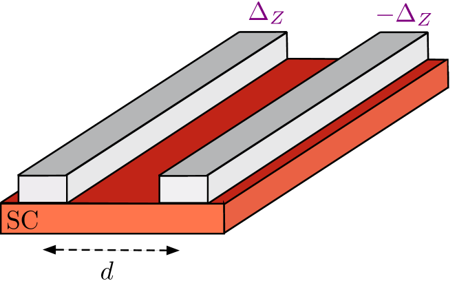
We consider the geometry shown in Fig. 1. Two Rashba nanowires, separated by a distance (let us take one wire to be located at and the other at ), are coupled to an infinite 2D -wave superconducting plane. We take the two nanowires to have opposite Zeeman splitting, which can be achieved by applying an antiparallel external magnetic field to each wire or by applying a uniform external magnetic field to two wires with opposite -factors.
The two nanowires are described by the Hamiltonian density
| (11) |
where ( is the effective mass and the chemical potential of the nanowires), is the Rashba spin-orbit interaction constant (we choose our spin quantization axis along the direction of the effective Rashba field), and is the Zeeman splitting in an external magnetic field of strength ( is the nanowire -factor and is the Bohr magneton). The Pauli matrix acts in left/right wire space. Crucially, we impose that the two nanowires are identical, with only a change in the sign of the Zeeman splitting. Although the Zeeman term in Eq. (11) explicitly breaks time-reversal, the Hamiltonian density obeys an effective time-reversal symmetry , where and .
The self-energy induced on the two nanowires by the superconductor is given in Eq. (7). Assuming that , we evaluate the Green’s function of the bulk 2D superconductor for momenta ( is the Fermi momentum of the superconductor) to give
| (12) | ||||
where is the coherence length and the Fermi velocity of the superconductor (we have also expanded in the limit ). We assume local spin- and momentum-independent tunneling of the form , where is a (scalar) tunneling amplitude which has the same strength in both nanowires. This gives and . Evaluating the self-energy Eq. (7), we find
| (13) |
where we define a single-particle interwire tunnel coupling , an induced direct (intrawire) pairing potential , and an induced crossed Andreev (interwire) pairing potential Reeg et al. (2017). Here, is a tunneling energy scale. Note that the pairing potentials always satisfy .
Taking into account the self-energy, the effective Hamiltonian describing the double nanowire system is given by
| (14) |
Because the self-energy preserves the effective time-reversal symmetry, , we also have . Additionally, the effective Hamiltonian possesses a particle-hole symmetry , where is a unitary matrix satisfying . Finally, the effective Hamiltonian possesses a chiral symmetry , where . These three properties of the Hamiltonian place it in the DIII symmetry class. Additionally, the anomalous self-energy has both positive and negative eigenvalues, . Because all of our previously established criteria are met in this setup, it is possible to have a topological phase.
To determine whether such a topological phase exists in this setup, we search for a gap-closing transition by enforcing . We find
| (15) | ||||
which yields a gap-closing at the critical Zeeman splitting . Therefore, in order to have a physical transition, the chemical potential of the nanowires must be tuned to . For simplicity, let us assume that the system is tuned in such a way that the interwire tunnel coupling vanishes, [which can be done by tuning ]. In this case, the critical Zeeman splitting at which the gap closes is given by
| (16) |
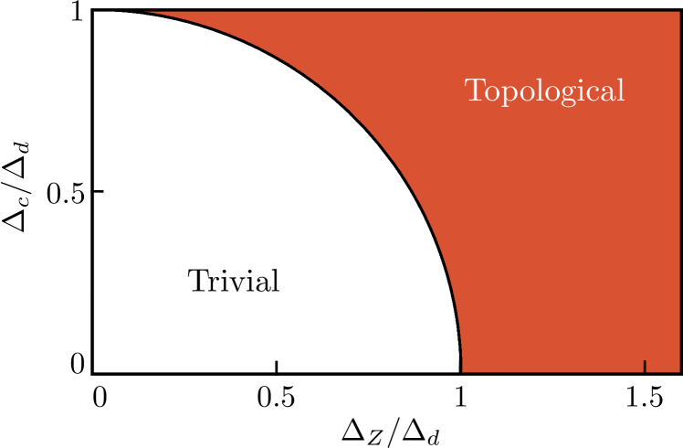
The phase diagram of our model is displayed in Fig. 2. We find two distinct phases whose topological characterization can be inferred along the line , corresponding to the case when the two wires are decoupled (). For , both wires are in a topologically trivial phase. For , both wires are in a topologically nontrivial phase, with each wire hosting its own distinct pair of Majorana bound states. Because the number of Majorana bound states is a topological invariant that cannot be changed without closing the gap, we conclude that corresponds to a topologically trivial phase while corresponds to a topologically nontrivial phase with two pairs of Majorana bound states.
To further establish the presence of a topologically nontrivial phase, we explicitly solve for the wave functions of the Majorana bound states. We now take our nanowires to be semi-infinite (), and we assume that the effective Hamiltonian of Eq. (14) remains valid for the semi-infinite case after replacing not (c). States in the nanowires obey a Bogoliubov-de Gennes equation given by . By constructing a general zero-energy solution and imposing a vanishing boundary condition , we find two Majorana bound state solutions in the topological phase () and no solutions in the trivial phase (). The full analytical expressions for the wave functions are given in the limit of strong spin-orbit interaction () in the Supplemental Material sup . We find that the two Majorana wave functions in the topological phase are orthogonal,
| (17) |
and related by the effective time-reversal symmetry,
| (18) | ||||
Hence, the two Majorana bound states in the system form a Kramers pair that is protected by the emergent time-reversal symmetry.
Conclusions.
We have shown that a topological superconductor in symmetry class DIII can be realized in a noninteracting 1D system proximity coupled to a conventional superconductor. Crucially, the full Hamiltonian (incorporating the 1D system, the parent superconductor, and the tunneling term) must not possess an effective time-reversal symmetry, with such a symmetry emerging only after projection to an effective 1D model. We provide an explicit example realizing such a class DIII topological superconductor, showing that the topological phase is characterized by a Kramers pair of Majorana bound states which is protected by the effective time-reversal symmetry of the system. We believe that our general criteria can be applied to realize class DIII topological superconductivity in a multitude of additional systems coupled to a bulk -wave superconductor, for example in nanowires with helical magnetization of opposite helicity, antiferromagnetically coupled spin chains, magnetic topological insulators with opposite magnetization, or ferromagnetic atomic chains with opposite magnetization.
Acknowledgments.
This work was supported by the Swiss National Science Foundation and the NCCR QSIT.
Note.
Upon completion of this manuscript, we became aware of a very recent preprint, Ref. Huang and Chiu , which discusses the realization of a class DIII topological phase in 2D antiferromagnetic quantum spin Hall insulators.
References
- Alicea (2012) J. Alicea, Rep. Prog. Phys. 75, 076501 (2012).
- Leijnse and Flensberg (2012) M. Leijnse and K. Flensberg, Semicond. Sci. Technol. 27, 124003 (2012).
- Beenakker (2013) C. W. J. Beenakker, Annu. Rev. Condens. Matter Phys. 4, 113 (2013).
- Kitaev (2001) A. Y. Kitaev, Physics-Uspekhi 44, 131 (2001).
- Nayak et al. (2008) C. Nayak, S. H. Simon, A. Stern, M. Freedman, and S. Das Sarma, Rev. Mod. Phys. 80, 1083 (2008).
- Lutchyn et al. (2010) R. M. Lutchyn, J. D. Sau, and S. Das Sarma, Phys. Rev. Lett. 105, 077001 (2010).
- Oreg et al. (2010) Y. Oreg, G. Refael, and F. von Oppen, Phys. Rev. Lett. 105, 177002 (2010).
- Mourik et al. (2012) V. Mourik, K. Zuo, S. M. Frolov, S. R. Plissard, E. P. A. M. Bakkers, and L. P. Kouwenhoven, Science 336, 1003 (2012).
- Deng et al. (2012) M. T. Deng, C. L. Yu, G. Y. Huang, M. Larsson, P. Caroff, and H. Q. Xu, Nano Letters 12, 6414 (2012).
- Das et al. (2012) A. Das, Y. Ronen, Y. Most, Y. Oreg, M. Heiblum, and H. Shtrikman, Nat. Phys. 8, 887 (2012).
- Rokhinson et al. (2012) L. P. Rokhinson, X. Liu, and J. K. Furdyna, Nat. Phys. 8, 795 (2012).
- Churchill et al. (2013) H. O. H. Churchill, V. Fatemi, K. Grove-Rasmussen, M. T. Deng, P. Caroff, H. Q. Xu, and C. M. Marcus, Phys. Rev. B 87, 241401 (2013).
- Finck et al. (2013) A. D. K. Finck, D. J. Van Harlingen, P. K. Mohseni, K. Jung, and X. Li, Phys. Rev. Lett. 110, 126406 (2013).
- Chang et al. (2015) W. Chang, S. M. Albrecht, T. S. Jespersen, F. Kuemmeth, P. Krogstrup, J. Nygård, and C. M. Marcus, Nat. Nano. 10, 232 (2015).
- Albrecht et al. (2016) S. M. Albrecht, A. P. Higginbotham, M. Madsen, F. Kuemmeth, T. S. Jespersen, J. Nygård, P. Krogstrup, and C. M. Marcus, Nature 531, 206 (2016).
- Deng et al. (2016) M. T. Deng, S. Vaitiekenas, E. B. Hansen, J. Danon, M. Leijnse, K. Flensberg, J. Nygård, P. Krogstrup, and C. M. Marcus, Science 354, 1557 (2016).
- Zhang et al. (2017) H. Zhang, Ö. Gül, S. Conesa-Boj, M. Nowak, M. Wimmer, K. Zuo, V. Mourik, F. K. de Vries, J. van Veen, M. W. A. de Moor, J. D. S. Bommer, D. J. van Woerkom, D. Car, S. R. Plissard, E. P. A. M. Bakkers, M. Quintero-Pérez, M. C. Cassidy, S. Koelling, S. Goswami, K. Watanabe, T. Taniguchi, and L. P. Kouwenhoven, Nat. Commun. 8, 16025 (2017).
- Nadj-Perge et al. (2013) S. Nadj-Perge, I. K. Drozdov, B. A. Bernevig, and A. Yazdani, Phys. Rev. B 88, 020407 (2013).
- Pientka et al. (2013) F. Pientka, L. I. Glazman, and F. von Oppen, Phys. Rev. B 88, 155420 (2013).
- Klinovaja et al. (2013) J. Klinovaja, P. Stano, A. Yazdani, and D. Loss, Phys. Rev. Lett. 111, 186805 (2013).
- Vazifeh and Franz (2013) M. M. Vazifeh and M. Franz, Phys. Rev. Lett. 111, 206802 (2013).
- Braunecker and Simon (2013) B. Braunecker and P. Simon, Phys. Rev. Lett. 111, 147202 (2013).
- Nadj-Perge et al. (2014) S. Nadj-Perge, I. K. Drozdov, J. Li, H. Chen, S. Jeon, J. Seo, A. H. MacDonald, B. A. Bernevig, and A. Yazdani, Science 346, 602 (2014).
- Peng et al. (2015) Y. Peng, F. Pientka, L. I. Glazman, and F. von Oppen, Phys. Rev. Lett. 114, 106801 (2015).
- Pawlak et al. (2016) R. Pawlak, M. Kisiel, J. Klinovaja, T. Meier, S. Kawai, T. Glatzel, D. Loss, and E. Meyer, Npj Quantum Information 2, 16035 (2016).
- Schnyder et al. (2008) A. P. Schnyder, S. Ryu, A. Furusaki, and A. W. W. Ludwig, Phys. Rev. B 78, 195125 (2008).
- Wong and Law (2012) C. L. M. Wong and K. T. Law, Phys. Rev. B 86, 184516 (2012).
- Nakosai et al. (2013) S. Nakosai, J. C. Budich, Y. Tanaka, B. Trauzettel, and N. Nagaosa, Phys. Rev. Lett. 110, 117002 (2013).
- Zhang et al. (2013) F. Zhang, C. L. Kane, and E. J. Mele, Phys. Rev. Lett. 111, 056402 (2013).
- Dumitrescu et al. (2014) E. Dumitrescu, J. D. Sau, and S. Tewari, Phys. Rev. B 90, 245438 (2014).
- Keselman et al. (2013) A. Keselman, L. Fu, A. Stern, and E. Berg, Phys. Rev. Lett. 111, 116402 (2013).
- Haim et al. (2014) A. Haim, A. Keselman, E. Berg, and Y. Oreg, Phys. Rev. B 89, 220504 (2014).
- Schrade et al. (2015) C. Schrade, A. A. Zyuzin, J. Klinovaja, and D. Loss, Phys. Rev. Lett. 115, 237001 (2015).
- Klinovaja and Loss (2014) J. Klinovaja and D. Loss, Phys. Rev. B 90, 045118 (2014).
- Gaidamauskas et al. (2014) E. Gaidamauskas, J. Paaske, and K. Flensberg, Phys. Rev. Lett. 112, 126402 (2014).
- Schrade et al. (2017) C. Schrade, M. Thakurathi, C. Reeg, S. Hoffman, J. Klinovaja, and D. Loss, Phys. Rev. B 96, 035306 (2017).
- Klinovaja et al. (2014) J. Klinovaja, A. Yacoby, and D. Loss, Phys. Rev. B 90, 155447 (2014).
- Reeg et al. (2017) C. Reeg, J. Klinovaja, and D. Loss, Phys. Rev. B 96, 081301 (2017).
- Recher and Loss (2002) P. Recher and D. Loss, Phys. Rev. B 65, 165327 (2002).
- Bena et al. (2002) C. Bena, S. Vishveshwara, L. Balents, and M. P. A. Fisher, Phys. Rev. Lett. 89, 037901 (2002).
- Haim et al. (2016) A. Haim, E. Berg, K. Flensberg, and Y. Oreg, Phys. Rev. B 94, 161110 (2016).
- Sau et al. (2010) J. D. Sau, R. M. Lutchyn, S. Tewari, and S. Das Sarma, Phys. Rev. B 82, 094522 (2010).
- Potter and Lee (2011) A. C. Potter and P. A. Lee, Phys. Rev. B 83, 184520 (2011).
- Kopnin and Melnikov (2011) N. B. Kopnin and A. S. Melnikov, Phys. Rev. B 84, 064524 (2011).
- Zyuzin et al. (2013) A. A. Zyuzin, D. Rainis, J. Klinovaja, and D. Loss, Phys. Rev. Lett. 111, 056802 (2013).
- van Heck et al. (2016) B. van Heck, R. M. Lutchyn, and L. I. Glazman, Phys. Rev. B 93, 235431 (2016).
- Reeg and Maslov (2017) C. Reeg and D. L. Maslov, Phys. Rev. B 95, 205439 (2017).
- (48) C. Reeg, D. Loss, and J. Klinovaja, arXiv:1707.08417 .
- not (a) This is analogous to the conventional Majorana proposal of a single Rashba nanowire coupled to an -wave superconductor and subjected to an external magnetic field. In this setup, the field breaks time-reversal symmetry and places the full Hamiltonian in class D. However, after projecting to 1D, it is possible to define an effective time-reversal symmetry (which squares to ), thus placing the 1D system in class BDI Tewari and Sau (2012).
- not (b) Note that we do not consider the possibility that is a two-body operator as in Ref. Schrade et al. (2015), as this corresponds to an interacting model.
- (51) See Supplemental Material for a derivation of Eq. (9) and a detailed solution for the Majorana wave functions of our model.
- not (c) Because the proximity effect was treated in the bulk of the nanowires, there could be additional boundary effects that are not properly accounted for in the effective Hamiltonian. However, the presence or absence of topological Majorana modes is insensitive to such boundary effects.
- (53) Y. Huang and C.-K. Chiu, arXiv:1708.05724 .
- Tewari and Sau (2012) S. Tewari and J. D. Sau, Phys. Rev. Lett. 109, 150408 (2012).
I Supplemental Material
A Form of Self-Energy
In this section, we prove that the self-energy can be decomposed into normal and anomalous components as in Eq. (9) of the main text. The self-energy of the effective 1D model is given by
| (S1) |
Substituting the tunneling term , and noting that the superconducting Green’s function (at ) can be decomposed into normal and anomalous parts as , where and are scalars, we find a self-energy given by (we suppress explicit reference to the transverse coordinates and for brevity)
| (S2) |
We now require the self-energy to preserve the effective time-reversal symmetry of the 1D system by enforcing . Because the four terms of Eq. (S2) are linearly independent, each term must separately obey this condition.
Let us first consider the term proportional to ; expanding out this term using the definitions and gives
| (S3) |
Applying the time-reversal operator to Eq. (S3) and using the fact that , we see that in order to preserve the time-reversal symmetry of the 1D system, the self-energy must satisfy
| (S4) |
or, equivalently,
| (S5) |
Hence, the term proportional to in Eq. (S2) must vanish.
B Majorana Wave Functions
In this section, we explicitly solve for the Majorana wave functions in a semi-infinite geometry. States in the nanowire obey a Bogoliubov-de Gennes equation given by
| (S10) |
where is a spinor wave function and is given by
| (S11) |
Because the wires are semi-infinite, Majorana solutions are necessarily at zero energy. Setting , we rewrite Eq. (S10) in the form
| (S12) |
where and
| (S13) |
Any zero-energy solution to Eq. (S10) can be written in the form
| (S14) |
where are the eigenvalues of and are the corresponding eigenvectors.
Eigenvalues of must satisfy (for brevity, we temporarily set )
| (S15) | ||||
While this equation cannot be solved analytically in general, we can solve it in the limit of strong spin-orbit interaction, . First, we expand in the vicinity of the exterior branches of the spectrum by setting and expanding for . We find
| (S16) |
Therefore, at both the positive and negative exterior branches, we find four allowed momenta with . Next, we expand in the vicinity of the interior branches of the spectrum by setting and again expanding for ; we find
| (S17) |
For the interior branches, we find four doubly degenerate momenta corresponding to .
For bound states, only momenta with positive imaginary part are allowed. Restoring the factors of , the allowed momenta in the topological phase () are given by
| (S18) | ||||
Substituting Eqs. (S18) and (S14) into Eq. (S10) and similarly expanding in the limit of strong spin-orbit interaction, we find the corresponding eigenvectors
| (S19) | ||||
where we define .
The coefficients are determined by imposing the boundary condition . We find two solutions given by
| (S20) | ||||
where are normalization constants. The wave functions are normalized according to
| (S21) |
Evaluating the integral, we find normalization constants
| (S22) | ||||
Substituting Eq. (S22) into Eq. (S20), we see that the two Majorana wave functions are orthogonal,
| (S23) |
and related by the emergent time-reversal symmetry (),
| (S24) | ||||
Hence, the two Majorana bound states form a Kramers pair that is protected by the emergent time-reversal symmetry.