Earthquakes economic costs through rank-size laws

Abstract

This paper is devoted to assess the presence of some regularities in the magnitudes of the earthquakes in Italy between January $24^{th}$, 2016 and January $24^{th}$, 2017, and to propose an earthquakes cost indicator. The considered data includes the catastrophic events in Amatrice and in Marche region. To our purpose, we implement two typologies of rank-size analysis: the classical Zipf-Mandelbrot law and the so-called universal law proposed by Cerqueti and Ausloos (2016). The proposed generic measure of the economic impact of earthquakes moves from the assumption of the existence of a cause-effect relation between earthquakes magnitudes and economic costs. At this aim, we hypothesize that such a relation can be formalized in a functional way to show how infrastructure resistance affects the cost. Results allow us to clarify the impact of an earthquake on the social context and might serve for strengthen the struggle against the dramatic outcomes of such natural phenomena.

Keywords: Earthquake, magnitude, economic cost, Zipf-Mandelbrot law, rank-size analysis, Italy.

1 Introduction

Seismologists have carefully clustered the world in different non-overlapping zones on the basis of the probability that the zone experiences an earthquake. Such natural phenomena might cause very dramatic damages to the human activities and kill several people. Thus, policymakers should adopt anti-seismic building strategies, mainly in zones with a high seismic risk. Unfortunately, some countries come from a political history of myopic decisions in this respect, and Italy is an illustrative example of them.
This paper aims at exploring the Italian earthquakes occurred in 2016 and early 2017, with a specific reference to the big ones in Amatrice (August, $24^{th}$) and Visso (October, $26^{th}$ – two times – and $30^{th}$) along with the large amount of minor earthquakes before and after them. The considered period is 365 days, from January 24, 2016 to January 24, 2017, along which we observe 978 seismic events within a Richter magnitude range: [3.1 - 6.5]. We decide to exclude observations with magnitudes smaller than 3.1 for many reasons. First of all, this paper deals with formulations of damages’ cost indicators of the earthquakes and according to the United States Geological Survey, a seismic event with magnitude less than 3.1 has very low probability to cause observable damages. Secondly, the restriction to magnitudes not smaller than 3.1 allows to face the incomplete catalog problem. Indeed, we are analyzing a peculiar time period from a seismic point of view. Such a period has given a lot of work to the Italian National Institute of Geophysics and Vulcanology (INGV) because of the high number of earthquakes concentrated in very short time and of the intensity of them. In fact, after the mainshock of Amatrice, SISMIKO, the coordinating body of the emergency seismic network at INGV, was activated to install a temporary seismic network integrated with the existing permanent network in the epicentral area, but the risk that many aftershocks were not registered or not revised remains high (see Moretti et al., 2016). On this point, some scholars are actively working on the estimation of the catalog completeness. For example, Marchetti et al. (2016) have estimated $M_{c}=2.7$ for the revised catalog of the seismic events occurred immediately after the Amatrice’s earthquake. In accord to Marchetti et al’s work, $M_{c}$ could rise to a maximum level of 3.1 (on this topic see also Chiaraluce et al., 2017).
Moreover, our dataset has no particular peaks apart from those showed in Figure 1 after August $24^{th}$. Then, from the 24/01/2016 to 23/08/2016, we can consider $M_{c}=2.5$, in accord to Romashkova and Peresan (2013) and Schorlemmer et al. (2010).
Thus, the considered restriction to magnitudes greater than 3.1 let prudentially the catalog incompleteness problem be quite negligible in the reference period without affecting the cost analysis of the earthquakes.
We propose here a rank-size approach for analyzing the earthquakes’ magnitudes sequence just described in order to assess the presence of data regularities.
The rank-size relationship has been explored for several sets of data and it is still at the center of the scientific debate. At its inception, power law and Pareto distribution with unitary coefficient, introduced in Zipf (1935, 1949) and denoted from there as Zipf law, has been suitably employed to provide a best fit of the rank-size connections in the field of linguistics.
After the first applications, several contributions supporting the validity of the Zipf law have appeared in the literature. In this respect, we just mention some recent important papers: Ioannides and Overman (2003), Gabaix and Ioannides (2004), Dimitrova and Ausloos (2015), Cerqueti and Ausloos (2015) in the context of economic geography; Montemurro (2001) and Piantadosi (2014) in linguistic; Axtell (2001), Fujiwara (2004), Bottazzi at al (2015) in the business size field; Li and Yan (2002) in biology; Levene, Borges and Loizou (2001) and Maillart et al (2008) in informatics; Manaris et al (2005) and Zanette (2006), in the context of music; Huang et al (2008) in the context of fraud detection; Blasius and Tönjes (2009) in the gaming field. For a wide review of rank-size analysis see Pinto et al (2012). However, some cases of rank-size relationships fail to be well-fitted by Zipf law (see e.g. Rosen and Resnick, 1980; Peng, 2010; Ioannides and Skouras, 2013; Matlaba et al., 2013). By one side, such examples support the acknowledged lack of a theoretical ground for this statistical regularity (see Fujita et al., 1999; Fujita and Thisse, 2000); by the other side, they represent a further hint for proceeding with the methodological research, and construct more general laws.
Indeed, under a pure methodological point of view, several extensions of the Zipf law have been introduced. The most prominent examples are the Zipf-Mandelbrot law (ZML, hereafter; see Mandelbrot, 1953, 1961; Fairthorne, 2005) and the Lavalette law (LL hereafter; see Lavalette, 1966), which have been proven to provide a spectacular fit of rank-size relations, even when Zipf law fails to do it (see e.g. Cerqueti and Ausloos, 2015).
In this paper, we implement two general rank-size procedures: the above-mentioned ZML and a universal law (UL from now on), which is an extension of the LL to a five parameters rule that has been recently introduced by Cerqueti and Ausloos (2016). All fits have been carried out through a Levenberg-Marquardt algorithm (Levenberg 1944, Marquardt 1963, Lourakis 2005) with a restriction on the parameters that have to be positive.
Furthermore, we have also discussed the economic costs of the earthquakes. At this aim, we propose a new generic cost indicator based on a suitable transformation of magnitudes into costs. As we will see, such an indicator moves from the best fit procedures implemented in the rank-size analysis phase, and it might be effectively used for finalizing policies for the management of seismic risks. We show how the cost indicator can be computed in the special case of the analyzed earthquakes.
Rank-size relations have been introduced for the explanation of seismological data and for the earthquakes magnitudes (see e.g. Jaume, 2000; Wu, 2000; Mega et al, 2003; Newman, 2005; Saichev and Sornette, 2006; Pinto et al, 2012; Aguilar-San Juan and Guzman-Vargas, 2013). However, this is the first paper which treats very recent Italian seismic events under this perspective. Moreover, to the best of our knowledge, there are no contributions in the literature on the construction of a cost indicator for earthquakes based on the rank-size laws.
In order to validate the obtained results, extra investigations on two different datasets have been performed. The first deals with a more global analysis on the basis of a suitable enlargement of the dtaset. At this aim, we notice that an important change of Italian seismic network is occurred in $16^{th}$ April, 2005, when the new network for seismic events collection has been activated. From that date the data elaboration system has sensibly increased and, in order to deal with the incompleteness catalog problem, the accepted average $M_{c}$ has been set to 2.5 (see Romashkova and Peresan 2013, and Schorlemmer et al. 2010). Therefore, we have performed the rank-size analysis on the data from the INGV catalog in the period ranging from 16/04/2005 to 31/03/2017, with the restriction to magnitudes not smaller than 2.5.
The second extra investigation is developed to face the effects of space variables. In this case, the considered dataset has been created by selecting the earthquakes with epicenters in the eight adjacent provinces involved in the seismic sequence started with the Amatrice’s earthquake: Macerata, Perugia, Rieti, Ascoli Piceno, L’Aquila, Teramo, Terni and Fermo (and respective coasts), from 24/01/2016 to 24/01/2017. In so doing, we are in line with geophysicists who claim that taking a small region and a short time period let the space effects be not relevant (see e.g. De Natale et al., 1988). It is interesting to note that, as we will see, the local analysis is not too different from the original one in terms of the cardinality of the dataset, in that the most part of the earthquakes in the reference period in Italy has occurred in such eight provinces.
The rest of the paper is organized as follows: Section 2 is devoted to the description of the data and of the methodologies used for performing the analysis. This section illustrates also the procedure adopted for the identification of the earthquakes costs and for the development of the cost indicator. Section 3 investigates the robustness of the reached results by presenting the study of the global and local datasets. Section 4 proposes the results of the analysis, along with a critical discussion of them. Last Section concludes and offers directions for future research.

2 Data and methodology

This section is devoted to the description of the data on the magnitudes of the earthquakes occurred in Italy in 2016 and early 2017. Furthermore, it contains the illustration of the methodological tools used for analysis.

2.1 Data

Our dataset is composed by the magnitudes of the earthquakes registered in Italy during the period: January $24^{th}$, 2016 - January $24^{th}$, 2017.
The definition of the magnitude of an earthquake and the employed dataset are taken from the website of the INGV (the Italian National Institute of Geophysics and Vulcanology see <http://cnt.rm.ingv.it/>). Such a definition is based on the different measurement methods used from seismograms, each of them being also tailored on a specific magnitude range and epicentral distance. For the details on the concept of magnitude, please refer to the website of the INGV (see <http://cnt.rm.ingv.it/en/help/>).
Specifically, the considered period starts at the first hour of January $24^{th}$,2016 and ends on the midnight of January $24^{th}$, 2017, hence including relevant earthquakes like those registered in Amatrice, on August $24^{th}$ (magnitude equals to 6) Umbria and Marche regions on October $26^{th}$ (two times) and $30^{th}$ of 2016 (magnitudes 5.4, 5.9 and 6.5 respectively), and the most recent on January $18^{th}$ 2017, in L’Aquila (three times, magnitude 5.5, 5.4 and 5.1). To have an idea of the seismic activity of the analyzed period, see Figure 1.

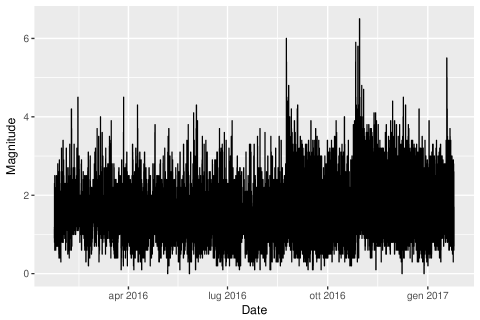
Figure 1: The time series of the earthquakes occurred from $24^{th}$ January 2016 to $24^{th}$ January 2017, according to the INGV data. The number of observations is 59190.

The number of the available data is of high relevance. Indeed, the number of registered seismic events over the considered period is 59190, which gives to the reader the dimension of how often earthquakes are registered in this period in Italy, in particular in the Center of Italy, since the majority of the earthquakes are located there. Data on depth of the epicenters and on their localization are also available, but they are not treated in this study. They are left for future researches.
We need to point out that there is a catalog incompleteness problem, in that the main events might hide several minor subsequent aftershocks. In order to deal with such catalog incompleteness problem, we restrict the analysis to the seismic events of magnitude not smaller than 3.1 (see Section 1 for a detailed discussion of this point). Therefore, the number of observations reduces to 978. Table 1 collects the main statistical indicators of the data and Figure 2 represent the probability density function of the considered time series. Notice that Figure 2 contains also the best fit of a power law function with the empirical distribution of the sizes of the earthquakes. This supports an empirical evidence, already pointed out by previous studies (see e.g. Kagan, 2010). Some comments on the statistical characteristics can be found in Section 4.

Statistical indicator	Value
Number of data	978
Maximum	6.50
Minimum	3.10
Mean ($\mu$)	3.42
Median ($m$)	3.30
RMS	3.45
Standard Deviation ($\sigma$)	0.39
Variance	0.15
Standard Error	0.01
Skewness	2.67
Kurtosis	14.36
$\mu/\sigma$	8.73
$3(\mu-m)/\sigma$	0.95

Table 1: Summary of the statistical characteristics for the magnitudes not smaller than 3.1 of the earthquakes in Italy during 365 days: from January $24^{th}$, 2016 to January $24^{th}$, 2017.

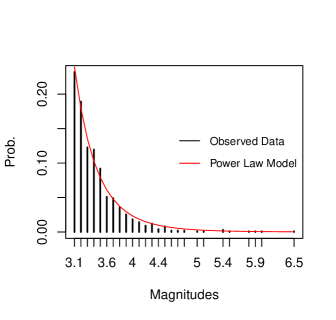
Figure 2: Probability density function of all the earthquakes registered from 24/01/2016 to 24/01/2017 with magnitudes not smaller than 3.1. The best fit of the empirical distribution with a power law of the type $y=ax^{b}$ is also shown. The calibrated parameters are $\hat{a}=7428.58$ and $\hat{b}=-9.14$, with an $R^{2}$ of 0.99.

2.2 Methodologies

The magnitude of an earthquake represents the size of the rank-size analysis.
Since the target of the analysis is to construct an aggregated costs indicator, magnitudes are not taken as they are. Indeed, the same earthquake can produce different levels of damages if it follows a long list of foreshocks or not: in the former case, the earthquake insists over an already solicited territory, while in the latter one it is the first shake and human activities have not previous solicitations. Therefore, each earthquake has been temporally contextualized – suppose, it has occurred at time $t$ – and we have transformed its magnitude $z$ into $\tilde{z}=\eta(n,z_{1},\dots,z_{n},\Delta t)\times z$, where $\eta(n,z_{1},\dots,z_{n},\Delta t)$ is a parameter dependent on the number $n$ of the foreshocks whose magnitudes are assumed to be $z_{1},\dots,z_{n}$ and occurred in the time interval $[t-\Delta t,t]$. The parameter $\eta(n,z_{1},\dots,z_{n},\Delta t)$ is marginally increasing with respect to $z_{1},\dots,z_{n}$ and $n$ and marginally decreasing with respect to $\Delta t$, and it is not smaller than 1. In fact, if the territory has experienced several foreshocks of large magnitude in a small time range before $t$, then the damages created by the earthquake are comparable with those of an isolated earthquake with magnitude $\tilde{z}>z$.
With a reasonable abuse of notation, we refer hereafter simply to magnitudes, having in mind $\tilde{z}$ instead of $z$.
The single earthquakes have been ranked in decreasing order, so that rank $r=1$ corresponds to the highest registered magnitude while $r=978$ is associated to the lowest value of the considered phenomenon, which is 3.1. Then, in general, low ranks are the ones associated to the strongest seismic events in terms of magnitudes, while high ranks point to the earthquakes with small magnitudes.
Here we implement two times the best fit procedure to assess whenever the size-magnitude $z$ might be view as a function of the rank $r$. The considered fit functions are the ZML and the UL. The former can be written as

$$\tilde{z}\sim f_{ZML}(r)=\alpha(r+\beta)^{-\gamma},$$ (1)

while the latter is

$$\tilde{z}\sim f_{UL}(r)=k\dfrac{\left(N+1-r+\psi\right)^{\xi}}{\left[N(r+\phi)\right]^{\lambda}},$$ (2)

where $\alpha$, $\beta$, $\gamma$ must be calibrated on the size data when (1) is used, while $k$, $\psi$, $\xi$, $\phi$, $\lambda$ are those to be calibrated if the fit procedure is as in (2). The parameter $N$ corresponds to the number of observations, and it is $N=978$ for this specific case.
To implement the rank-size analysis and derive the proposed aggregated cost indicator we need to provide an explicit shape of the parameter $\eta(n,z_{1},\dots,z_{n},\Delta t)$. In order to meet space constraints, we present here the analysis of the unbiased scenario of $\eta(n,z_{1},\dots,z_{n},\Delta t)=1$, for each $n,z_{1},\dots,z_{n},\Delta t$. In this case we are in absence of amplification effects. Since we aim at constructing an aggregated cost indicator, this situation has an intuitive reasoning: indeed, it is the case with the lowest level of damages – all the earthquakes are treated as isolated ones – and let clearly understand how the outcomes of a missing anti-seismic policy can be negative, even in the lucky case of absence of propagation effects.
Under the considered scenario, we have $\tilde{z}=z$.
The economic indicator is obtained by transforming the magnitude of an earthquake into the cost associated to such an earthquake. In this respect, as already said above, the decision of taking magnitudes not smaller than 3.1 lies also in the evidence that a very low-magnitude earthquake does not produce damages. We assume that costs are positive and increasing for magnitudes greater than a certain threshold $\bar{z}\geq 3.1$, and they are null below it. The value of the critical threshold $\bar{z}$ is strongly affected by the way in which infrastructures and buildings are constructed on the seismic territory. Neglecting the adoption of anti-seismic building procedures leads to destructive earthquakes even at low magnitudes, i.e. when $\bar{z}$ has a small value.
Under a general perspective, we use the rank-size laws written in (1) and (2) in order to transform magnitudes into costs. This will lead to the definition of two different cost indicators, as we will see.
We define $C_{\star}:[0,+\infty)\rightarrow[0,+\infty)$ such that $C_{\star}(z)=H(f_{\star}(r))$, where $\star=ZML,UL$. Quantity $C_{\star}(z)$ is the cost associated to an earthquake with magnitude $z$ when the best fit is performed through function $f_{\star}$ and $H:[0,+\infty)\rightarrow[0,+\infty)$ increases in $[\bar{z},+\infty)$ and is null in $[0,\bar{z})$.
Under the rank-size law perspective, the identification of a critical magnitude $\bar{z}$ is associated to the identification of a critical rank $\bar{r}$ such that $z\leq\bar{z}$ if and only if $r\geq\bar{r}$. Such a critical rank varies if one takes (1) and (2). To distinguish them, we will refer to the intuitive notation of $\bar{r}_{ZML}$ and $\bar{r}_{UL}$.
The cost indicator $\Gamma$ associated to the collection of the considered earthquakes is defined as the aggregation of their individual costs. We include in such an aggregation also the presence of a maximum for the level of magnitude of an earthquake, and we denote it by $Z_{MAX}$. In fact, we point out that the greatest magnitude ever registered is 9.5 of the Great Chilean earthquake in 1960. To be prudential, we will set a theoretical $Z_{MAX}=10$ even if the empirical maximum is 6.5, as reported in the applications (see Table 1).
Thus, we set

$$\Gamma_{ZML}=\int_{\bar{z}}^{Z_{MAX}}C_{ZML}(z)dz=\int_{0}^{\bar{r}_{ZML}}H\left(\hat{\alpha}(r+\hat{\beta})^{-\hat{\gamma}}\right)dr,$$ (3)

and

$$\Gamma_{UL}=\int_{\bar{z}}^{Z_{MAX}}C_{UL}(z)dz=\int_{0}^{\bar{r}_{ZML}}H\left(\hat{k}\dfrac{(N+1-r+\hat{\psi})^{\hat{\xi}}}{[N(r+\hat{\phi})]^{\hat{\lambda}}}\right)dr,$$ (4)

which represent the cost indicators for the fits in (1) and (2), respectively, and where $\hat{\star}$ is the calibrated parameter $\star$, according to the best fit procedure.
The $\Gamma$’s depend on the value of $\bar{z}$, once all the rest is fixed. Of course, the cost indicators decrease as $\bar{z}$ increases, and they are null when $\bar{z}=Z_{MAX}$.
We propose three scenarios for the selection of function $H$:

• $$H(z)=\begin{cases}\exp(z),&\forall z\in[\bar{z},Z_{MAX}];\\ 0,&\forall z\in[0,\bar{z});\end{cases}$$

• $$H(z)=\begin{cases}z,&\forall z\in[\bar{z},Z_{MAX}];\\ 0,&\forall z\in[0,\bar{z});\end{cases}$$

• $$H(z)=\begin{cases}\ln(z),&\forall z\in[\bar{z},Z_{MAX}];\\ 0,&\forall z\in[0,\bar{z});\end{cases}$$

The considered scenarios are representative of three very different realities for the economic costs. Indeed, the exponential case (item $(i)$) is the one providing a severe penalization of the high magnitudes in terms of costs; differently, the logarithm (item $(iii)$) is the function assigning a lower value to the costs for high magnitudes and the linear case (item $(ii)$) is the middle case between these extremes.
To identify the considered cases, we will insert an intuitive superscript to the cost indicator so that, for example, $\Gamma^{(ii)}_{ZML}$ is the $\Gamma_{ZML}$ obtained when $H$ is as in item $(ii)$.

3 Robustness check

In order to validate the obtained findings, we here investigate the problem by using two different datasets: a global and a local one.
In the global case, we present the analysis on a bigger dataset by assuming that enlarging the considered time window let the average magnitude completeness be closer to 2.5, in accord to Romashkova and Peresan (2013), and Schorlemmer et al. (2010). In so doing, we provide a validation of the results. So, we have downloaded from the same source (INGV), 13239 observations detected from April $16^{th}$, 2005 to March $31^{st}$, 2017 with magnitude not smaller than 2.5. The initial data is consistently selected, in that it coincides with the change of the Italian earthquake survey by INGV. Table 2 contains a summary statistics of the dataset and in Figure 3 there is the probability density function of the data. As for the original sample, Figure 3 shows that a power law is a good approximation of the empirical distribution of the earthquakes (see e.g. Kagan, 2010). Table 5 illustrates the parameters of the best fit estimation obtained by applying the processes described in Section 2.2 on this global dataset. For a visual inspection of the estimated model, refer to Figures 7 and 8, which contain the original data and the fitted model of the calibration performed with Eq. (1) and (2) respectively.
In the local case, we explore the spatial effects by running the same procedure described in Section 2.2 on the restricted area of the provinces of Macerata, Perugia, Rieti, Ascoli Piceno, L’Aquila, Teramo, Terni and Fermo (for the estimation precision of the epicenters see Amato and Mele, 2008) that are relevant for the 2016 Amatrice earthquake sequence (see Gruppo di Lavoro INGV sul Terremoto in Centro Italia, 2016). The reference period is the same of the original study: from January $24^{th}$, 2016 to January $24^{th}$ 2017, with 849 observations. This local analysis is in line, from a methodological point of view, with seismological researches which state that taking small zones and short time periods leads to negligible space effects (see e.g. De Natale et al., 1988). Notice that the local analysis serves as validating the robustness of the study of the considered sample. This said, it is also important to stress that the identification of an earthquake as a product of spatio-temporal correlations among shakes is not relevant for implementing the rank-size analysis and, subsequently, for deriving the aggregated cost indicator. Indeed, we are not interested on the reasoning behind the occurrence of an earthquake but only on the fact that it has occurred and on the knowledge of its magnitude. To be sure that we avoid the catalog incompleteness and in order to make the analysis comparable with the one object of this paper, we take in consideration magnitudes not smaller than 3.1 (Marchetti et al., 2016). It is very important to note that the local dataset contains about the $87\%$ of the earthquakes of the original sample. Thus, results of the local analysis in line with those obtained for the original sample are expected. The statistical summary of the reduced dataset is reported in Table 3 while the density function of the registered magnitudes is presented in Figure 4. Also in this case, Figure 4 evidences that the empirical distribution of the earthquakes follows a power law (see e.g. Kagan, 2010). Table 6 contains the parameters of the best fit estimation obtained by applying the processes described in Section 2.2 on the local data. For a visual inspection of the estimated model, Figures 9 and 10 contain the original data and the fitted model of the calibration performed with Eq. (1) and (2) respectively.

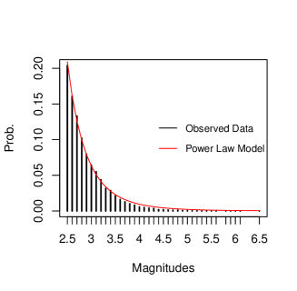
Figure 3: Probability density function of all the earthquakes registered from 16/04/2005 to 31/03/2017 with magnitudes not smaller than 2.5. The best fit of the empirical distribution with a power law of the type $y=ax^{b}$ is also shown. The calibrated parameters are $\hat{a}=86.32$ and $\hat{b}=-6.57$, with an $R^{2}$ of about 1.

Statistical Indicator	Value
Number of Data	13239
Maximum	6.50
Minimum	2.50
Mean ($\mu$)	2.88
Median ($m$)	2.80
RMS	2.91
Standard Deviation ($\sigma$)	0.42
Variance	0.18
Standard Error	0.002
Skewness	1.89
Kurtosis	8.24
$\mu/\sigma$	6.84
$3(\mu-m)/\sigma$	0.60

Table 2: Summary of the statistical characteristics for the magnitudes not smaller than 2.5 of the earthquakes occurred from April $16^{th}$, 2005 to March $31^{st}$, 2017.

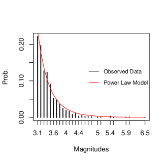
Figure 4: Probability density function of all the earthquakes registered in the provinces of Macerata, Perugia, Rieti, Ascoli Piceno, L’Aquila, Teramo, Terni and Fermo from January $24^{th}$, 2016 to January $24^{th}$, 2017, with magnitudes not smaller than 3.1. The best fit of the empirical distribution with a power law of the type $y=ax^{b}$ is also shown. The calibrated parameters are $\hat{a}=5805.79$ and $\hat{b}=-8.93$, with an $R^{2}$ of 0.98.

Statistical Indicator	Value
Number of Data	849
Maximum	6.50
Minimum	3.10
Mean ($\mu$)	3.42
Median ($m$)	3.30
RMS	3.44
Standard Deviation ($\sigma$)	0.39
Variance	0.15
Standard Error	0.01
Skewness	2.75
Kurtosis	15.05
$\mu/\sigma$	8.79
$3(\mu-m)/\sigma$	0.95

Table 3: Summary of the statistical characteristics for the magnitudes of the earthquakes with epicenters in the provinces of Macerata, Perugia, Rieti, Ascoli Piceno, L’Aquila, Teramo, Terni and Fermo from January $24^{th}$, 2016 to January $24^{th}$, 2017.

4 Results and discussion

Table 1 offers a preliminary view of the phenomenon under investigation. Since the empirical distribution of the sizes of the earthquakes can be well-fitted through a power law, as expected, the mean and the median of the magnitude distribution are different. This suggests the presence of asymmetry. The positional indicators show that the most part of the observations takes values close to 3.3. Furthermore, the variability indexes confirm that the values are rather concentrated near the distribution’s center. The positive skewness suggests a right-tailed shape, and the value of the kurtosis indicates a leptokurtic distribution. The leptokurtic property of the data is due to the presence of outliers (see Figure 2).
As mentioned above, the best fit procedures on (1) and (2) are performed over the dataset considering magnitudes not smaller than 3.1 for the reasons discussed in Section 1 and Section 3. Results are presented in Table 4 where the calibrated parameters and the $R^{2}$’s are reported. For a visual inspection of the goodness of fit, refer to Figures 5 and 6.

Eq. (1)	Calibrated parameter	Value
	$\hat{\alpha}$	6.21
	$\hat{\beta}$	0.00
	$\hat{\gamma}$	0.10
	$R^{2}$	0.98
Eq. (2)	Calibrated parameter	Value
	$\hat{k}$	8.63
	$\hat{\phi}$	0.00
	$\hat{\lambda}$	0.10
	$\hat{\psi}$	6972.72
	$\hat{\xi}$	0.04
	$R^{2}$	0.98

Table 4: Calibrated parameters of the best fit procedures, according to formulas (1) and (2) for the dataset with magnitude not smaller than 3.1 (N = 978; period: 24/01/2016 - 24/01/2017; Italy). The value of the $R^{2}$ in both of cases is reported.

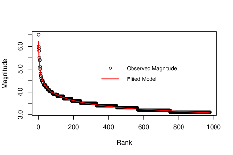
Figure 5: All the earthquakes with magnitude not smaller than 3.1 registered in Italy from 24/01/2016 to 24/01/2017 ranked by decreasing order according to their magnitude with the corresponding ZML fit. See formula (1).

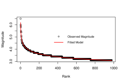
Figure 6: All the earthquakes with magnitude not smaller than 3.1 registered in Italy from 24/01/2016 to 24/01/2017 ranked by decreasing order according to their magnitude with the corresponding UL fit. See formula (2).

Eq. (1)	Calibrated parameter	Value
	$\hat{\alpha}$	9.48
	$\hat{\beta}$	68.80
	$\hat{\gamma}$	0.14
	$R^{2}$	0.98
Eq. (2)	Calibrated parameter	Value
	$\hat{k}$	0.88
	$\hat{\phi}$	9.52
	$\hat{\lambda}$	0.11
	$\hat{\psi}$	36951.95
	$\hat{\xi}$	0.30
	$R^{2}$	0.99

Table 5: Calibrated parameters of the best fit procedures, according to formulas (1) and (2) for the dataset built on an enlarged time window: April $16^{th}$, 2005 - March $31^{st}$, 2017 (N = 13239, magnitudes not smaller than 2.5). The value of the $R^{2}$ in both of cases is reported.

Figure 7: All the earthquakes registered from 16/04/2005 to 31/03/2017 with magnitudes not smaller than 2.5, ranked by decreasing order according to their magnitude with the corresponding ZML fit. See formula (1).

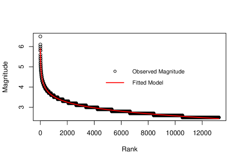
Figure 8: All the earthquakes registered from 16/04/2005 to 31/03/2017 with magnitudes not smaller than 2.5, ranked by decreasing order according to their magnitude with the corresponding UL fit. See formula (2).

Eq. (1)	Calibrated parameter	Value
	$\hat{\alpha}$	6.07
	$\hat{\beta}$	0.00
	$\hat{\gamma}$	0.10
	$R^{2}$	0.98
Eq. (2)	Calibrated parameter	Value
	$\hat{k}$	9.50
	$\hat{\phi}$	0.00
	$\hat{\lambda}$	0.10
	$\hat{\psi}$	6749.18
	$\hat{\xi}$	0.02
	$R^{2}$	0.98

Table 6: Calibrated parameters of the best fit procedures, according to formulas (1) and (2) for the dataset of the earthquakes occurred during the period: January $24^{th}$, 2016 to January $24^{th}$, 2017, with epicenters localized in the provinces of Macerata, Perugia, Rieti, Ascoli Piceno, L’Aquila, Teramo, Terni and Fermo, N = 849, magnitudes not smaller than 3.1. The value of the $R^{2}$ in both of cases is reported.

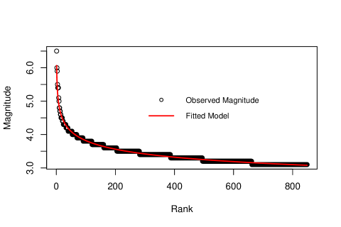
Figure 9: The earthquakes registered from 24/01/2016 to 24/01/2017 in the provinces of Macerata, Perugia, Rieti, Ascoli Piceno, L’Aquila, Teramo, Terni and Fermo, with magnitudes not smaller than 3.1, ranked by decreasing order according to their magnitude with the corresponding ZML fit. See formula (1).

Figure 10: The earthquakes registered from 24/01/2016 to 24/01/2017 in the provinces of Macerata, Perugia, Rieti, Ascoli Piceno, L’Aquila, Teramo, Terni and Fermo with magnitudes not smaller than 3.1, ranked by decreasing order according to their magnitude with the corresponding UL fit. See formula (2).

The analysis evidences a first important fact that is the presence of outliers at low ranks. They do not affect the performance of the fitting procedures with (1) or (2), and consequently we cannot note substantial discrepancies in using ZML or UL for the dataset containing the earthquakes from 24/01/2016 to 24/01/2017 in Italy.
Looking at Section 3, we can compare our results with those obtained for the global and the local datasets and check the coherence of our findings.
The local analysis excludes 149 observations with magnitudes mainly allocated in the high rank and only one of magnitudes around 5. The exclusions do not change too much the estimations, and the parameters and the $R^{2}$’s remain rather similar to those presented for the case of the original sample. Such a similarity appears to be more evident for the ZML fit, hence supporting that the UL approximates the data in a more convincing way and is more sensitive to data variation (see Tables 4 and 6). In particular, the upper side of Tables 4 and 6 shows a ZML best fit calibration with $\hat{\beta}$ close to zero and a small value of $\hat{\gamma}$ because the fitted model captures at the best the effect of the low ranks. Consequently, $\hat{\alpha}$ is close to the highest registered magnitude. Visual inspection is also appealing (see Figures 5 and 9 for the ZML case and Figures 6 and 10 for the UL case). This suggests the negligible presence of space effects in performing the rank-size analysis and computing the cost indicators.
The situation is notably different for the case of the dataset with enlarged time window (see Table 5). In this case, we observe an increment of the relative number of magnitudes at high ranks, hence leading to a calibration which is more distorted from the small magnitude events and loses representation capacity at lowest ranks, even in presence of some outliers at low ranks.
The opportunity to catch the effects of the lowest ranked outliers is due to $\psi$ in (2) (see Cerqueti and Ausloos, 2016) which increases in the case of sizes at low ranked magnitudes close to the medium ranked sizes. By comparing the levels of the parameter $\hat{\psi}$ from Tables 4, 6 and 5, one can observe the increment in the global case. Notice that a small value of $\hat{\psi}$ stands for a fit which can capture the high ranked data effect without flattering the part of the curve at a low rank. Moreover, the parameter $\phi$ in (2) acts in the same way of $\psi$, but to capture the effects of the lowest outliers. Thus, in presence of high ranked outliers the value of $\phi$ increases. Consistently with this idea, $\hat{\phi}$ is equal to 9.52 for the case of the enlarged time window and it is null in the other cases.
A slight improvement of the goodness of fit is shown by the $R^{2}$ of the enlarged case, even if it moves from 0.98 to 0.99. So, the goodness of fit is generally so high that a discrepancy between observed data and fit curves are not appreciable (see Figures 5, 7 and 9 for the ZML case and Figures 6, 8 and 10 for the UL case).
We also notice that the highest (lowest) level of the magnitudes estimated through (1) and (2), namely $\hat{Z}^{ZML}_{Max}$ and $\hat{Z}^{UL}_{Max}$ ($\hat{Z}^{ZML}_{Min}$ and $\hat{Z}^{UL}_{Min}$), respectively, adds further arguments for supporting the goodness of fit. In fact, we have found $\hat{Z}^{ZML}_{Max}=6.21$, $\hat{Z}^{UL}_{Max}=6.18$, $\hat{Z}^{ZML}_{Min}=3.07$ and $\hat{Z}^{UL}_{Min}=3.07$. For the maximum points curves are slightly below the maximum empirical observation of 6.5, while for minimum we have the same value very close to 3.1, hence suggesting an analogous behavior at the highest rank.
To sum up, we argue that the ZML and UL show similar behaviors in fitting the original catalog and the one associated to the local dataset, hence giving a substantial lack of space effects. The analysis of catalog with $M_{c}=2.5$ and wider time windows highlights that the UL fit is more appropriate to represent the data, even if the goodness of fit remains unchanged. Thus, data show an analogous regularity property in both of cases of short and long period, and this suggests that results provided for the original sample are robust to enlargement of the period. The incompleteness catalog problem has been faced in both of cases by truncating to a low level of magnitude, in accord to seismological literature.
For what concerns the economic costs indicators, some integrals can be easily computed in closed form, while other ones will be estimated. We have

$$\Gamma^{(ii)}_{ZML}=\int_{0}^{\bar{r}_{ZML}}\hat{\alpha}(r+\hat{\beta})^{-\hat{\gamma}}dr=\frac{\hat{\alpha}}{1-\hat{\gamma}}\left[(\bar{r}_{ZML}+\hat{\beta})^{1-\hat{\gamma}}-\hat{\beta}^{1-\hat{\gamma}}\right]$$ (5)

$$\begin{split}\Gamma^{(iii)}_{ZML}&=\int_{0}^{\bar{r}_{ZML}}\ln\left(\hat{\alpha}(r+\hat{\beta})^{-\hat{\gamma}}\right)dr=\ln\left(\hat{\alpha}\right)\cdot\bar{r}_{ZML}-\\ &-\hat{\gamma}\cdot\left[(\bar{r}_{ZML}+\hat{\beta})\{\ln(\bar{r}_{ZML}+\hat{\beta})-1\}-\hat{\beta}\{\ln(\hat{\beta})-1\}\right];\end{split}$$ (6)

$$\begin{split}\Gamma^{(iii)}_{UL}&=\int_{0}^{\bar{r}_{UL}}\ln\left(\hat{k}\cdot\dfrac{(N+1-r+\hat{\psi})^{\hat{\xi}}}{[N(r+\hat{\phi})]^{\hat{\lambda}}}\right)dr=\ln\hat{k}\cdot{\bar{r}_{UL}}+\\ &+\hat{\xi}\left[-(N+1-\bar{r}_{UL}+\hat{\psi})\{\ln(N+1-\bar{r}_{UL}+\hat{\psi})-1\}+(N+1+\hat{\psi})\{\ln(N+1+\hat{\psi})-1\}\right]-\\ &-\hat{\lambda}\cdot\left[\ln(N)\cdot\bar{r}_{UL}+(\bar{r}_{UL}+\hat{\phi})\{\ln(\bar{r}_{UL}+\hat{\phi})-1\}-\hat{\phi}\{\ln(\hat{\phi})-1\}\right].\end{split}$$ (7)

The other cases of cost indicators $\Gamma$s are properly estimated through standard numerical techniques. Specifically, the generic interval $[0,\bar{r}]$ is discretized in $S$ sub–intervals with a discretization step $\Delta r$, so that

$$r_{0}=0,\qquad r_{s}=r_{s-1}+\Delta r,\qquad r_{S}=\bar{r}.$$

From such a discretization, the generic integrals defining the $\Gamma$’s are approximated as follows:

$$\Gamma=\int_{0}^{\bar{r}}H(r)dr\sim\Delta r\cdot\sum_{s=1}^{S}H(r_{s}).$$

Now, recall that a specific value of $\bar{r}$ is associated to a value of $\bar{z}$. Thus, we can compare the cost indicators in terms of the threshold magnitudes $\bar{z}$.
Figure 11 allows the comparison among the cases of $\Gamma_{ZML}$’s and $\Gamma_{UL}$’s as $\bar{z}$ varies, respectively. The discretization step used for integral approximation in (5), (6) and (7) is taken as $\Delta r=$ 0.01.
Cost indicators are decreasing functions of $\bar{z}$, as expected. The value of $\bar{z}$ that represents a measure of the Italian infrastructures’ ability of resisting to earthquakes.
The costs decays have no differences in the behaviours considering the two fit functions (see Figure 11).
As expected, for both of cases of Eq. (1) and (2), the most expensive case emerges by transforming magnitudes into cost with the exponential function $\Gamma^{(i)}$, while the logarithmic transformation of the magnitudes leads to the lowest level of cost indicator and the sensitiveness to increments of $\bar{z}$ are less evident.
The $\Gamma^{(ii)}$’s and $\Gamma^{(iii)}$’s decay quite simultaneously, even if starting by different point, and converge to zero, while $\Gamma^{(i)}_{ZML}$ and $\Gamma^{(i)}_{UL}$ tend to rapidly reduce the cost until $\bar{z}$ is around 3.7 (by a visual inspection). After this threshold the curves’ inclination decrease very slowly denoting resistance to damages reduction.
Furthermore, the exponential transformations of estimated magnitude flatten after about $\bar{z}=3.5$.
Moreover, one can observe a change in the concavity of the curves $\Gamma^{(i)}$’s around magnitude 5.7. After such a value, the curves decrease rapidly to zero. This finding suggests that the aggregated economic costs of the earthquakes collapse rapidly above a large enough threshold, and this should be viewed as a hint to the policymakers of implementing strategies for letting the no-damage zone above such a magnitude threshold.
In order to visualize the robustness of the results obtained with this cost analysis, in Figures 12 and 13 we also present the different curves obtained from the different dataset presented in Section 3. Panel (a) is the case of the original sample, (b) is the local analysis and (c) is the global one.
For the cases of the cost indicators calibrated on the Eq. (1), see Figure 12. We can note that (a) and (b) have the same shapes, but (b) is a little bit scaled due to the fact that the zones individuated entails the exclusion of some seismic events. The decays are the same but the curves of the (b) case reach zero first. A motivation can be found in the exclusion of an important earthquake of magnitude around 5.5 in the local dataset, hence leading to slightly cheaper damages. Case (c) is referred to a wider time window (about 12 years) and to a dataset with $M_{c}=2.5$ on average. Consequently, as expected, the increased amount of minor earthquakes rises the cost mainly in the left side of the curve. In this case, null costs are achieved at magnitudes around 5.5. This misrepresentation is due to the functional form of ZML, being the percentage of high-magnitudes phenomena over the considered series very low.
The costs analysis performed with the employment of Eq. (2) are reported in Figure 13. For cases (a) and (b), the same arguments carried out above can be applied. The null costs are achieved for a magnitude in case (b) smaller than that of case (a), due to the removal of one important seismic event in the local dataset. The (c) case is different. There one can appreciate the relevant capacity of the UL in representing the data. In fact the zeroing of the costs occurs near magnitude 6.5, which is the real value of the highest registered earthquake.
To conclude, the definition of economic costs performed over the original sample (see Figures 12 and 13, panel (a)) can be reasonably considered valid because they coherently represent the logic of the phenomena that we are studying. Furthermore, the implemented selection of the local dataset does not change the substance of the findings, hence supporting the negligibility of space effects in the considered sample (see De Natale et al. (1988)). Furthermore, results are robust also in terms of the catalog incompleteness problem, in that taking magnitudes not smaller than 3.1 and 2.5 has a very weak effect on the total cost aggregation.

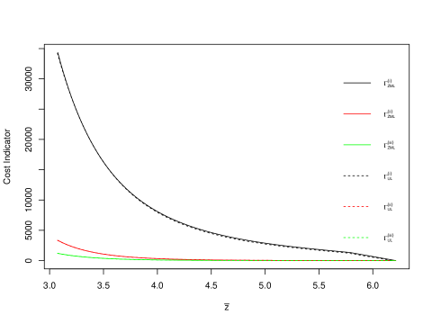
Figure 11: Comparison among $\Gamma^{(i)}_{ZML}$, $\Gamma^{(ii)}_{ZML}$, $\Gamma^{(iii)}_{ZML}$, $\Gamma^{(i)}_{UL}$, $\Gamma^{(ii)}_{UL}$ and $\Gamma^{(iii)}_{UL}$ as $\bar{z}$ varies. They are calibrated on the Italian earthquakes registered from 24/01/2016 to 24/01/2017 with magnitudes not smaller than 3.1

Figure 12: (a) Comparison among $\Gamma^{(i)}_{ZML}$, $\Gamma^{(ii)}_{ZML}$ and $\Gamma^{(iii)}_{ZML}$ as $\bar{z}$ varies. The case of earthquakes registered from 24/01/2016 to 24/01/2017 in Italy with magnitudes not smaller than 3.1 is presented.
(b) Comparison among $\Gamma^{(i)}_{ZML}$, $\Gamma^{(ii)}_{ZML}$ and $\Gamma^{(iii)}_{ZML}$ as $\bar{z}$ varies. The case of earthquakes registered from 24/01/2016 to 24/01/2017 in Macerata, Perugia, Rieti, Ascoli Piceno, L’Aquila, Teramo, Terni and Fermo Provinces (comprised the respective coasts) with magnitudes not smaller than 3.1 is presented.
(c) Comparison among $\Gamma^{(i)}_{ZML}$, $\Gamma^{(ii)}_{ZML}$ and $\Gamma^{(iii)}_{ZML}$ as $\bar{z}$ varies. The case of earthquakes registered from 16/04/2005 to 31/03/2017 in Italy with magnitudes not smaller than 2.5 is presented.

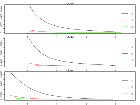
Figure 13: (a) Comparison among $\Gamma^{(i)}_{UL}$, $\Gamma^{(ii)}_{UL}$ and $\Gamma^{(iii)}_{UL}$ as $\bar{z}$ varies. The case of earthquakes registered from 24/01/2016 to 24/01/2017 in Italy with magnitudes not smaller than 3.1 is presented.
(b) Comparison among $\Gamma^{(i)}_{UL}$, $\Gamma^{(ii)}_{UL}$ and $\Gamma^{(iii)}_{UL}$ as $\bar{z}$ varies. The case of earthquakes registered from 24/01/2016 to 24/01/2017 in Macerata, Perugia, Rieti, Ascoli Piceno, L’Aquila, Teramo, Terni and Fermo Provinces (comprised the respective coasts) with magnitudes not smaller than 3.1 is presented.
(c) Comparison among $\Gamma^{(i)}_{UL}$, $\Gamma^{(ii)}_{UL}$ and $\Gamma^{(iii)}_{UL}$ as $\bar{z}$ varies. The case of earthquakes registered from 16/04/2005 to 31/03/2017 in Italy with magnitudes not smaller than 2.5 is presented.

5 Conclusions

This paper deals with a rank-size analysis of earthquakes’ magnitudes occurred in Italy from $24^{th}$ January, 2016 to $24^{th}$ January, 2017. Two different fit functions are proposed: the ZML (see Eq 1) and the UL (see Eq. 2). It is shown that the earthquakes data exhibit a strong rank-size regularity and that the both functions exhibit a remarkable goodness of fit.
The five parameters UL (2) improves the fit – even if in a not so significant way – only when an enlargement in time and magnitude of the dataset is implemented. In this case, UL is more capable than ZML to capture the effect of higher earthquakes.
To e consistent under a seismological perspective, both problems of incomplete catalog and of space effects have been treated.
Moreover, a new formulation of economic cost indicators has been introduced. Such a conceptualization moves from the presence of a critical threshold for the magnitude which distinguishes earthquakes in terms of damages.
The definition of economic costs performed over the original sample (see Figures 12 and 13, panel (a)) can be reasonably considered valid because they coherently represent the logic of the phenomena that we are studying. Furthermore, the implemented selection of the local dataset does not change the substance of the findings, hence supporting the negligibility of space effects in the considered sample (see De Natale et al. (1988)). Results are robust also in terms of the catalog incompleteness problem, in that taking magnitudes not smaller than 3.1 and 2.5 has a very weak effect on the total cost aggregation.
The analysis of the cost indicators explains clearly that the reduction of the earthquakes’ impact on infrastructures should be pursue by letting the no-damages magnitude growing (see Figures 11, 12 and 13). More than this, the discussion of three different scenarios for the individual cost of an earthquake with a given magnitude illustrates also the way in which such a reduction takes place. The obtained results suggest to adopt risk management strategies pointing at the mechanism of economic costs creation in terms of earthquake magnitudes.

References

- [1] Aguilar-San Juan, B., Guzman-Vargas, L., 2013. Earthquake magnitude time series: scaling behavior of visibility networks. European Physical Journal B 86, 454.
- [2] Amato, A., Mele, F.M., 2008. Performance of the INGV National Seismic Network from 1997 to 2007. Annals of Geophysics 51, 417-431.
- [3] Ausloos, M., Cerqueti, R., 2016. A universal rank-size law. PLoS ONE 11(11), e0166011.
- [4] Axtell, R.L., 2001. Zipf Distribution of U.S. Firm Sizes. Science 293(5536), 1818-1820.
- [5] Blasius, B., Tönjes, R., 2009, Zipf’s law in the popularity distribution of chess openings. Physical Review Letters 103(21), 218701.
- [6] Bottazzi, G., Pirino, D., Tamagni, F. 2015. Zipf law and the firm size distribution: a critical discussion of popular estimators. Journal of Evolutionary Economics 25(3), 585-610.
- [7] Cerqueti, R., Ausloos, M., 2015. Evidence of Economic Regularities and Disparities of Italian Regions From Aggregated Tax Income Size Data. Physica A: Statistical Mechanics and its Applications 421(1), 187-207.
- [8] Chiaraluce, L., Di Stefano, R., Tinti, E., Scognamiglio, L., Michele, M., Casarotti, E., Cattaneo, M., De Gori, P., Chiarabba, C., Monachesi, G., Lombardi, A., Valoroso, L., Latorre, D., Marzorati, S., 2017. The 2016 Central Italy Seismic Sequence: A First Look at the Mainshocks, Aftershocks, and Source Models. Seismological Research Letters, doi: 10.1785/0220160221.
- [9] Dimitrova, Z., Ausloos, M., 2015. Primacy analysis of the system of Bulgarian cities. Central European Journal of Physics 13, 218-225.
- [10] Fairthorne, R.A., 2005. Empirical Hypberbolic Distributions (Bradford-Zipf-Mandelbrot) for Bibliometric Description and Prediction. Journal of Documentation 61(2), 171-193.
- [11] Fujita, M., Krugman, P., Venables, A.J., 2001. The Spatial Economy: Cities, Regions, and International Trade. MIT Press, Cambridge, MA.
- [12] Fujita, M., Thisse, J.F., 2000. The formation of economic agglomerations: Old problems and new perspectives. Economics of Cities: Theoretical Perspectives, 3-73.
- [13] Fujiwara, Y. (2004). Zipf law in firms bankruptcy. Physica A: Statistical Mechanics and its Applications, 337(1), 219–230.
- [14] Gabaix, X., Ioannides, Y.M., 2004. The Evolution of City Size Distributions. Handbookof Regional and Urban Economics 4, 2341-2378.
- [15] Gruppo di Lavoro INGV sul Terremoto in centro Italia,2016. SUMMARY REPORT ON THE 30 OCTOBER, 2016 EARTHQUAKE IN CENTRAL ITALY 6.5. doi: 10.5281/zenodo.166238 .
- [16] Huang, S. M., Yen, D. C., Yang, L. W., Hua, J. S., 2008. An investigation of Zipf’s Law for fraud detection. Decision Support Systems 46(1), 70-83.
- [17] Ioannides, Y.M., Overman, H.G., 2003. Zipf’s law for cities: an empirical examination. Regional Science and Urban Economics 33(2), 127-137.
- [18] Ioannides, Y.M., Skouras, S., 2013. US city size distribution:robustly Pareto, but only in the tail. Journal of Urban Economics 73(1), 18-29.
- [19] Jaumé, S.C., 2000. Changes in Earthquake Size–Frequency Distributions Underlying Accelerating Seismic Moment/Energy Release. In: Geocomplexity and the Physics of Earthquakes (eds J. B. Rundle, D. L. Turcotte and W. Klein), American Geophysical Union, Washington, D.C.. doi: 10.1029/GM120p0199.
- [20] Kagan, Y.Y., 2010. Earthquake size distribution: Power-law with exponent ?. Tectonophysics 490(1), 103-114.
- [21] Lavalette, D., 1966. Facteur d’impact: impartialité ou impuissance. Internal Report, INSERM U350, Institut Curie, France.
- [22] Levenberg, K., 1944. A method for the solution of certain problems in least squares. Quarterly Applied Mathematics 2(2), 164-168.
- [23] Levene, M., Borges, J., Loizou, G., 2001. Zipf’s law for Web surfers. Knowledge and Information Systems 3(1), 120-129.
- [24] Li, W., Yang W., 2002. Zipf’s Law in Importance of Genes for Cancer Classification Using Microarray Data. Journal of Theoretical Biology 219(4), 539-551.
- [25] Lourakis, M. I., 2005. A brief description of the Levenberg-Marquardt algorithm implemented by levmar. Foundation of Research and Technology 4, 1-6.
- [26] Maillart, T., Sornette, D., Spaeth, S., von Krogh, G., 2008. Empirical Tests of Zipf’s Law Mechanism in Open Source Linux Distribution. Physical Review Letters 101(21), 218701.
- [27] Mandelbrot, B., 1953. An informational theory of the statistical structure of language. Communication theory 84, 486-502.
- [28] Mandelbrot, B., 1961. On the theory of word frequencies and on related Markovian models of discourse. Structure of language and its mathematical aspects 12, 190-219.
- [29] Manaris, B., Romero, J., Machado, P., Krehbiel, D., Hirzel, T., Pharr, W., Davis, R. B., 2005. Zipf’s law, music classification, and aesthetics. Computer Music Journal 29(1), 55-69.
- [30] Marchetti A., Ciaccio, M.G., Nardi, A., Bono, A., Mele, F.M., Margheriti, L., Rossi, A., Battelli, P., Melorio, C., Castello, B., Lauciani, V., Berardi, M., Castellano, C., Arcoraci, L., Lozzi, G., Battelli, A., Thermes, C., Pagliuca, N., Modica, G., Lisi, A., Pizzino, L., Baccheschi, P., Pintore, S., Quintiliani, M., Mandiello, A., Marcocci, C., Fares, M., Cheloni, D., Frepoli, A., Latorre, D., Lombardi, A.M., Moretti, M., Pastori, M., Vallocchia, M., Govoni, A., Scognamiglio, L., Basili, A., Michelini, A., Mazza, S., 2016. The Italian Seismic Bulletin: strategies, revised pickings and locations of the central Italy seismic sequence. Annals of Geophysics 59, doi: 10.4401/ag-7169.
- [31] Marquardt, D.W., 1963. An Algorithm for Least-Squares Estimation of Nonlinear Parameters. Journal of the Society for Industrial and Applied Mathematics 11(2), 431-441.
- [32] Matlaba, V.J., Holmes, M.J., McCann, P., Poot, J., 2013. A century of the evolution of the urban system in Brazil. Review of Urban and Regional Development Studies 25(3), 129-151.
- [33] Mega, M.S., Allegrini, P., Grigolini, P., Latora, V., Palatella, L., Rapisarda, A., Vinciguerra, S., 2003. Power-law time distribution of large earthquakes. Physical Review Letters 90(18), 188501.
- [34] Montemurro, A.M., 2001. Beyond the Zipf-Mandelbrot law in quantitative linguistics. Physica A: Statistical Mechanics and its Applications 300(3), 567-578.
- [35] Moretti, M., Pondrelli, S., Margheriti, L., Abruzzese, L., Anselmi, M., Arroucau, P., Baccheschi, P., Baptie, B., Bonadio, R., Bono, A., Bucci, A., Buttinelli, M., Capello, M., Cardinale, V., Castagnozzi, A., Cattaneo, M., Cecere, G., Chiarabba, C., Chiaraluce, L., Cimini, G.B., Cogliano, R., Colasanti, G., Colasanti, M., Criscuoli, F., D’Alema, E., D’Alessandro, A., D’Ambrosio, C., Danecek, P., De Caro, M., De Gori, P., Delladio, A., De Luca, G., De Luca, G., Demartin, M., Di Nezza, M., Di Stefano, R., Falco, L., Fares, M., Frapiccini, M., Frepoli, A., Galluzzo, D., Giandomenico, E., Giovani, L., Giunchi, C., Govoni, A., Hawthorn, D., Ladina, C., Lauciani, V., Lindsay, A., Mancini, S., Mandiello, A.G., Marzorati, S., Massa, M., Memmolo, A., Migliari, F., Minichiello, F., Monachesi, G., Montuori, C., Moschillo, R., Murphy, S., Pagliuca, N.M., Pastori, M., Piccinini, D., Piccolini, U., Pintore, S., Poggiali, G., Rao, S., Saccorotti, G., Segou, M., Serratore, A., Silvestri, M., Silvestri, S., Vallocchia, M., Valoroso, L., Zuccarello, L., Michelini, A., Mazza, S., 2016. SISMIKO: emergency network deployment and data sharing for the 2016 central Italy seismic sequence. Annals of Geophysics 59, doi: 10.4401/ag-7212.
- [36] De Natale, G., Musmeci, F., Zollo, A., 1988. A linear intensity model to investigate the causal relation between Calabrian and North-Aegean earthquake sequences. Geophysical Journal International 95(2), 285-293.
- [37] Newman, M.E., 2005. Power laws, Pareto distributions and Zipf’s law. Contemporary physics 46(5), 323-351.
- [38] Peng, G., 2010. Zipf’s law for Chinese cities: Rolling sample regressions. Physica A: Statistical Mechanics and its Applications 389(18), 3804-3813.
- [39] Piantadosi, S.T., 2014. Zipf’s word frequency law in natural language: A critical review and future directions. Psychonomic bulletin & review 21(5), 1112–1130.
- [40] Pinto, C.M., Lopes, A.M., Machado, J.T., 2012. A review of power laws in real life phenomena. Communications in Nonlinear Science and Numerical Simulation 17(9), 3558-3578.
- [41] Rosen, K.T., Resnick, M., 1980. The size distribution of cities: an examination of the Pareto law and primacy. Journal of Urban Economics 8(2), 165-186.
- [42] Romashkova, L., Peresan, A., 2013. Analysis of Italian earthquake catalogs in the context of intermediate-term prediction problem. Acta Geophysica 61(3), 583-610.
- [43] Saichev, A., Sornette, D., 2006. Power law distribution of seismic rates: theory and data analysis. European Physical Journal B 49, 377-401.
- [44] Schorlemmer, D., Mele, F., Marzocchi, W., 2010. A completeness analysis of the National Seismic Network of Italy, Journal of Geophysical Research 115, B04308, doi: 10.1029/2008JB006097.
- [45] Wu, Z.L., 2000. Frequency–size distribution of global seismicity seen from broad-band radiated energy. Geophysical Journal International 142(1), 59-66.
- [46] Zanette, D. H., 2006. Zipf’s law and the creation of musical context. Musicae Scientiae 10(1), 3-18.
- [47] Zipf, G.K., 1935. The Psychobiology of Language, Houghton-Mifflin.
- [48] Zipf, G.K., 1949. Human Behavior and the Principle of Least Effort.