Concurrent intersection point of magnetization and magneto-conductivity curves in strongly fluctuating superconductors

Abstract

The thermal fluctuations contribution to magnetization and magneto-conductivity of type II layered superconductor is calculated in the framework of Lawrence-Doniach model. For numerous high temperature cuprate superconductors, it was discovered that the magnetization dependence on temperature in wide range of fields exhibits an intersection point at a temperature slightly below $T_{c}$. We notice a similar intersection point of the magneto-conductivity curves at the approximate same temperature. The phenomenon is explained by strong (non-gaussian) thermal fluctuations with interactions treated using a self-consistent theory. All higher Landau levels should be included. Dimensionality of the fluctuations is defined and the 2D-3D dimensional crossover is the key for the existence of intersection points.

I Introduction

Discovery of high temperature superconductors (HTSC) attracted attention to effects of thermal fluctuations on the thermodynamic, magnetic and transport of type-II superconductors. In these materials, even at zero magnetic field, the role of thermal fluctuations is enhanced by several factors including high critical temperature, short coherence length and large anisotropy. Very large second critical magnetic field makes the highest available fields accessible for experiments in the superconducting states. Strong magnetic field greatly enhances the effect of the fluctuations making the magnetic phase diagram very complicated by creating the vortex liquid state over large range of temperatures below $T_{c}$ (clearly seen in magnetizationZeldov1995 and specific heatSchilling1997 ; Junod1999 ), and broadening the resistance drop in magneto-resistence upon transition.

More recently the fluctuations effects well above $T_{c}$ have been studied in detail for magnetizationLuLi2010 , electric conductivityRullier2011 , and Nernst effectXu2000 ; Wang2006 . The magnitude of thermal fluctuation is quantified by the Ginzburg number $Gi$, which can reach $10^{-2}$-$10^{-1}$ in high-$T_{c}$ cuprate superconductors in contrast with $10^{-9}$-$10^{-6}$ for conventional low-$T_{c}$ superconductors. In other unconventional superconductors like pnictides the fluctuations are still very significant. Though the multi-band structure of the iron-based superconductors is different from cuprate superconductors, they show many similarities like the two dimensional layered-structure.

If a superconductor is strongly fluctuating, “virtual” or “preformed” Cooper pairs exist above $T_{c}$, but the order parameter $\Psi$ is not phase coherent. Average of its amplitude (related to the superfluid density- $\left\langle\left|\Psi\right|^{2}\right\rangle$) might be sufficiently large to dominate electromagnetic properties like magnetization and magneto-transport over the typically small normal background.

When magnetization was measured, it was found surprisingly that, when the magnetization as a function of temperature, $M\left(T\right)$, plotted at different magnetic fields $H$, the curves intersect at the same temperature $T^{\ast}$. The first clear demonstration of this observation in $YBa_{2}Cu_{3}O_{7-\delta}$ ($YBCO$) Welp1991 and $Bi_{2}Sr_{2}CaCu_{2}O_{8}$ ($BSCCO$) Kes1991 has been made in early nineties, and later extended to $Tl_{2}Ba_{2}CaCu_{2}O_{8}$ ($TBCCO$) Wahl1997 , $HgBa_{2}Ca_{2}Cu_{3}O_{8+\delta}$ ($HgBCCO$) Naughton2000 and $La_{2-x}Sr_{x}CuO_{4+\delta}$ ($LSCO$) Finnemore2002 . The physics in the relevant part of the magnetic phase diagram is that of the vortex liquid. The basic vortex liquid theory was developed in eightiesThouless1975 ; Thouless1976 based on the idea of a homogeneous state with finite correlation determined by the energy gap $\varepsilon$ characterizing short range order. Typically the energy gap is estimated theoretically in a self - consistent manner.

Over the years there have been several attempts to explain the appearance of the intersection point of the magnetization curves. First the theory was restricted (due to complexity of a nonperturbative problem) to the lowest Landau level (LLL). The restriction allowed to obtain nonperturbative expressions even in the strongly fluctuating cases both in 2D and 3D, seeTesanovic1994, and references therein. Bulaevskii et alBulaevskii1992 attempted to use the 2D version of the theory to explain the intersection point in $YBCO$, however it was subsequently realized that the exact intersection is inconsistent with the strict LLL scalingRosenstein2005 .

When the restriction on the first Landau level was liftedJiang2014 (while still retaining the self-consistent fluctuation theory of the vortex liquid), the Ginzburg Landau (GL) theory extended to layered materials became capable to describe magnetization in $LSCO$, $BSCCO$ and $YBCO$ in wide range of fields and temperatures (even above $T_{c}$) with small number of parameters. Both experimentally and theoretically it became apparently that the intersection point is never exact. It depends slightly on magnetic field in surprisingly wide range of fields, but beyond this range the phenomenon quickly disappears.

An interesting question arises whether the similar “intersection point” also appears in other fluctuation phenomena like fluctuation transport, for example, the magneto-resistance. Ullah and DorseyDorsey1991 obtained expressions for the scaling behavior as a function of magnetic field and temperature of various thermodynamic and transport quantities within the self-consistent Hartree approximation and under the LLL restriction. They demonstrated that the product of the superconducting part of conductivity $\sigma_{s}$ (due to the order parameter) and magnetic field,  $K\equiv\sigma_{s}H$, scales exactly as the magnetization $M$ in the LLL restriction. The 3D LLL scaling in part of magnetic phase diagrams was later confirmed experimentallyWelp1991 in optimally doped $YBCO$ and later in other cupratesLan1993 ; Kim1992 and pnictidesPallecchi2009 ; Liu2010 . As a consequence, one would expect intersection points for $K$. We therefore have replotted $K$ as function of temperature for $YBCO$Palstra1989 , see Fig.1, and one iron pnictide superconductor, $LaFeAsO_{0.9}F_{0.1-\delta}$Chen2008 discussed below. The curves intersect approximately at the same temperature $T^{\ast}$ for different magnetic fields $H$.

As the vortex pinning is the mechanism for the existing of superconducting states in type II superconductors and therefore it might can not be ignored. However the intersection point region is close to the critical temperature, and in highly fluctuating superconductors (large Ginzburg number), due to strong thermal fluctuation the pinning effect for vortex liquid is very small due to thermal de-pinning. Therefore the pinning and the pair breaking scattering due to pinning can be ignored in this paper.

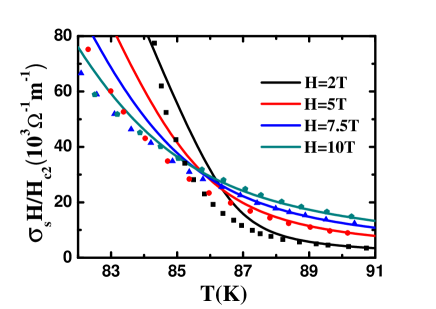
Figure 1: The intersection points of conductivity times magnetic field vs temperature $T$ of $YBCO$.

In this paper we present a quantitative theory of magnetization and magneto - conductivity and explain the intersection points within the phenomenological GL framework. It turns out that the layered structure, determining the dimensionality of the thermal fluctuations, is crucial for the appearance of the concurrent intersection points of various physical quantities, so the Lawrence Doniach (LD) model should be used. The calculation of conductivity requires the time dependent version of the model. The same sufficiently precise self - consistent method in the vortex liquid phase should be used to obtain simultaneously magnetization and conductivity.

The formulas of the magnetization and conductivity are used to fit the experimental data of various materials. It turns out that $T^{\ast}$ is located in the 2D - 3D crossover temperature regime in which the coherence length $\xi_{c}\left(T\right)$ in the direction perpendicular to the layers is roughly equal to the interlayer spacing.

The paper is organized as follows. The theoretical calculation of fluctuation magnetization and conductivity based on the LD model and time dependent Ginzburg Landau (TDGL) theory are introduced in Sec. II. The intersection points of fluctuation magnetization is calculated in Sec. III. The intersection points of conductivity curves of cuprate superconductors and pnictide superconductors are discussed in Sec. IV. We conclude in Sec. V. that the intersection points of magnetization and conductivity are due to the 2D-3D dimensional crossover.

II Fluctuation magnetization and conductivity in the Lawrence - Doniach model.

II.1 Model

The Lawrence-Doniach model are used to study the vortex matter in layered superconductors in the Ginzburg - Landau phenomenological approach. The Ginzburg - Landau free energy is expressed in terms of complex order parameter $\Psi_{n}\left(\mathbf{r}\right)$ in the $n$-th superconducting layer:

$$F_{GL} = d^{\prime}\sum_{n}\int d\mathbf{r}\left[\frac{\hbar^{2}}{2m^{\ast}}\left|\mathbf{D}\Psi_{n}\right|^{2}+\frac{\hbar^{2}}{2m_{c}d^{\prime 2}}\left|\Psi_{n}-\Psi_{n+1}\right|^{2}\right.$$ (1)

$$\left.+\alpha\left(T-T_{\Lambda}\right)\left|\Psi_{n}\right|^{2}+\frac{\beta}{2}\left|\Psi_{n}\right|^{4}\right]\text{.}$$

Here $\mathbf{r}$ is position in the superconducting plane. The second term describes the Josephson coupling between the planes separated by the inter-layer distance $d^{\prime}$. Applied field is assumed to be perpendicular to the planes and much larger that the lower critical field $H_{c1}$ so that in the vortex liquid phase the magnetic induction $B$ is homogeneous and magnetization is small compared to it. Therefore the vector potential in Landau gauge in the covariant derivative, $\mathbf{D=\nabla+}i\left(2e/\hbar c\right)\mathbf{A}$, can be approximated by $\mathbf{A=}\left(-By,0\right)$.

Parameters are as follows. The effective mass of a Cooper pair in the $a$-$b$ plane is $m^{\ast}$, while the one along the $c$ axis is $m_{c}$, so that the anisotropy parameter is $\gamma=\sqrt{m_{c}/m^{\ast}}$. The mean-field critical temperature in Eq.(1) is denoted by $T_{\Lambda}$ to stress its dependence on the ultraviolet cutoff $\Lambda$ (of the order of inverse lattice spacing). Thermal fluctuations of the order parameter on the mesoscopic scale, described by a Boltzmann sum, are generally characterized by the dimensionless 3D Ginzburg number,

$$Gi=\frac{1}{2}\left(\frac{8e^{2}\kappa^{2}\xi_{\Lambda}T_{c}\gamma}{\hbar^{2}c^{2}}\right)^{2}\text{.}$$ (2)

The Ginzburg-Landau parameter $\kappa$ is the ratio of the penetration depth, $\lambda_{\Lambda}=\frac{c}{2e^{\ast}}\sqrt{\frac{m^{\ast}\beta}{\pi\alpha T_{\Lambda}}}$, and the in - plane coherence length, $\xi_{\Lambda}=\hbar/\sqrt{2m^{\ast}\alpha T_{\Lambda}}$, and $T_{c}$ is the critical temperature.

To study the transport properties of a layered superconductor, the time dependent Ginzburg Landau Lawrence-Doniach model is used in a magnetic field near the mean-field transition temperatureHohenberg1977 :

$$\frac{\hbar^{2}\gamma_{D}}{2m}D_{\tau}\Psi_{n}=-\frac{1}{d^{\prime}}\frac{\delta F_{GL}}{\delta\Psi_{n}^{\ast}}+\zeta_{n}\text{.}$$ (3)

Here $D_{\tau}\equiv\partial/\partial_{\tau}-i\left(e^{\ast}/\hbar\right)\phi$ is the covariant time derivative with $\phi=-Ey$ being the scalar potential describing the electric field $E$ applied along the $y$ direction. The thermal noise term $\zeta_{n}$ should satisfy the fluctuation-dissipation theorem and ensure that the system relaxes to the proper equilibrium distribution,

$$\left\langle\zeta_{m}^{\ast}\left(\mathbf{r},\tau\right)\zeta_{n}\left(\mathbf{r}^{\prime},\tau^{\prime}\right)\right\rangle=\frac{\hbar^{2}\gamma_{D}}{m^{\ast}d^{\prime}}T\delta_{m,n}\delta\left(\mathbf{r-r}^{\prime}\right)\delta\left(\tau-\tau^{\prime}\right)\text{,}$$ (4)

where the $\left\langle\cdots\right\rangle$ denotes a thermal average.

II.2 Static properties of the vortex liquid phase within the self - consistent approximation.

The self - consistent fluctuation approximation (SCFA) in statics has been used to derive the magnetization in the vortex liquid phase in Ref. Jiang2014, in which the full derivations of the magnetization formula used below can be found. The basic characteristics of the vortex liquid is the excitation energy gap, which will be denoted by $\varepsilon$ in physical energy unit $\frac{2\hbar eH_{c2}}{m^{\ast}c}$($H_{c2}=\hbar c/2e\xi_{\Lambda}^{2}$ is the upper critical field). It is determined by the gap equation

$$\varepsilon = -a_{h}-\frac{\omega t}{\pi}\ln\left(1+\Lambda d^{2}+\sqrt{2\Lambda d^{2}+\Lambda^{2}d^{4}}\right)$$ (5)

$$+\frac{\omega td}{2\pi^{2}}\int_{k_{z}=0}^{2\pi/d}\left[\psi\left(g\left(k\right)+\Lambda/b\right)-\psi\left(g\left(k\right)\right)\right]\text{,}$$

where $k$ is the wave vector along the magnetic field direction and $\Lambda$ is the dimensionless cutoff energy in physical energy unit. The dimensionless “distance” from the $H_{c2}$ line is $a_{h}=\left(1-t-b\right)/2$, where $t=T/T_{c}$, $b=B/H_{c2}$ . The parameter $\omega$ describes the thermal fluctuation strength of the layered superconductors often expressed via the Ginzburg number, Eq.(2),

$$\omega=\frac{\pi}{d}\sqrt{2Gi}\text{.}$$ (6)

where $\Gamma$ and $\psi$ are the gamma and the digamma functions respectively and dimensionless layer distance is $d=d^{\prime}\gamma/\xi_{\Lambda}$. It is convenient to introduce a function of the perpendicular wave vector $k$ frequently used in the equations below,

$$g\left(k\right)=\frac{1}{b}\left(\frac{1-\cos kd}{d^{2}}+\varepsilon\right)\text{.}$$ (7)

The critical temperature $T_{c}$ is often smaller than the meanfield critical temperature $T_{\Lambda}$ due to strong thermal fluctuations on the mesoscopic scaleJiang2014 . Within the gaussian approximation the relation is given by

$$T_{c}=T_{\Lambda}\left[1-\frac{2\omega}{\pi}\ln\left(1+\Lambda d^{2}+d\sqrt{2\Lambda+\Lambda^{2}d^{2}}\right)\right]\text{.}$$ (8)

Magnetization was calculated in the framework of SCFA including all Landau levelsJiang2014 :

$$M = -\frac{2eT}{hcd^{\prime}}\left\{\frac{\Lambda}{b}+\frac{d}{2\pi}\int_{k}\left[\ln\Gamma\left(g\left(k\right)+\frac{\Lambda}{b}\right)\right.\right.$$ (9)

$$-\left(g\left(k\right)+\frac{\Lambda}{b}-\frac{1}{2}\right)\psi\left(g\left(k\right)+\frac{\Lambda}{b}\right)$$

$$\left.\left.+\left(g\left(k\right)-\frac{1}{2}\right)\psi\left(g\left(k\right)\right)-\ln\Gamma\left(g\left(k\right)\right)\right]\right\}\text{.}$$

Dynamical properties of the vortex liquid require the time dependent equation Eq.(3) involving an extra parameter, the diffusion constant $\gamma_{D}$.

II.3 Conductivity within the self - consistent approximation.

While for a BCS superconductor the diffusion constant $\gamma_{D}$ is related to parameters in GL model by $\gamma_{BCS}=\frac{\pi\hbar}{8T_{\Lambda}\xi_{\Lambda}^{2}}$, for unconventional superconductors, this relation can be modified, $\gamma_{D}=\eta\gamma_{BCS}$ ($\eta$ is a fitting parameter of order $1$).

The magneto conductivity of the layered superconductor due to superconducting fluctuation in the vortex liquid phase using SCFA was studied in Refs. Bui2010, ; Wang2016, , including high Landau levels. The Cooper pair contribution to the conductivity in terms of the excitation energy $\varepsilon$, determined by the gap equation Eq.(5), is

$$\sigma_{s} = \frac{e^{2}t\eta\gamma}{8hb\xi_{\Lambda}}\int_{k}\left\{\left(2g\left(k\right)-1\right)\left[\psi\left(g\left(k\right)\right)+\psi\left(g\left(k\right)+\frac{\Lambda}{b}+\frac{1}{2}\right)\right.\right.$$ (10)

$$\left.\left.-\psi\left(g\left(k\right)+\frac{1}{2}\right)-\psi\left(g\left(k\right)+\frac{\Lambda}{b}\right)\right]+\frac{\Lambda}{\Lambda-b/2+g\left(k\right)b}\right\}\text{.}$$

The detailed derivation of Eq.(10) can be found in Wang2016, . Having expressed both the static and the dynamical physical quantities within the same approximation, we now can turn to the main point of the present study: the intersection points at different magnetic fields. Let us start with magnetization.

III Intersection points of magnetization curves

As mentioned in Introduction, the intersection points for the magnetization, defined as,

$$\left.\frac{\partial M}{\partial H}\right|_{T=T^{\ast}}=0\text{,}$$ (11)

were measured in many high $T_{c}$ cuprates Salem09 ; Rosenstein2001 ; Naughton2000 ; Finnemore2002 and explained within the “lowest Landau level” approximation Bulaevskii1992 ; Rosenstein2005 . To calculate the intersection curve determined by Eq.(11) from Eq.(9), the derivative of magnetization with respect to the magnetic field is required,

$$\frac{\partial M}{\partial b} = -\frac{eT\gamma}{\pi hc\xi_{\Lambda}b}\int_{k}\left[-\left(g\left(k\right)+\frac{\Lambda}{b}-\frac{1}{2}\right)\left(\varepsilon_{b}^{\prime}-g\left(k\right)-\frac{\Lambda}{b}\right)\psi^{\prime}\left(g\left(k\right)+\frac{\Lambda}{b}\right)\right.$$ (12)

$$\left.+\left(g\left(k\right)-\frac{1}{2}\right)\psi^{\prime}\left(g\left(k\right)\right)\left(\varepsilon_{b}^{\prime}-g\left(k\right)\right)-\frac{\Lambda}{b}\right]\text{.}$$

Here the derivative $\varepsilon_{b}^{\prime}=\partial\varepsilon/\partial b$, that can be calculated using the gap equation, Eq.(5), and the intersection curve $T^{\ast}\left(H\right)$ is obtained numerically.

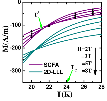
Figure 2: Magnetization data of Ref. LuLi2010, and theoretical fits(purple lines) of $LSCO$ crystal for various values of $H$. The comparison between the fluctuation magnetization calculated using the self-consistent fluctuation approximation (SCFA) vs the 2D lowest Landau level(2D-LLL) one.

In Fig. 2 magnetization curves of the under - doped$\ La_{1.91}Sr_{0.09}CuO_{4}$ ($T_{c}=24K$, $d^{\prime}=6.58\mathring{A}$) at $H=2T$, $3T$, $5T$, $8T$ fitted by Eq.(9) (purple lines) are shown. The fitting parametersJiang2014 are $H_{c2}=31T$, $\gamma=29$, $\Lambda=0.3$, $Gi=0.033$ and $\omega=0.138$. The result of SCFA approximation with all Landau level approach fits well with experiments (points). The magnetization in 2D-LLL approximation (detailed derivations are presented in Appendix A) is also shown in Fig. 2 (green lines). The 2D-LLL approximation theory predicts a single intersection point in contrary to the experimental data. Furthermore, it gave too big diamagnetization (roughly twice) compared to the SCFA result.

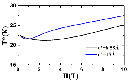
Figure 3: The intersection point lines $T^{\ast}\left(H\right)$ of magnetization vs magnetic fields $H$ for different interlayer spacing $d^{\prime}$ of $LSCO$ crystal.

In Fig.3, the intersection point lines $T^{\ast}\left(H\right)$ of two superconductors with different interlayer spacings are given. The first is underdoped $LSCO$ with $d^{\prime}=6.58\mathring{A}$ while the second (hypothetical) has $d^{\prime}=15\mathring{A}$ and all the other parameters, $T_{c}$, $H_{c2}$, $Gi$, $\gamma$, the same. For the first material, $T^{\ast}$ is nearly independent of magnetic field in the range $1T$ to $5T$ ($T^{\ast}\left(1T\right)=21.64K$, $T^{\ast}\left(2T\right)=21.27K$, $T^{\ast}\left(3T\right)=21.25K$, $T^{\ast}\left(4T\right)=21.5\ K$, $T^{\ast}\left(5T\right)=21.93K$). The best intersection point is at $21.4K$. For the hypothetical more anisotropic material, $T^{\ast}$ exhibits stronger dependence on $H$. Therefore in the $2D$ limit, there is no well defined intersection point. Since the earlier explanation of the intersection pointBulaevskii1992 ; Rosenstein2005 made use of 2D limit and LLL approximation, let us clarify why it is not likely.

Figure 4: The $\varepsilon\left(b\right)/b$ as function of magnetic field with fixed $d^{\prime}$=6.58Å and $T^{\ast}=21.4$K of $LSCO$ crystal.

In Fig.4 the energy gap of the vortex liquid, $\varepsilon\left(b\right)/b$, in underdoped $LSCO$ at $T^{\ast}=21.4K$ is given as a function of magnetic field. The LLL approximation condition $\varepsilon\left(b\right)<<b$ is questionable since $\varepsilon\left(b\right)/b$ exceeds $0.25$. So one has to look for an explanation elsewhere. An alternative is the dimensional 2D - 3D crossover taking place when coherence length in direction perpendicular to layers becomes comparable to the interlayer distance.

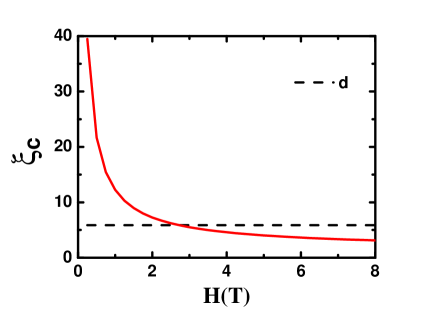
Figure 5: $\xi_{c}\left(H\right)$ as the function of magnetic field with fixed $d^{\prime}=6.58$Å ($d=5.87$) and $T^{\ast}=21.4$K of $LSCO$ crystal.

The correlation length $\xi_{c}$ is calculated in the Appendix. B. In Fig.5, it is shown for underdoped $LSCO$ at $T^{\ast}$ as a function of magnetic field. One notices that $\xi_{c}\left(H\right)=d^{\prime}$ at $H=2.7T$ just at the point in which the intersection point is defined the best (see a minimum in Fig.3). To conclude, the intersection points lies near the 2D - 3D crossover. This is one of the main results of the present paper.

The quantity $K$ shows also intersection point as it will be shown below. The definition of the intersection point for this quantity is

$$\left.\frac{\partial}{\partial H}K\right|_{T=T^{\ast}}=0\text{.}$$ (13)

The derivative of $K$ with respect to $b$ simplifies to

$$\frac{\partial K}{\partial b} = \frac{et\eta\gamma c}{32\pi b\xi_{\Lambda}^{3}}\int_{k}\left\{2\left(\varepsilon_{b}-g\left(k\right)\right)\left[\psi\left(g\left(k\right)+\frac{\Lambda}{b}+\frac{1}{2}\right)-\psi\left(g\left(k\right)+\frac{\Lambda}{b}\right)+\psi\left(g\left(k\right)\right)-\psi\left(g\left(k\right)+\frac{1}{2}\right)\right]\right.$$ (14)

$$+\left(2g\left(k\right)-1\right)\left[\left(\varepsilon_{b}-g\left(k\right)-\frac{\Lambda}{b}\right)\left(\psi^{\prime}\left(g\left(k\right)+\frac{\Lambda}{b}+\frac{1}{2}\right)-\psi^{\prime}\left(g\left(k\right)+\frac{\Lambda}{b}\right)\right)\right.$$

$$\left.+\left.\left(\varepsilon_{b}-g\left(k\right)\right)\left(\psi^{\prime}\left(g\left(k\right)\right)-\psi^{\prime}\left(g\left(k\right)+\frac{1}{2}\right)\right)\right]-\frac{\Lambda b\left(\varepsilon_{b}-1/2\right)}{\left(\Lambda+\left(g\left(k\right)-1/2\right)b\right)^{2}}\right\}\text{.}$$

Combining Eq.(14) and Eq.(13) the intersection point $T^{\ast}\left(H\right)$ is obtained. Detailed comparison with data follows.

Table 1: Fitting parameters for $YBa_{2}Cu_{3}O_{7}$, $LaFeAsO_{0.9}F_{0.1-\delta}$.

Material	$T_{c}$($K$)	$d^{\prime}(\mathring{A})$	$H_{c2}$($T$)	$\gamma$	$\Lambda$	$Gi$	$\omega$	$k$
$YBCuO$	$87.5$	$11.68$	$200$	$7.5$	$0.30$	$0.0011$	$0.022$	$1.4$
$LaFeAsO$	$20$	$8.717$	$50$	$7.64$	$0.30$	$0.0015$	$0.066$	$0.7$

YBCO. Magneto - resistivity data of $YBa_{2}Cu_{3}O_{7}$ ($T_{c}=87.5K$) single crystal of Ref. Palstra1989, is used to analyse the intersection points of $K$. The superconducting fluctuations component of the magneto - conductivity is obtained by subtracting the normal part, $\sigma_{s}=1/\rho-1/\rho_{n}$. The normal state resistivity $\rho_{n}$ in the low temperature region is given by the linear extrapolation of the resistivity curve from the high temperature region. The experimental data $\sigma_{s}H/H_{c2}$ as a function of temperature for various magnetic fields of $YBa_{2}Cu_{3}O_{7}$ ($T_{c}=87.5K$) single crystalPalstra1989 is shown in Fig.1. The experimental curves intersect roughly at a point between $5T$ to $10T$, and $T^{\ast}=85.8K$ is just below the critical temperature $T_{c}$. We use Eq.(5) and Eq.(10) to fit the data and the fitting parameters are listed in Table I (the interlayer distance $d^{\prime}=11.68\mathring{A}$ is taken from Ref. Poole2007, ). The solid curves are plotted using the fitting parameters. The curves fit very well in the high temperature region above $T^{\ast}=85.8K$, but the fitting in the low temperature region is not good. The reason can be attributed to pinning, whose influence on the conductivity becomes significant in the low temperature region.

The energy gap $\varepsilon\left(b\right)/b$ at $T^{\ast}=85.8K$ is shown in Fig.6. The curve varies approximately from $0.2$ to $0.3$ for $5T$ to $10T$. Therefore the LLL approximation is questionable in the intersection point region.

Figure 6: The $\varepsilon\left(b\right)/b$ as function of magnetic field with fixed $d^{\prime}$=11.68Å and $T^{\ast}=85.8$K of $YBCO$ crystal.

Fig.7 shows the coherence length dependence on the magnetic field at $T^{\ast}=85.8K$. $\xi_{c}\left(H\right)$ is quite near the interlayer distance between $5T$ to $10T$ (good intersection point region). Hence the appearance of intersection point is in the $2D-3D$ crossover region.

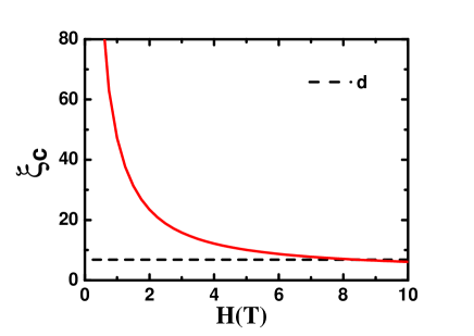
Figure 7: $\xi_{c}\left(H\right)$ as the function of magnetic field with fixed $d^{\prime}$=11.68Å and $T^{\ast}=85.8$K of $YBCO$ crystal.

Both the intersection curves for magnetization $M$ and conductivity $K$ are plotted in Fig.8. There are quite small differences for the two curves, and this means that the appearance of intersection points for $M$ and $K$ is due to the same physical mechanism.

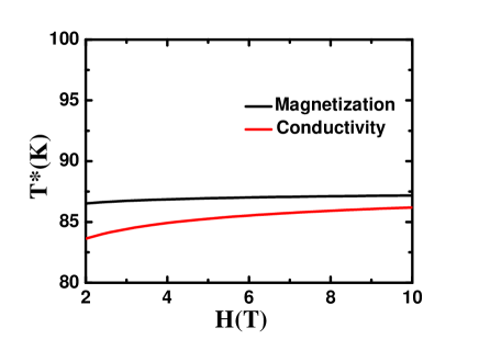
Figure 8: The comparison of intersection point lines between magnetization and conductivity of $YBCO$ crystal.

Pnictides. For Fe-based superconductors, the intersection points shall appear as they are mostly layered materials as well. The strongly layered, $LaFeAsO_{0.9}F_{0.1-\delta}$ ($T_{c}=20K$)Chen2008 with the anisotropy parameter $\gamma=7.64$ is considered. In Fig. 9, $\sigma_{s}H/H_{c2}$ vs $T$ for various magnetic fields studied is shown for $LaFeAsO$. The fitting parameters $\gamma$, $\omega$, $H_{c2}$ had been already established in Ref. Wang2016, and are listed in Table I.

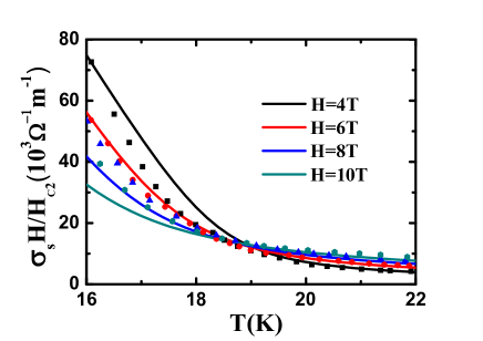
Figure 9: Intersection points in conductivity curves of LaFeAsO_0.9F_0.1-δ ($T_{c}=20$K)

IV Summary and Conclusions

To summarize, we noticed that in strongly fluctuating layered type II superconductors in the vortex liquid phase, the product of the superconducting part of conductivity $\sigma_{s}$ and of magnetic field, $K=\sigma_{s}H$, as a function of temperature has an “intersection point” similar to that noticed long ago in magnetization curves. To explain the intersection point phenomena, the self-consistent approximation theory of the Lawrence - Doniach model was adapted to calculate both quantities within the same framework.

The underdoped$\ LSCO$ and optimally doped $YBCO$ high $T_{c}$ cuprates are used as a test cases. $Fe$-based layered superconductor $LaFeAsO_{0.9}F_{0.1-\delta}$ Chen2008 demonstrates the existence of the intersection point phenomenon beyond cuprates. While in the past the “intersection points” were attributed to the 2D like superconducting fluctuation on the basis of the lowest Landau level theory of the vortex liquid phaseBulaevskii1992 , it was demonstrated that the LLL is not valid near the intersection point. For magnetization the value of 2D-LLL approximation is much larger than the SCFA one and these two temperature of intersection point is not equal, so that higher Landau levels must be taken into account.

The main observation is that the intersection point $T^{\ast}$, when it is well defined, is located in the vicinity of the 2D - 3D fluctuation crossover where the coherence length $\xi_{c}\left(T\right)$ in the direction perpendicular to the layers is approaching the interlayer spacing. Its location is not fixed, but changes moderately with magnetic field.

Acknowledgments.

We are grateful to Rui Wang and Professor V. M. Krasnov for valuable discussions. B.R. was supported by NSC of R.O.C. Grants No. 103-2112-M-009-014-MY3. The work of D.L. also is supported by National Natural Science Foundation of China (No. 11674007). B.R. is grateful to School of Physics of Peking University and Bar Ilan Center for Superconductivity for hospitality.

Appendix A 2D-LLL approximation of magnetization

Since the intersection points appear when the magnetic field is small compared to $H_{c2}$ and temperature does not deviate too far from $T_{c}$, let us simplify the expression, Eq.(9) for $b,\varepsilon\ll\Lambda$. It takes a form

$$M=-\frac{eT\gamma}{\pi hc\xi_{\Lambda}}\int_{k}\left\{\left(g\left(k\right)-1/2\right)\left(\psi\left(g\left(k\right)\right)-1\right)-\ln\frac{\Gamma\left(g\left(k\right)\right)}{\sqrt{2\pi}}\right\}\text{.}$$ (15)

The gap equation also simplifies:

$$\varepsilon=-a_{h}-\frac{\omega t}{\pi}\left[\ln\left(2bd^{2}\right)+\frac{d}{2\pi}\int_{k}\psi\left(g\left(k\right)\right)\right]\text{.}$$ (16)

In the LLL approximation, the inter Landau energy is much larger than the intra Landau level excitation, that is $b\gg\varepsilon$. The magnetization formula of Eq.(15) is

$$M_{LLL}=-\frac{eT}{hcd^{\prime}}\frac{b}{\sqrt{\varepsilon_{LLL}\left(2/d^{2}+\varepsilon_{LLL}\right)}}$$ (17)

with

$$\varepsilon_{LLL}=-a_{h}+\frac{\omega t}{\pi}\frac{b}{\sqrt{\varepsilon_{LLL}\left(2/d^{2}+\varepsilon_{LLL}\right)}}$$ (18)

By taking both the 2D and the LLL approximation, the intersection point can be found analytically. Taking the $d\rightarrow\infty$ limit of Eq.(17), one obtains,

$$M_{LLL}^{2D}\simeq-\frac{eT}{hcd^{\prime}}\frac{b}{\varepsilon_{LLL}^{2D}}\text{,}$$ (19)

where the gap equation for $\varepsilon_{LLL}^{2D}$ within the 2D-LLL approximation becomes just

$$\varepsilon_{LLL}^{2D}\simeq-a_{h}+\frac{\omega t}{\pi}\frac{b}{\varepsilon_{LLL}^{2D}}\text{.}$$ (20)

Using these expressions, the intersection point condition, Eq.(11), allows an analytic solution:

$$T_{LLL}^{2D\ast}=\frac{T_{c}}{1+4\omega/\pi}\text{.}$$ (21)

Appendix B Calculation of the coherence length along the direction perpendicular to layers.

The interlayer coherence length $\xi_{c}$ is determined from the exponential decrease of the order parameter correlator $\left\langle\psi_{m}^{\ast}\psi_{n}\right\rangle$ as a function of the inter - layers distance $\left(n-m\right)d^{\prime}$. The method correlator can be calculated using SCFA, and we will follow Ref. Jiang2014, . To simplify the calculation, the field and length will be expressed in physical units.

The dimensionless order parameter is $\phi=\sqrt{\beta/2\alpha T_{\Lambda}}\Psi,$so that the GL Boltzmann factor in scaled units takes a form,

$$f = \frac{F}{T}=\frac{1}{2\omega t}\sum_{n}\int_{\mathbf{r}}\left[\left|\mathbf{D}\phi_{n}\right|^{2}+d^{-2}\left|\phi_{n}-\phi_{n+1}\right|^{2}\right.$$ (22)

$$\left.-\left(1-t_{\Lambda}\right)\left|\phi_{n}\right|^{2}+\left|\phi_{n}\right|^{4}\right]\text{.}$$

where the dimensionless covariant derivative $\mathbf{D}$ in the above equation is $\left(\mathbf{\nabla+}i\left(2e/\hbar c\right)\mathbf{A}\right)/\xi_{\Lambda}$. The $\phi_{n}\left(\mathbf{r}\right)$ is expressed by Fourier transform field $\phi_{l,\mathbf{q,}k}$,

$$\phi_{n}(\mathbf{r})=\frac{1}{\left(2\pi\right)^{3/2}}\sum_{l}\int_{\mathbf{q}}\int_{k}e^{indk}\varphi_{l,\mathbf{q}}(\mathbf{r})\phi_{l,\mathbf{q},k}\text{,}$$ (23)

$\varphi_{l,\mathbf{q}}(\mathbf{r})$ is the Landau’s quasi - momentum wave functionLi2010 . The correlator is given by the statistical average within SCFA.

$$\left\langle\phi_{l,\mathbf{q,}k}^{\ast}\phi_{l^{\prime},\mathbf{q}^{\prime}\mathbf{,}k^{\prime}}\right\rangle = \frac{1}{Z_{0}}\int_{\phi}\phi_{l,\mathbf{q,}k}^{\ast}\phi_{l^{\prime},\mathbf{q}^{\prime}\mathbf{,}k^{\prime}}e^{-P}\text{,}$$ (24)

$$\text{ \ \ \ }Z_{0} = \int_{\phi}e^{-P}\text{,}$$

where

$$P=\frac{1}{\omega td}\sum\limits_{l=0}^{\infty}\int_{\mathbf{q}}\int_{k}\left[\frac{1}{d^{2}}\left(1-\cos kd\right)+lb+\varepsilon\right]\phi_{l,\mathbf{q},k}\phi_{l,\mathbf{q},k}^{\ast}\text{,}$$ (25)

leads to

$$\left\langle\phi_{l,\mathbf{q,}k}^{\ast}\phi_{l^{\prime},\mathbf{q}^{\prime}\mathbf{,}k^{\prime}}\right\rangle=\frac{\omega td}{\left(1-\cos kd\right)/d^{2}+lb+\varepsilon}\delta_{l,l^{\prime}}\delta\left(\mathbf{q-q}^{\prime}\right)\delta\left(k\mathbf{-}k^{\prime}\right)\text{.}$$ (26)

The correlator between different layers is defined as

$$\left\langle\phi_{m}^{\ast}\left(\mathbf{r}\right)\phi_{n}\left(\mathbf{r}\right)\right\rangle=\frac{1}{S}\int_{\mathbf{r}}\left\langle\phi_{m}^{\ast}\left(\mathbf{r}\right)\phi_{n}\left(\mathbf{r}\right)\right\rangle\text{,}$$ (27)

where $S$ is the area of the layer. Using Eq. (23),

$$\left\langle\phi_{m}^{\ast}\left(\mathbf{r}\right)\phi_{n}\left(\mathbf{r}\right)\right\rangle$$ (28)

$$= \frac{1}{\left(2\pi\right)^{3}S}\int_{\mathbf{r}}\int_{k,k^{\prime}}e^{-i\left(mk-nk^{\prime}\right)d}\underset{l,l^{\prime}}{\sum}\int_{\mathbf{q,q}^{\prime}}\mathbf{\varphi}_{l,\mathbf{q}}^{\ast}\left(\mathbf{r}\right)\mathbf{\varphi}_{l^{\prime},\mathbf{q}^{\prime}}\left(\mathbf{r}\right)\left\langle\phi_{l,\mathbf{q,}k}^{\ast}\phi_{l^{\prime},\mathbf{q}^{\prime}\mathbf{,}k^{\prime}}\right\rangle$$

$$= \frac{\omega td}{\left(2\pi\right)^{3}S}\int_{\mathbf{r}}\int_{k}e^{-i\left(m-n\right)kd}\underset{l}{\sum}\int_{\mathbf{q}}\mathbf{\varphi}_{l,\mathbf{q}}^{\ast}\left(\mathbf{r}\right)\mathbf{\varphi}_{l,\mathbf{q}}\left(\mathbf{r}\right)\frac{1}{\left(1-\cos kd\right)/d^{2}+lb+\varepsilon}$$

$$= \frac{\omega tdb}{\left(2\pi\right)^{2}}\underset{l}{\sum}\int_{k}e^{-i\left(m-n\right)kd}\frac{1}{\left(1-\cos kd\right)/d^{2}+lb+\varepsilon}\text{.}$$

The result is

$$\left\langle\phi_{m}^{\ast}\left(\mathbf{r}\right)\phi_{n}\left(\mathbf{r}\right)\right\rangle=\omega t\frac{d^{2}b}{2\pi}\underset{l}{\sum}\frac{\left(Q_{l}-\sqrt{Q_{l}^{2}-1}\right)^{n-m}}{\sqrt{Q_{l}^{2}-1}}\text{,}$$ (29)

in which $Q_{l}=\left(lb+\varepsilon\right)d^{2}+1$. For $n-m>>1$, the biggest value of $Q_{l}-\sqrt{Q_{l}^{2}-1}$survives, that happens when $l=0$,

$$\left\langle\phi_{m}^{\ast}\left(\mathbf{r}\right)\phi_{n}\left(\mathbf{r}\right)\right\rangle_{n-m>>1}\simeq\omega t\frac{d^{2}b}{2\pi}\frac{\exp\left[-\frac{\left(n-m\right)d}{\xi_{c}}\right]}{\sqrt{\left(\varepsilon d^{2}+1\right)^{2}-1}}\text{,}$$ (30)

so the coherence length (in unit $\xi_{\Lambda}/\gamma$) is

$$\xi_{c}=-\frac{d}{\ln\left(\varepsilon d^{2}+1-\sqrt{\left(\varepsilon d^{2}+1\right)^{2}-1}\right)}\text{.}$$ (31)

This was used in Fig. 5 and Fig. 7.

When magnetization was measured precisely enough and the normal background carefully subtractedLuLi2010 , it was found surprisingly that, when the magnetization as a function of temperature, $M\left(T\right)$, plotted at different magnetic fields $H$, the curves intersect at the same temperature $T^{\ast}$.

References

- (1) E. Zeldov, D. Majer, M. Konczykowski, V. B. Geshkenbein, V. M. Vinokur, and H. Shtrikman, Nature (London) 375, 373 (1995).
- (2) A. Schilling, R.A. Fisher, N.E. Phillips, U. Welp, W.K. Kwok, and G.W. Crabtree, Phys. Rev. Lett. 78, 4833 (1997).
- (3) A. Junod, A. Erb, and C. Renner, Physica C 317, 333 (1999).
- (4) L. Li, Y. Wang, S. Komiya, S. Ono, Y. Ando, G. D. Gu, and N. P. Ong, Phys. Rev. B 81, 054510 (2010).
- (5) F. Rullier-Albenque, H. Alloul, and G. Rikken, Phys. Rev. B 84, 014522 (2011).
- (6) Z. A. Xu, N. P. Ong, Y. Wang, T. Kakeshita and S. Uchida, Nature 406, 486 (2000).
- (7) Y. Wang, L. Li, and N. P. Ong, Phys. Rev. B 73, 024510 (2006).
- (8) U. Welp, S. Fleshler, W. K. Kwok, R. A. Klemm, V. M. Vinokur, J. Downey, B. Veal, and G. W. Crabtree, Phys. Rev. Lett. 67, 3180 (1991).
- (9) P.H. Kes, C. J. van der Beek, M. P. Maley, M. E. McHenry, D. A. Huse, M. J. V. Menken, and A. A. Menovsky, Phys. Rev. Lett. 67, 2383 (1991).
- (10) A. Wahl, V. Hardy, F. Warmont, A. Maignan, M. P. Delamare, and C. Simon, Phys. Rev. B 55, 3929 (1997).
- (11) M. J. Naughton, Phys. Rev. B, 61, 1605 (2000).
- (12) Y. M. Huh and D. K. Finnemore, Phys. Rev. B 65, 092506 (2002).
- (13) D. J. Thouless, Phys. Rev. Lett. 34, 946 (1975).
- (14) G. J. Ruggeri and D. J. Thouless, J. Phys. F: Met. Phys. 6, 2063 (1976).
- (15) Z. Tešanović and A. V. Andreev, Phys. Rev. B 49, 4064 (1994).
- (16) Z. Tešanović, L. Xing, L. Bulaevskii, Q. Li, and M. Suenaga, Phys. Rev. Lett. 69, 3563 (1992).
- (17) FarehPei-Jen Lin and B. Rosenstein, Phys. Rev. B 71, 172504 (2005).
- (18) X. Jiang, D. Li and B. Rosenstein, Phys. Rev. B 89, 064507 (2014).
- (19) S. Ullah and A. T. Dorsey, Phys. Rev. Lett. 65, 2066 (1990); Phys. Rev. B 44, 262 (1991).
- (20) M. D. Lan, J. Z. Liu, Y. X. Jia, Lu Zhang, Y. Nagata, P. Klavins, and R. N. Shelton, Phys. Rev. B 47, 457 (1993).
- (21) D. H. Kim, K. E. Gray, and M. D. Trochet, Phys. Rev. B 45, 10801 (1992).
- (22) I. Pallecchi, C. Fanciulli, M. Tropeano, A. Palenzona, M. Ferretti, A. Malagoli, A. Martinelli, I. Sheikin, M. Putti, and C. Ferdeghini, Phys. Rev. B 79, 104515 (2009)
- (23) S. L. Liu, W. Haiyun, and B. Gang, Phys. Lett. A 374, 3529 (2010).
- (24) T. T. M. Palstra, B. Batlogg, R. B. van Dover, L. F. Schneemeyer, and J. V. Waszczak, Appl. Phys. Lett. 54, 763 (1989).
- (25) G.F. Chen, Z. Li, G. Li, J. Zhou, D. Wu, J. Dong, W.Z. Hu, P. Zheng,Z.J. Chen, H.Q. Yuan, J. Singleton, J.L. Luo, and N.L. Wang, Phys. Rev. Lett. 101, 057007 (2008).
- (26) P. C. Hohenberg and B. I. Halperin, Rev. Mod. Phys. 49, 435 (1977).
- (27) B. D. Tinh, D. Li, and B. Rosenstein, Phys. Rev. B 81, 224521 (2010).
- (28) R. Wang and D. Li, Chin. Phys. B 25, 097401 (2016).
- (29) S. Salem-Sugui, Jr., J. Mosqueira, and A. D. Alvarenga, Phys. Rev. B 80, 094520 (2009); S. Salem-Sugui Jr., A. D. Alvarenga, J. Mosqueira, J. D. Dancausa, C. Salazar Mejia, E. Sinnecker1, H. Luo and H. Wen, Supercond. Sci. Technol. 25. 105004 (2012); J. Mosqueira, L. Cabo, and F. Vidal, Phys. Rev. B 76, 064521 (2007).
- (30) B. Rosenstein, B. Ya. Shapiro, R. Prozorov, A. Shaulov, and Y. Yeshurun, Phys. Rev. B 63, 134501 (2001).
- (31) C. P. Poole Jr., H. A. Farach, R. J. Creswick, and R. Prozorov, Superconductivity (Academic Press, Amsterdam, 2007).
-
(32)
B. Rosenstein and D. Li, Rev. Mod. Phys. 82, 109
(2010).