A Deterministic Nonsmooth Frank Wolfe Algorithm with Coreset Guarantees

Abstract

We present a new Frank-Wolfe (FW) type algorithm that is applicable to minimization problems with a nonsmooth convex objective. We provide convergence bounds and show that the scheme yields so-called coreset results for various Machine Learning problems including 1-median, Balanced Development, Sparse PCA, Graph Cuts, and the $\ell_{1}$-norm-regularized Support Vector Machine (SVM) among others. This means that the algorithm provides approximate solutions to these problems in time complexity bounds that are not dependent on the size of the input problem. Our framework, motivated by a growing body of work on sublinear algorithms for various data analysis problems, is entirely deterministic and makes no use of smoothing or proximal operators. Apart from these theoretical results, we show experimentally that the algorithm is very practical and in some cases also offers significant computational advantages on large problem instances. We provide an open source implementation that can be adapted for other problems that fit the overall structure.

1 Introduction

The impact of numerical optimization on modern data analysis has been quite significant – today, these methods lie at the heart of most statistical machine learning applications in domains spanning genomics Banerjee et al. (2006), finance Pennanen (2012) and medicine Liu et al. (2009). The expanding scope of these applications (and the complexity of the associated data) has continued to raise the expectations of the efficiency profile of the underlying algorithms which drive the analyses modules. For instance, the development of “low-order” polynomial time algorithms has long been a central focus of algorithmic research; the availability of a (near) linear time algorithm for a problem was considered a gold standard since any algorithm’s runtime should, at a minimum, include the time it takes to evaluate the input data in its entirety. But as applications that generate extremely large data sets become more prevalent, we encounter many practical scenarios where even a procedure that takes only linear time to process the data may be considered impractical Sarlos (2006); Clarkson and Woodruff (2015). Within the last decade or so, efforts to understand whether the standard notions of an efficient algorithm are sufficient and/or whether linear time algorithms are good enough for various turnkey applications has led to the study of so-called “sublinear” algorithms and a number of interesting results have emerged Clarkson et al. (2012); Rudelson and Vershynin (2007).

Sublinear computation is based upon the premise that a fast (albeit approximate) solution may, in some cases, be preferrable to the optimal solution obtained at a higher computational or financial cost. The strategy is a good fit in at least two different regimes: (a) operations on streaming data where an algorithm must run in real time (an inexact but prompt answer may suffice) Braverman and Chestnut (2014) or (b) where the appropriate type of data (for the task) is scarce or unavailable at sample sizes necessary to utilize standard statistical tests (e.g., $\chi^{2}$)Acharya et al. (2015). In either case, an important feature of most sublinear algorithms is the use of an approximated version of the decision version of the original problem. Many of the technical results, for specific problems/tasks have focused on deriving so-called “property testing” schemes as a means to establish what an algorithm can be expected to accomplish without reading through all of the data. This line of work has led to many fast sublinear algorithms for numerical linear algebra problems including matrix multiplication Drineas et al. (2006), computing spectral norms and leading singular vectors of the data matrix Drineas et al. (2006) among others, and has been deployed in settings where the full data may have a large memory footprint. More recently, several authors have even shown how to extend this idea for solving convex optimization problems. In particular, the work by Clarkson Clarkson (2008) which motivates our paper obtains sublinear algorithms for a variety of problems where the feasible set is the unit simplex. Next, we briefly describe this framework and its relationship to Coresets, an idea often used in the design and analysis of algorithms in computational geometry.

In an important result a few years ago Clarkson (2008), the authors showed that sublinear algorithms can be designed for a variety of problems using the framework of the well known Frank-Wolfe (FW) algorithm Frank and Wolfe (1956). Recall that FW algorithms can be used to solve smooth convex optimization problems when the feasible set is compact. Using this framework, Clarkson unified the analysis of various problems in machine learning and statistics including regression, boosting, and density mixture estimation via reformulations as optimization problems with a smooth convex objective function and where the unit simplex was the feasible set. This setup was then shown to provide immediate results to important theoretical and practical issues including sample complexity bounds and faster algorithms for Support Vector Machines and approximation bounds for boosting procedures. This result raises an interesting question: what properties of FW algorithms enable one to design fast algorithms with provable guarantees? Clarkson addressed this question by drawing a contrast between FW algorithms and a (widely used) alternative strategy, i.e., projected gradient type algorithms. Specifically, instead of a quadratic function, in FW algorithms, we optimize a linear function over the feasible set which often yields a better per iteration complexity for many problems (further, the iterates always remain feasible). It turns out that these properties are particularly useful from a theoretical computer science/optimization point of view since one can frequently obtain pipelines with significantly better memory complexity Garber and Meshi (2016); Gidel et al. (2017), as we discuss next.

An interesting consequence of the above work was a result showing an nice relationship of FW-type schemes to a concept predominantly used within computational geometry known as coresets Agarwal et al. (2005). Intuitively, a coreset (typically defined in the context of a problem statement) is a subset of the input data on which an algorithm with provable approximation guarantees for the problem at hand can be obtained which has a runtime/memory complexity that is, in some sense, independent of (or only loosely dependent on) the size of the dataset. A key practical consequence of the analysis in Clarkson et al. (2012) was that coresets for SVMs derived using the proposed procedure were tighter than all earlier results Tsang et al. (2005). For other machine learning problems which can be solved using convex optimization included in Clarkson et al. (2012), the analysis typically allows bounding the number of nonzero elements in the decision variables (independent of the total number of such variables). Clearly these are very useful properties — but we see that the setup in Clarkson et al. (2012) requires that the objective function of the optimization problem be differentiable; this is somewhat restrictive for machine learning and computer vision applications, where various nonsmooth regularizers are ubiquitous and serve to impose structural or statistical requirements on the optimal solution Bach et al. (2012). The overarching goal of our paper is to obtain an algorithm (very similar to the standard FW procedure) which makes no such assumption. Incidentally, we are also able to obtain coreset-type results for a much broader class of problems (that involve nonsmooth objective functions) — providing sublinear algorithms for several of these applications and sensible heuristics for others.

1.1 Overview of this work and related results

We first define the problem considered here and give an overview of some of the related works. Let $f$ be a convex and continuous real-valued function (but not necessarily continuously differentiable) over a compact convex domain $D$. We study a specific class of finite dimensional optimization problems expressed as,

$$\min_{x\in D}f(x)$$ (1)

Our central result gives a new convergence bound for an algorithm loosely derived from a scheme first outlined in White (1993) in the early 1990s but which seems to have been utilized only sparingly in the literature since. At a high level, our deterministic method generates a sequence of iterates $x_{k}$ for $k=\{0,1,2,...\}$ that provably converge in the primal–dual gap. Specifically, if $x_{*}$ is a solution to (1) we show that $f(x_{k})\leq f(x_{*})+O(1/\sqrt{k})$, thereby providing an a priori bound on the suboptimality of each iterate. We can restate this bound, for any choice of $\epsilon>0$ and

$$f(x_{k})\leq f(x_{*})+\epsilon\text{ for any }k\geq K$$ (2)

for some $K\in O(1/\epsilon^{2})$.

Relevance. A wide range of problems can be expressed in the form shown in (1), and for some of these problems, bounds as in (2) will also yield a coreset result. As briefly described in the previous section, within a coreset-based algorithm, we can perform training on a very large numbers of examples while requiring computational resources that depend on the intrinsic hardness of the problem regardless of the amount of data collected. We note that while a subsampling heuristic may show this behavior for some datasets (and for some objective functions), in general, a coreset (if it exists) will typically yield a stronger approximation than ordinary subsampling. For example, coreset results have been used for $k$-means and $k$-median clustering Har-Peled and Kushal (2005), subspace approximation Feldman et al. (2010), support vector machines and its variants Tsang et al. (2005); Nathan and Raghvendra (2014); Har-Peled et al. (2007), and robotics Feldman et al. (2012); Balcan et al. (2013). For several problems we discuss here, convergence bounds on the optimization model show that a solution $x_{K}$ can be found with no more than $K$ nonzero entries, and these nonzeros correspond to the choice of a coreset as mentioned above. Another consequence of such a result is that the coreset bound will be deterministic, giving a tight bound on the actual approximation error, as opposed to a bound on the expected approximation error. For some problems, our results also translate well to practice, yielding fast implementations discussed in the experimental section. Relation to existing work. A small set of results pertaining to nonsmooth Frank Wolfe algorithms (and our proposed ideas) have been reported in the literature in the last few years. At the high level, these approaches correspond to three different flavors: (1) noisy gradients: Jaggi (2013) considers the case where the FW method uses an inexact gradient such that the linear subproblems provide a solution to the exact problem within a bounded error but assume that the objective function is smooth; (2) dualizing: Jaggi (2011) presented a FW dual for nonsmooth functions employing the subgradients of the objective. This can be used to generate a “certificate” of optimality of an approximate solution via the primal-dual gap but the algorithms do not deal with the nonsmoothness directly. In particular, for the applications studied in Jaggi (2011), the nonsmooth parts in the objective function are dualized instead and treated as constraints. This approach becomes inefficient since the subproblems are complicated for many other important applications that are considered here; (3) smoothing: Hazan and Kale (2012a) presents an algorithm for minimization of nonsmooth functions with bounded regret that applies the FW algorithm to a randomly smoothed objective, instead providing probabilistic bounds. This approach closely addresses the setting that we consider, however, it has a practical bottleneck. Observe that (at each iteration) one has to make many queries to the zeroth order oracle of the objective function in order to compute the gradient of the smoothed (approximate) function which is often expensive when the function depends on the number of data points (may be quite large in many problems). We do observe this behavior in our experimental evaluations in section 5. We will point out other related works in the relevant sections below. Overall, we see that much of the existing literature has approached this problem either via an implicit randomized smoothing Hazan and Kale (2012a) or by using proximal functions Argyriou et al. (2014); Pierucci et al. (2014) to yield suitable gradients and provide convergence results for the smoothed objective.

Summary of our contributions. In section 2, we discuss why simply using a subgradient is insufficient to prove convergence. Then, we introduce the basic concepts that are used in our algorithm and analysis. The starting point of our development is a specific algorithm mentioned in White (1993), which is of the same general form as Algorithm 1 of our paper in Section 3; White (1993) includes a result equivalent to the “Approximate Weak Duality” that we describe later. In section 3, we derive an a priori convergence result for a nonsmooth generalization of the FW method, which also yields a deterministic bound on the approximation error and the size of the constructed coreset. We use a much more general construction for the approximate subdifferential $T(x,\epsilon)$ and show how this can yield novel coreset results analogous to those shown for the FW method in the smooth case in Clarkson (2008). Using these results, we analyze many important problems in statistics and machine learning in section 4. While the algorithm we present may not be a silver bullet for arbitrary nonsmooth problems (which may have specialized algorithms), in several settings, the results do have practical import, these are discussed in section 5. For instance, we show an example where our algorithm enables solving very large problem instances on a single desktop where fairly recent papers have deployed distributed optimization schemes on a cluster. On the theoretical side, a useful result is that our scheme can produce coresets with hard approximation bounds.

2 Preliminary Concepts

To introduce our algorithm and the corresponding convergence analysis, we start with some basic definitions first. Recall that a fundamental tool for optimization of nonsmooth functions is the subdifferential. Unfortunately, utilizing just the subdifferential, turns out to be insufficient to produce the necessary convergence bounds for our analysis. For instance, in a very recent paper Nesterov (2015), the authors constructively showed that simply replacing the gradient by a subgradient is incapable of ensuring convergence — a simple two dimensional example demonstrated that the FW algorithm does not converge to the optimal solution for any number of iterations. To our knowledge, there are no clear strategies to fix this limitation at this time. As mentioned above, one often uses smoothing techniques as a workaround, where an auxiliary function is constructed which is optimized instead Nesterov (2005); Pierucci et al. (2014). While this approach has had significant practical impact, it involves the selection of a proximal function. But there are no general recipes to choose the proximal function for a given model and is often designed based on the specific problem at hand.

We observe that the convergence analysis of FW type methods rely on the boundedness of an important quantity called the “Curvature” Constant,

$$C_{f}^{\text{exact}}:=\sup_{\begin{array}[]{c}x,s\in D\\ \alpha\in[0,1]\end{array}}\left(\min_{d\in\partial f(x)}\frac{1}{\alpha^{2}}\left(f(y)-f(x)-\langle y-x,d\rangle\right)\right)$$ (3)

where $y=x+\alpha(s-x)$. It relates how well the first-order information from the approximate subdifferential globally describes the function (when $f$ is smooth, $d$ is simply the gradient of $f$). It is this quantity that becomes unbounded even for simple nonsmooth functions making the subsequent analysis difficult. To make this point clear, we now show a simple example of a nonsmooth function for which this quantity is not bounded, though in this ‘easy’ case we can prove convergence with more direct means.

Example 0.1.

Let $f(x)=|x|$ over $D=[-1,1]$. For any $x\in(0,\frac{1}{2})$, let $s=-1+x$ and $\alpha=2x$. Accordingly,

$$y=x+\alpha(s-x)=x+2x(-1+x-x)=-x$$ (4)

By definition,

$$C_{f}^{\mathrm{exact}} \geq\min_{d\in\partial f(x)}\frac{1}{\alpha^{2}}\left(f(y)-f(x)-\langle y-x,d\rangle\right)$$ (5)

$$=\min_{d\in\partial f(x)}\frac{1}{4x^{2}}\left(f(-x)-f(x)+\langle 2x,d\rangle\right)$$ (6)

Because $$f x \partial f(x)=\{1\}$$ is differentiable at , ,

$$=\frac{1}{4x^{2}}(|-x|-|x|+2x)=\frac{1}{2x}$$ (7)

Hence we have that,

$$\lim_{x\to 0^{+}}\frac{1}{2x}=+\infty.$$ (8)

We cannot obtain a $C_{f}^{\text{exact}}$ that can upper bound this quantity for all $x\in(0,\frac{1}{2})$. This example shows that linear approximations based on ordinary subgradients can be arbitrarily poor in the neighborhood of nondifferentiable points.

Basic idea. Intuitively, the subdifferential is a discontinuous multifunction Robinson (2012) and provides an incomplete description of the curvature $C_{f}$ of the function in the neighborhood of the nonsmooth points. After making a few technical adjustments, it turns out that we can work around this issue by making use of approximate subdifferentials. We deal with two constructions that yield approximate subdifferentials. Using these definitions, we will give the formal statement of our convergence theorem in the next section. The first is the $\epsilon$-subdifferential Hiriart-Urruty and Lemaréchal (1993), which is defined at each point $x$ in the domain of a function $f$ as

$$\partial_{\epsilon}f(x):=\{d\;|\;f(y)\geq f(x)+\langle s,y-x\rangle-\epsilon\text{ for all }y\}.$$ (9)

Notice that the exact subdifferential is recovered when $\epsilon$ is zero, $\partial_{0}f(x)=\partial f(x)$.

While the $\epsilon$-subdifferential indeed provides the theoretical properties for our convergence bounds, in practical cases, it requires us to work with carefully chosen problem-specific subsets of $\partial_{\epsilon}f(x)$. A successive construction which we present later produces approximate subdifferentials that have nicer computational properties while preserving the convergence bounds. In this approximation, we must take the subdifferentials over a neighborhood; this idea is summarized next.

Let $N$ be an arbitrary mapping from $x$ to neighborhoods around $x$ such that $N(x,\epsilon)\to\{x\}$ as $\epsilon\to 0$. Formally, we assume that $x\in N(x,\epsilon)$ and there exists some constant $R$ such that $N(x,\epsilon)\subseteq\mathcal{B}(x,R\epsilon)$ for all $\epsilon>0$. The notation $\mathcal{B}(x,r)$ is the open ball around $x$ of radius $r$. Assume w.l.o.g. that $R=1$. Let $T$ be

$$T(x,\epsilon):=\begin{cases}\{\nabla f(x)\}&\text{if $f$ is differentiable on $N(x,\epsilon)$}\\ \underset{u\in N(x,\epsilon)}{\bigcup}\partial f(u)&\text{otherwise}\end{cases}$$ (10)

Here $T$ provides a set of approximate subgradients of $x$. Indeed, if $f$ is $L$-Lipschitz, we have $T\left(x,\frac{\epsilon}{2L}\right)\subseteq\bigcup_{u\in\mathcal{B}\left(x,\frac{\epsilon}{2L}\right)}\partial f(u)\subseteq\partial_{\epsilon}f(x)$ by Theorem 8.4.4 of Robinson (2012). It turns out that with these constructions, we will shortly obtain a deterministic non-smooth FW algorithm with accompanying convergence results.

3 Convergence Results

Using the foregoing concepts, we can adapt the procedure in White (1993) with a few technical modifications as shown in Algorithm 1.

  Pick an arbitrary starting point $x_{0}\in D$, where $D$ is the compact convex feasible set.

  for $k=0,1,2,...$ do

     Let $\alpha_{k}:=\frac{2}{k+2}$ and $\epsilon_{k}:=\sqrt{\alpha_{k}}$

     Compute $s\in D$ such that

$${\max_{d\in T(x,\epsilon_{k})}\langle s-x,d\rangle\leq\min_{z\in D}\max_{d\in T(x,\epsilon_{k})}\langle z-x,d\rangle}$$ (11)

     Update $x_{k+1}:=x_{k}+\alpha(s-x_{k})$

  end for

Algorithm 1 Conditional Subgradient (based on ideas introduced in White (1993))

To simplify the presentation, we will assume that the subproblems (11) are efficiently solvable both in theory and in practice. In general, this is true when $T(x,\epsilon)$ is a polyhedron since any point $d\in T(x,\epsilon)$ can be written as a convex combination of extreme points and extreme rays. We also show shortly that for various statistical machine learning problems, we can solve (11) far more efficiently even though $T(x,\epsilon)$ is not a polyhedron making the overall algorithm attractive in any case. With this assumption, we may generalize the curvature constant which plays a key role in our convergence analysis,

$$C_{f}(\epsilon):=\sup_{\begin{subarray}{c}x,s\in D\\ \alpha\in[0,1]\\ y=x+\alpha(s-x)\end{subarray}}\min_{d\in T(x,\epsilon)}\frac{1}{\alpha^{2}}\left(f(y)-f(x)-\langle y-x,d\rangle\right)$$ (12)

Importantly, we use approximate subgradients instead of a gradient as in Clarkson (2008), where the value of $C_{f}$ depends on $\epsilon$. We can choose an $\epsilon$ varying with iterations in such a way as to guarantee convergence although in practical problems, we see that $C_{f}\in O(1/\epsilon)$. In any case, note that the complexity of the algorithm does not depend on the input data, that is, we can choose $\epsilon$ to be very small such that $T(x,\epsilon)$ is tractable in practice. In particular, when the decision variables are defined over examples, and the subdifferential can be computed with only the nonzero coordinates of the decision variables, our algorithm ends up being sublinear. We will see this in detail in the later sections for specific problems that are also empirically verified. Our central convergence theorem, stated in terms of this constant, appears next.

Theorem 1.

Suppose $f$ is $L$-Lipschitz and $C_{f}(\epsilon)\leq\frac{D_{f}}{\epsilon}$ for some constant $D_{f}$ for any $\epsilon\leq 1$. Then Alg. 1 generates a sequence of iterates $x_{k}$, such that for the $k^{\text{th}}$ iteration:

$$f(x_{k})-f(x_{*})\leq\frac{2^{5/2}L+2^{3/2}D_{f}}{\sqrt{k+2}}$$ (13)

where $x_{*}$ is the optimal solution to the problem in (1).

Remarks. As the iteration count $k$ increases, the denominator in this upper bound increases. Since the numerator consists of constants depending only on the definition of $f$ and $D$, this will approach $0$ as $k\to\infty$. It is important to notice that while this theorem provides a general convergence bound (which is useful), it does not alone prove that Algorithm 1 will produce a coreset and consequently, will be sublinear. Indeed, it is a known result for smooth functions; shortly, in example cases covered in Section 4, we show the other key component of the proposed algorithm: a bound on the number of nonzeros for any solution $s$ of the subproblems (11). The key results here will depend on $D$ and $f$, and we will seek to show that the number of nonzero entries in $s$ will be $O(1)$ w.r.t. the overall size of the problem. This in turn guarantees that $x_{k}$ will have no more than $O(k)$ nonzeros. Combined with the convergence bound above, this in turn will demonstrate that a sparse $\epsilon$-approximate solution can be found with $O(1/\epsilon^{2})$ nonzeros which does not depend on the problem size (e.g., number of samples/examples or dimensions). When $x$ is a vector of the examples in a machine learning problem, the union of nonzeros for each $s$ found by Algorithm 1 will constitute a coreset. Theorem (1) can be used as a general framework that can be extended to show a coreset result for any nonsmooth problem for which a sparsity bound on $s$ can in turn be shown, yielding a valuable tool for sublinear algorithm design.

Ingredients: The proof of Theorem 1 relies on a bound in the improvement in the objective at each iteration in terms of $C_{f}$ and the duality gap between the primal objective at $x$ and a nonsmooth modification of the Wolfe dual. We define this dual $\omega$ of $f$ as:

$$\omega(x,\epsilon):=\min_{z\in D}\max_{d\in\partial_{\epsilon}f(x)}f(x)+\langle z-x,d\rangle.$$ (14)

This dual gives us a property we call approximate weak duality. Up to $\epsilon$, this dual is at all points less than the minimum value of the primal objective at all points.

Lemma 1 (Approx. Weak Duality).

$\omega(x,\epsilon)\leq f(y)+\epsilon$ for all $x,y\in D$,

Proof.

Take any $x,y\in D$. Due to the minimization in (14),

$$\omega(x,\epsilon) \leq\max_{d\in\partial_{\epsilon}f(x)}f(x)+\langle y-x,d\rangle$$ (15)

By the definition of the $\epsilon$-subdifferential, for any $d\in\partial_{\epsilon}f(x)$, including the one chosen by the maximization,

$$f(x)+\langle y-x,d\rangle\leq f(y)+\epsilon$$ (16)

Yielding the lemma statement.

∎

Denote the primal-dual gap at $x$ by

$$g(x,\epsilon):=f(x)-\omega(x,\epsilon)=\max_{y\in D}\min_{d\in\partial_{\epsilon}f(x)}\langle x-y,d\rangle$$ (17)

By Lemma 1,

$$g(x,\epsilon)\geq f(x)-f(x_{*})-\epsilon\geq-\epsilon$$ (18)

The combination of the primal-dual gap and the curvature constant $C_{f}$ produces a stepwise bound on the objective. This is then used to show the a priori convergence result in Theorem 1. We see that at each step of Algorithm 1, the objective at $x_{k+1}$ improves upon the objective at the previous iterate $x_{k}$ by a term proportional to the primal-dual gap, up to a “curvature error” term with $C_{f}$. This is stated in the following result:

Theorem 2.

For any step $x_{k+1}:=x_{k}+\alpha(s-x_{k})$, with arbitrary step size $\alpha\in[0,1]$ and $s\in D$ chosen as in (11), it holds that:

$$f(x_{k+1})\leq f(x_{k})-\alpha g(x_{k},\epsilon^{\prime})+\alpha^{2}C_{f}(\epsilon_{k}),$$ (19)

where $\epsilon^{\prime}=2L\epsilon_{k}$ when $f$ is $L$-Lipschitz.

Proof.

Write $x:=x_{k},y:=x_{k+1}=x+\alpha(s-x)$, and $\epsilon:=\epsilon_{k}$. From the definition of $C_{f}$,

$$f(y) \leq f(x)+\left(\max_{d\in T(x,\epsilon)}\langle y-x,d\rangle\right)+\alpha^{2}C_{f}(\epsilon)$$

$$=f(x)+\alpha\left(\max_{d\in T(x,\epsilon)}\langle s-x,d\rangle\right)+\alpha^{2}C_{f}(\epsilon)$$

By choice of $$s$$, using (11),

$$\leq f(x)+\alpha\left(\min_{y\in D}\max_{d\in T(x,\epsilon)}\langle y-x,d\rangle\right)+\alpha^{2}C_{f}(\epsilon)$$

now using the fact that $$T\left(x,\frac{\epsilon}{2L}\right)\subseteq\partial_{\epsilon}f(x)$$,

$$\leq f(x)+\alpha\left(\min_{y\in D}\max_{d\in\partial_{\epsilon^{\prime}}f(x)}\langle y-x,d\rangle\right)+\alpha^{2}C_{f}(\epsilon)$$

$$=f(x)-\alpha\left(\max_{y\in D}\min_{d\in\partial_{\epsilon^{\prime}}f(x)}\langle x-y,d\rangle\right)+\alpha^{2}C_{f}(\epsilon)$$

Substituting (17),

$$=f(x)-\alpha g(x,\epsilon^{\prime})+\alpha^{2}C_{f}(\epsilon)$$

∎

Proof of Theorem 1.

Finally, we prove the main theorem by inductively applying this stepwise bound to find the a priori bound in terms of $k$.

Let $h(x)=f(x)-f(x_{*})$. Using Theorem 2, we first restate the stepwise bound as follows:

$$h(x_{k+1}) \leq h(x_{k})-\alpha_{k}g(x_{k},2L\epsilon_{k})+\alpha_{k}^{2}C_{f}(\epsilon_{k})$$

By Lemma 1,

$$\leq h(x_{k})-\alpha_{k}(h(x_{k})-2L\epsilon_{k})+\alpha_{k}^{2}C_{f}(\epsilon_{k})$$

$$\leq(1-\alpha_{k})h(x_{k})+2L\alpha_{k}\epsilon_{k}+\frac{\alpha_{k}^{2}}{\epsilon_{k}}D_{f} \ast$$ ()

Now, if we substitute the constant $$E:=2L+D_{f} \epsilon_{k}=\sqrt{\alpha_{k}}$$, and the choice as in the algorithm,

$$=(1-\alpha_{k})h(x_{k})+\alpha_{k}^{3/2}E$$

We will see in the experiments how this choice of $\epsilon_{k}$ makes the algorithm practically useful. Using this notation to rewrite the theorem, we seek to show $h(x_{k})\leq\frac{2^{3/2}E}{\sqrt{k+2}}=2E\sqrt{\alpha_{k}}$.

We prove this by induction. The base case comes from applying the stepwise bound with $k=0$ and $\alpha_{k}=1$ to get $h(x_{1})\leq E\leq\frac{2^{3/2}E}{\sqrt{3}}$. For $k\geq 1$, making the induction step,

$$h(x_{k+1}) \leq\left(1-\alpha_{k}\right)(2E\sqrt{\alpha_{k}})+\alpha_{k}^{3/2}E$$

$$=\left(1-\frac{2}{k+2}\right)\frac{2^{3/2}E}{\sqrt{k+2}}+\frac{2^{3/2}}{(k+2)^{3/2}}E$$

$$=2^{3/2}E\sqrt{k+2}\left(\frac{1}{k+2}-\frac{1}{(k+2)^{2}}\right)$$

Now note that

$$\left(\frac{1}{k+2}-\frac{1}{(k+2)^{2}}\right) =\frac{1}{k+2}\frac{k+2-1}{k+2}$$

$$\leq\frac{1}{k+2}\frac{k+2}{k+3}=\frac{1}{k+3}$$

So

$$h(x_{k+1})\leq 2^{3/2}E\frac{\sqrt{k+2}}{k+3}\leq 2^{3/2}E\frac{\sqrt{k+3}}{k+3}=\frac{2^{3/2}E}{\sqrt{k+3}}$$

∎

Comments: A key intuition about the algorithm can be gained from the proof step in ($\ast$ ‣ 3). This inequality implies that the improvement in the objective for each step has a bounded “error” with two parts. First is an error linear in $\alpha_{k}$ that comes from our use of an approximate subgradient rather than an exact subgradient. This error is proportional to $\epsilon_{k}$. Second, we have a “curvature” error that arises from the nonlinearity of our objective function and is instead inversely proportional to $\epsilon_{k}$. By choosing a decaying $\epsilon_{k}$ such that $\frac{1}{\epsilon_{k}}\in\Theta\left(\frac{1}{\sqrt{\alpha_{k}}}\right)$ we send both error terms to $0$ as $k\to\infty$.

4 Approximable Nonsmooth Problems

In this section, we demonstrate how the foregoing ideas can be applied and made more specific, on a case by case basis, for various problems arising in statistical machine learning. Since many of the steps and quantities in the algorithm and theorems described in the previous section depend on details of the individual problem, we use these examples to show the potential value of our results. In this section, each problem we present yields a choice of objective function $f$ and feasible region $D$. For these choices, we then describe the approximate subdifferentials and the resulting subproblems to determine the step direction. We show that the antecedents of Theorem 1 are satisfied for a number of machine learning problems and provide $O(1/\epsilon)$ bounds for $C_{f}(\epsilon)$. A problem-specific bound on $C_{f}$ is the final component of establishing an iteration bound for that problem. It guarantees that our scheme for selecting $\epsilon_{k}$ will provide convergence, and that we have finite values for the numerator in (13). Therefore, the quotient will approach $0$ in the limit.

Overview of problems. We first analyze the supremum of linear functions and compute the $C_{f}$. With this in hand, we will present a formulation of $\ell_{1}$ SVM that is suitable for our analysis. In particular, we show $C_{f}$ bounds using the result from piecewise linear functions and then proceed to discuss how the subproblems (11) can be efficiently solved. We discuss the tractability and provide tight coreset bounds for this problem. Later, we analyze the multiway graph cuts model by adapting the techniques used in the $\ell_{1}$ SVM problem and finally, we also describe how the analysis extends to the 1-median problem, Sparse PCA and Balanced development.

4.1 Supremum of Linear Functions

We can define a piecewise linear convex function on $\mathbb{R}^{n}$ by

$$f(x):=\max_{i=1,...,p}a_{i}^{T}x+b_{i}.$$ (20)

If we let $A\in\mathbb{R}^{p\times n}$ be the matrix such that row $i$ is equal to $a_{i}$, and $b\in\mathbb{R}^{p}$ be the vector that has elements $b_{i}$. We know that $f$ is Lipschitz-smooth with constant equal to the operator norm $\|A\|$ and $f(x)\equiv\hat{f}(Ax+b)$ for

$$\hat{f}(\hat{x})=\max_{i=1,...p}\hat{x}_{i}$$ (21)

so that

$$f(x):=\hat{f}(Ax+b)$$ (22)

The subdifferentials of $\hat{f}$ are given by

$$\partial\hat{f}(\hat{x})=\left\{e_{i}\;\middle|\;\left(\max_{j=1,...,p}\hat{x}_{j}\right)=\hat{x}_{i}\right\}$$ (23)

For the purposes of calculating approximate subdifferentials $\hat{T}$ and $T$ of $\hat{f}$ and $f$ respectively (defined in section 2), we use the neighborhoods:

$$\hat{N}(\hat{x},\epsilon)=\{\hat{u}\;|\;\|\hat{u}-\hat{x}\|_{\infty}\leq\epsilon\},$$ (24)

$$N(x,\epsilon)=\{u\;|\;\|Au-Ax\|_{\infty}\leq\epsilon\text{ and }u-x\in\mathrm{im}\left(A^{T}\right)\},$$ (25)

where $A^{T}$ is the transpose of $A$ and $\mathrm{im}\left(A^{T}\right)$ is the row space of $A$.

Theorem 3.

Define

$$V(\hat{x},\epsilon)=\left\{e_{i}\;\middle|\;\hat{x}_{i}\geq\left(\max_{j}\hat{x}_{j}\right)-2\epsilon\right\}$$ (26)

and let $\mathrm{Co}S$ denote the convex hull of the set $S$. Then, the approximate subdifferential is given by $\hat{T}(\hat{x},\epsilon)=\mathrm{Co}V(\hat{x},\epsilon)$

Proof.

Note that both sides will be a singleton set equal to $\{\nabla\hat{f}(\hat{x})\}$ iff $\hat{f}$ is differentiable on $\hat{N}(\hat{x},\epsilon)$. We therefore prove only the case that $\hat{f}$ is nondifferentiable somewhere in the neighborhood.

Forward Direction: $\hat{T}(\hat{x},\epsilon)\subseteq\mathrm{Co}V(\hat{x},\epsilon)$

Take any $\hat{u}\in\hat{N}(\hat{x},\epsilon)$. We have,

$$\partial\hat{f}(\hat{u})=\mathrm{Co}\left\{e_{i}\;\middle|\;\hat{u}_{i}=\left(\max_{j}\hat{u}_{j}\right)\right\}$$ (27)

Now take any $i$ such that $e_{i}\in\mathrm{vert}(\partial\hat{f}(\hat{u}))$ where $\mathrm{vert}(S)$ denotes the vertices of a polyhedral set $S$. If $S$ is a finite set of linearly independent points, then $\mathrm{vert}(\mathrm{Co}S)=S$ (which in this case is the set of basis vectors in (27)). Because $\|\hat{u}-\hat{x}\|_{\infty}\leq\epsilon$,

$$\hat{x}_{i}\geq\hat{u}_{i}-\epsilon=\left(\max_{j}\hat{u}_{j}\right)-\epsilon\geq\left(\max_{j}\hat{x}_{j}\right)-2\epsilon$$ (28)

Therefore

$$\mathrm{vert}(\partial\hat{f}(\hat{u})) \subseteq V(\hat{x},\epsilon)$$ (29)

$$\implies\partial\hat{f}(\hat{u}) \subseteq\mathrm{Co}V(\hat{x},\epsilon)$$ (30)

Since this is true for all $u\in\hat{N}(\hat{x},\epsilon)$, we see that $\hat{T}(\hat{x},\epsilon)\subseteq\mathrm{Co}V(\hat{x},\epsilon)$.

Reverse Direction: $\hat{T}(\hat{x},\epsilon)\supseteq\mathrm{Co}V(\hat{x},\epsilon)$

Let $\hat{u}$ be the vector defined elementwise by

$$\hat{u}_{i}=\begin{cases}\left(\max_{j}\hat{x}_{j}\right)-\epsilon&\text{if }\hat{x}_{i}\geq\left(\max_{j}\hat{x}_{j}\right)-2\epsilon\\ \hat{x}_{i}&\text{otherwise}\end{cases}$$ (31)

If we take some $i$ such that $\hat{x}_{i}\geq\left(\max_{j}\hat{x}_{j}\right)-2\epsilon$, then

$$\hat{u}_{i}-\hat{x}_{i} =\left(\max_{j}\hat{x}_{j}\right)-\epsilon-\hat{x}_{i}$$ (32)

$$\leq\left(\max_{j}\hat{x}_{j}\right)-\epsilon-\left(\left(\max_{j}\hat{x}_{j}\right)-2\epsilon\right)=\epsilon$$ (33)

Similarly, it also holds that,

$$\hat{x}_{i}-\hat{u}_{i}\leq\left(\max_{j}\hat{x}_{j}\right)-\hat{u}_{i}=\left(\max_{j}\hat{x}_{j}\right)-\left(\left(\max_{j}\hat{x}_{j}\right)-\epsilon\right)=\epsilon$$ (34)

And $\hat{u}_{i}=\hat{x}_{i}$ for the “otherwise” case. Therefore $\|\hat{u}_{i}-\hat{x}_{i}\|_{\infty}\leq\epsilon$ and $\hat{u}_{i}\in\hat{N}(\hat{x},\epsilon)$.

Furthermore, note that clearly $\hat{f}(\hat{u})=\max_{j}\hat{x}_{j}-\epsilon$, and for any $i$ such that

$$\hat{x}_{i}<\left(\max_{j}\hat{x}_{j}\right)-2\epsilon$$ (35)

we have that, for all $\epsilon>0$,

$$\hat{x}_{i}<\left(\max_{j}\hat{x}_{j}\right)-\epsilon=\hat{f}(\hat{u})$$ (36)

Accordingly,

$$\mathrm{vert}(\partial\hat{f}(\hat{u}))=\hat{V}(\hat{x},\epsilon)$$ (37)

$$\implies \hat{T}(\hat{x},\epsilon)\supseteq\partial\hat{f}(\hat{u})=\mathrm{Co}\hat{V}(\hat{x},\epsilon).$$ (38)

∎

Lemma 2.

$T(x,\epsilon)=A^{T}\hat{T}(Ax+b,\epsilon)$

Proof.

This follows from the fact that $\partial f(u)=A^{T}\partial\hat{f}(Au+b)$, and $A~{}N(x,\epsilon)+b=\hat{N}(Ax+b,\epsilon)$. ∎

Corollary 3.

$T(x,\epsilon)=A^{T}\mathrm{Co}V(Ax+b,\epsilon)=\mathrm{Co}A^{T}V(Ax+b,\epsilon)$

Proof.

The first equality is simply the combination of Lemma 2 and Theorem 3. The second is clear from the definition of convex hull. ∎

So the approximate subdifferentials $\hat{T}$ and $T$, of the functions $\hat{f}$ and $f$ respectively are related by

$$\hat{T}(\hat{x},\epsilon)=\mathrm{Co}V(\hat{x},\epsilon)$$ (39)

and $$T(x,\epsilon)=A^{T}\mathrm{Co}V(Ax+b,\epsilon)$$ (40)

for an appropriate choice of neighborhoods.

Lemma 4.

If $\hat{y}\in\hat{N}(\hat{x},\epsilon)$ then $\partial\hat{f}(\hat{y})\subseteq\hat{T}(\hat{x},\epsilon)$.

Proof.

If $\hat{f}$ is nondifferentiable anywhere on $\hat{N}(\hat{x},\epsilon)$, the inclusion follows from the definition of $\hat{T}$. So we will consider the case when the neighborhood contains no nondifferentiable points.

Let $i^{\prime}:=\arg\max_{i}\hat{x}_{i}$. If $\hat{f}$ is instead differentiable everywhere on the neighborhood around $\hat{x}$, this means $\hat{u}_{i}<\hat{u}_{i^{\prime}}$ for all $u\in\hat{N}(\hat{x},\epsilon)$ for any $i\neq i^{\prime}$. Therefore $\nabla\hat{f}(\hat{x})=\nabla\hat{f}(\hat{y})=\{e_{i^{\prime}}\}$ and the lemma is true as an equality. ∎

Theorem 4.

Consider any $\hat{x},\hat{s}\in\mathbb{R}^{p}$ and $\alpha\in[0,1]$. Let $\hat{y}:=\hat{x}+\alpha(\hat{s}-\hat{x})$. Then

$$\min_{\hat{d}\in\hat{T}(x,\epsilon)}\frac{1}{\alpha^{2}}\left(\hat{f}(\hat{y})-\hat{f}(\hat{x})-\langle\hat{y}-\hat{x},\hat{d}\rangle\right)\leq\frac{2}{\epsilon}\|\hat{s}-\hat{x}\|^{2}_{\infty}.$$ (41)

Proof.

It is sufficient to look at the following two cases,

Case 1: $\hat{y}\in\hat{N}(\hat{x},\epsilon)$

Let $i^{\prime}=\arg\max_{i}\hat{y}_{i}$. Then $e_{i^{\prime}}\in\partial\hat{f}(\hat{y})\subseteq\hat{T}(x,\epsilon)$ from (23) and Lemma 4. Then the left hand side of (41) is bounded above by

$$\hat{f}(\hat{y})-\hat{f}(\hat{x})-\langle\hat{y}-\hat{x},e_{i^{\prime}}\rangle =\hat{y}_{i^{\prime}}-\left(\max_{i}\hat{x}_{i}\right)-(\hat{y}_{i^{\prime}}-\hat{x}_{i^{\prime}})$$ (42)

$$=\hat{x}_{i^{\prime}}-\left(\max_{i}\hat{x}_{i}\right)\leq 0$$ (43)

Case 2: $\hat{y}\notin\hat{N}(\hat{x},\epsilon)$

First note that in this case we have a lower bound on $\alpha$:

$$\alpha\geq\frac{\epsilon}{\|\hat{s}-\hat{x}\|_{\infty}}$$ (44)

Then we use the fact that $\|\hat{d}\|_{1}\leq 1$ for any $\hat{d}\in\partial\hat{f}(\hat{u})$ for any $\hat{u}\in\mathbb{R}^{p}$ to bound the left hand side of (41) by

$$\hat{f}(\hat{y})-\hat{f}(\hat{x})+\|\hat{y}-\hat{x}\|_{\infty}$$ (45)

$$=\left(\max_{i}\;\hat{x}_{i}+\alpha(\hat{s}_{i}-\hat{x}_{i})\right)-\left(\max_{i}\hat{x}_{i}\right)+\alpha\|\hat{s}-\hat{x}\|_{\infty}$$ (46)

$$\leq\left(\max_{i}\hat{x}_{i}\right)+\alpha\left(\max_{i}\hat{s}_{i}-\hat{x}_{i}\right)-\left(\max_{i}\hat{x}_{i}\right)+\alpha\|\hat{s}-\hat{x}\|_{\infty}$$ (47)

$$\leq 2\alpha\|\hat{s}-\hat{x}\|_{\infty}$$ (48)

The bound in the lemma then follows from (44) and (48). ∎

Denote the diameter of a set $S$ with respect to the $q$-norm by $\mathrm{diam}_{q}(S)=\max_{x,y\in S}\|x-y\|_{q}$. Then, we can further bound (41) by the diameter of the bounded feasible set.

Corollary 5.

Given the problem of minimizing a piecewise linear function $f(x)=\max_{i}(Ax+b)_{i}$ over a bounded set $D$, the corresponding $C_{f}$ is bounded above by $C_{f}(\epsilon)\leq\frac{2}{\epsilon}\left(\mathrm{diam}_{\infty}(A~{}D)\right)^{2}$.

Proof.

This comes from the definition

$$\mathrm{diam}_{p}(S)=\max_{x,y\in S}\|x-y\|_{p}$$ (49)

so that $\|\hat{s}-\hat{x}\|_{\infty}\leq\mathrm{diam}_{\infty}(A~{}D)$, for all $\hat{s}=As+b,\hat{x}=Ax+b$ with $x,s\in D$. ∎

4.1.1 $\ell_{1}$-norm-regularized SVM

The first Machine Learning problem we analyze is the $\ell_{1}$-norm-regularized SVM. Since the $\ell_{1}$ norm is sparsity-inducing, the regularization $\|w\|_{1}$ gives an optimization problem that finds a separating hyperplane in only a small subset of the features. This is expected to perform well in problems where there is a large number of redundant or noisy features included with a few informative features.

Suppose we are given training examples $(x_{i},y_{i})\in\mathbb{R}^{d}\times\{-1,1\}$. To train a classifier on this input we start with a hard-margin variant of the $\ell_{1}$-norm-regularized SVM Mangasarian (1999):

$$\min_{w\in\mathbb{R}^{d},\gamma\in\mathbb{R}}\|w\|_{1}\text{ s.t. }y_{i}(w^{T}x_{i}-\gamma)\geq 1~{}\forall~{}i$$ (50)

Define matrix $A^{+}\in\mathbb{R}^{d\times m}$ that has the positive examples in the columns, and $A^{-}\in\mathbb{R}^{d\times n}$ has the negative examples in the columns. Bennet & Bredensteiner Bennett and Bredensteiner (2000) provide a dual to the soft-margin $\ell_{1}$-norm-regularized SVM with hinge loss, related to polytope distance formulations of the $\ell_{2}$-norm-regularized SVM Gärtner and Jaggi (2009):

$$\min_{u\in\Delta_{m},v\in\Delta_{n}}\quad\|A^{+}u-A^{-}v\|_{\infty}~{}\text{s.t. }0\leq u,v\leq\frac{1}{R}.$$ (51)

The elementwise upper bounds on $u$ and $v$ and the parameter $R$ come from the reduced convex hull construction in that paper, to which we refer the interested reader. When $R=1$, this yields a dual to the hard-margin problem. In the hard-margin case, the feasible set is $D:=\Delta_{m}\times\Delta_{n}$, where $\Delta_{m}$ and $\Delta_{n}$ denotes the unit simplices in $\mathbb{R}^{m}$ and $\mathbb{R}^{n}$ respectively, and the feasible set is a subset of $D$ in the soft-margin case. Therefore, using Corollary 5, we get $C_{f}(\epsilon)\leq\frac{2}{\epsilon}\left(\mathrm{diam}_{\infty}(A^{+}\Delta_{m})+\mathrm{diam}_{\infty}(A^{-}\Delta_{n})\right)$.

Frank Wolfe Subproblems.

For the dual problem in (51), express our objective as $f(x):=\|Ax\|_{\infty}$, for $A$ and $x$ such that $Ax=A^{+}u-A^{-}v$. We can then write $f$ as in (20), where the linear functions are given by the rows of $A$ and the rows of $-A$. Define the approximate subdifferential as in (40), and in this case

$$V(\hat{x},\epsilon)=\{e_{i}\;|\;\hat{x}_{i}\geq\|\hat{x}\|_{\infty}-2\epsilon\}\cup\{-e_{i}\;|\;\hat{x}_{i}\leq-\|\hat{x}\|_{\infty}+2\epsilon\}.$$ (52)

We now turn to the subproblems in (11) for this $T(x,\epsilon)$ and feasible region $D$. Observe that the maximum over $d$ will have a solution equal to a vertex of $T(x,\epsilon)$. An optimal $z$ can then be found by:

$$\min_{z\in\mathbb{R}^{m+n},~{}\mu\in\mathbb{R}}\quad \mu$$ (53)

s.t. $$\langle Az-Ax,d_{v}\rangle\leq\mu\quad\text{for }d_{v}\in V(Ax,\epsilon)$$ (54)

$$\mathbf{1}^{T}z_{+}=1,\mathbf{1}^{T}z_{-}=1,0\leq z\leq\frac{1}{R},$$ (55)

where $z_{+}$ and $z_{-}$ are the indices of the positive and negative examples respectively. There will be an optimal $(z,\mu)$ such that $n+m+1$ linearly independent constraints are active, and $z_{i}\leq\frac{1}{R}$ will be active for no more than $2\lceil R\rceil$ indices $i$. This means that there is a solution $z$ with no more than $2\lceil R\rceil+|V(Ax,\epsilon)|-1$ nonzeros. Clearly, since the number of nonzero entries is strictly less than the total number of dimensions, the algorithm is sublinear.

Remarks. Here we note that the construction of coreset depends on the assumption that each iteration involves only $O(1)$ examples. This is true under the conditions which we describe now. Typically, $R$ will be small for well-separated classes. Due to complementary slackness, for small $\epsilon$ we expect that $V(Ax,\epsilon)$ at the optimum will correspond to the nonzero features in the sparse separating hyperplane. This provides a central intuition behind the use of coresets. When a problem is “easy” in a geometric or AI sense, having well-separated classes with few relevant features, the resulting coreset is small. Conversely, in problems that are “hard” the coreset size may approach the size of the original dataset. We also note that the steps, $s_{k}$ may not be at a vertex of $D$, slightly complicating the coreset construction shown empirically in the later section. However, we still see useful results for nonsmooth $f$ and polyhedral $D$ if $s$ is on a low-dimensional face of $D$, then $s$ is a convex combination of a small number of vertices of $D$. Then the step will introduce more than one “atom,” indeed all of the vertices of the lowest-dimensional face on which $s$ lies, but still a small number.

Tractability of subproblems

If we look at the subproblems from a Computational Geometry perspective, our algorithm will look roughly like Gilbert’s algorithm Gilbert (19660). This is similar to what is described in Bennett and Bredensteiner (2000), though the $\ell_{1}$-SVM case is not developed fully in that paper and the $T(x,e)$ construction introduces many additional issues. We see that $\ell_{1}$-SVM subproblems i.e., (55) is solved in $O(R|V(Ax,e)|)$ time, given which example points determine the axis-aligned bounding box of the $R$-reduced convex hull of each class. The bounding box can be computed in time $O(Rnd)$ and $O(Rd)$ space: a cheap one-time cost performed before the optimization. One can also construct the bounding box lazily in $O(Rnd^{*})$ time for $d^{*}$ the cardinality of the union of all $V(Ax,e)$ across all iterations, and for problems that are easy in a geometric sense, we will have $d^{*}\ll d$ making the procedure sublinear. Hence it is important to see that one would not necessarily directly perform the optimization in (11) using a generic solver.

Coreset Bound

The above results for $\ell_{1}$-norm SVM provide the necessary lemmas to show a coreset bound for this problem. The construction of the coreset in this work follows the same intuition as when using the ordinary Frank Wolfe method Clarkson (2008). For each iterate $x_{k}\in\mathbb{R}^{n}$, and the corresponding subproblem solutions $s_{k}$, each index into the vector represents an input example. We may take those examples for which the index in $s_{k}$ is nonzero, and call this set $S_{k}$. Using Algorithm 1 to build a coreset, we take the coreset at iteration $K$ to be $\bar{S}_{K}=\bigcup_{k=1}^{K}S_{k}$.

Suppose we seek a coreset that will provide a $\epsilon-$ approximation solution. By Theorem 1, if we choose $K$ to ensure that both sides of (13) are (multiplicatively) bounded above by $(1+\epsilon)$, then the union $\bar{S}_{K}$ will provide this coreset. This approximation bound will be satisfied for

$$K\geq\frac{(2^{5/2}L+2^{3/2}D_{f})^{2}}{(1+\epsilon)^{2}}-2.$$ (56)

The set of examples $\bar{S}_{K}$ will then be a $(1+\epsilon)$ coreset for any $K$ satisfying this bound. We know from the above that the $\ell_{1}$-SVM dual objective will be $\|A\|-$Lipschitz, and that $C_{f}(\epsilon)\leq\frac{D_{f}}{\epsilon}$ for $D_{f}=2\left(\mathrm{diam}_{\infty}(A^{+}\Delta_{m})+\mathrm{diam}_{\infty}(A^{-}\Delta_{n})\right)$.

For a coreset to be empirically useful, we also want it to be of small cardinality. The next step is therefore to bound $|\bar{S}_{K}|$. We earlier showed that $|S_{k}|\leq 2\lceil R\rceil+d^{*}-1$ for all $k$. Using a union bound,

$$|\bar{S}_{K}|\leq K\left(2\lceil R\rceil+d^{*}-1\right).$$

Combining these, we can use Algorithm 1 to construct a $\epsilon$ coreset of size $O\left(\frac{1}{\epsilon^{2}}\right)$.

4.1.2 Balanced development

A direct application of the piecewise linear discussion in Section 4.1 is the problem of balanced development, see Nesterov (2009). Let $A=(a_{1},...,a_{N})\in\mathbb{R}^{m\times n}$ where $m$ is the number of attributes and $n$ is the number of products. Hence, the entry $A_{ij}$ is the concentration of attribute $i$ in product $j$. Let $b_{i}$ be the minimum concentration of attribute $i$ that we require in our solution. Also, $p_{j}\geq 0$ is the unitary price of product $j$. The problem is then to make an investment decision between the products to maximize the minimum amount of each attribute. In Nesterov (2009), the author provides a dual problem:

$$\tau^{*}=\min_{y}\{\phi(y):y\in\Delta_{m}\}\text{ where }\phi(y)=\max_{1\leq j\leq n}\frac{1}{p_{j}}\langle a_{j},Ey\rangle.$$ (57)

$E\in\mathbb{R}^{m\times m}$ is diagonal with $E_{ii}=\frac{1}{b_{i}}$. Corollary 5 implies $C_{f}(\epsilon)\leq\frac{2}{\epsilon}(\mathrm{diam}_{\infty}(A\Delta_{m}))^{2}$, and combined with the simplicial feasible region this provides a coreset over the attributes.

4.2 Multiway Graph Cuts

We consider the model for multi-label graph cuts in Călinescu et al. (1998); Niu et al. (2011). This problem seeks to assign one of $d$ labels to each of $n$ nodes. The graph structure is determined by similarity matrix $W$, with weight $w_{uv}$ between vertices $u$ and $v$. A convex relaxation of this problem is given by:

$$\min_{x}\quad\sum_{u\sim v}w_{uv}\|x_{u}-x_{v}\|_{1}\quad\text{s.t.}\quad x_{v}\in\Delta_{d}\text{ for }v=1,...,n.$$ (58)

We further constrain a set of “seed” nodes to have $x_{v}=e_{i}$ if the label of seed $v$ is $i\in\{1,...,d\}$. Let $X\in\mathbb{R}^{d\times n}$ be the decision variable, a matrix such that each column is the soft labeling for a node. If we let $B$ be the incidence matrix for an orientation of the graph, and $I$ the $d\times d$ identity matrix, then we can rewrite the objective as:

$$f(\mathrm{vec}(X))=\|(B\otimes I)\mathrm{vec}(X)\|_{1}=\|\mathrm{vec}(XB^{T})\|_{1},$$ (59)

where $\otimes$ is the matrix Kronecker product.

Now define $\hat{f}(\hat{x}):=\|\hat{x}\|_{1}$ so that $f(\mathrm{vec}(X))=\hat{f}((B\otimes I)\mathrm{vec}(X))$. We start by deriving the subdifferentials for $\hat{f}$. For the approximate subdifferentials of $\hat{f}$ we choose the neighborhoods $\hat{N}(\hat{x},\epsilon)$ to be the $\ell_{1}$- ball of radius $\epsilon$ at $x$.

Lemma 6.

Similar to lemma 4, the subdifferential of the neighborhood is a subset of the approximate differential, that is, if $\hat{y}\in\hat{N}(\hat{x},\epsilon)$, then $\partial\hat{f}(\hat{y})\subseteq\hat{T}(\hat{x},\epsilon)$.

Proof.

If $\hat{f}$ is nondifferentiable on $\hat{N}(\hat{x},\epsilon)$, it follows from the definition.

Otherwise, if $\hat{f}$ is differentiable at all points on $\hat{N}(\hat{x},\epsilon)$, then $|\hat{x}_{i}|>\epsilon$ for all $i$. Then because $\|\hat{y}-\hat{x}\|_{1}\leq\epsilon$, $\mathrm{sign}(\hat{y}_{i})=\mathrm{sign}(\hat{x}_{i})$ for all $i$, and $\nabla\hat{f}(\hat{y})=\nabla\hat{f}(\hat{x})$ and we have the Lemma statement with equality. ∎

Theorem 5.

Consider any $\hat{x},\hat{s}$ and $\alpha\in[0,1]$. Let $\hat{y}:=\hat{x}+\alpha(\hat{s}-\hat{x})$. Then

$$\min_{\hat{d}\in\hat{T}(\hat{x},\epsilon)}\frac{1}{\alpha^{2}}\left(\hat{f}(\hat{y})-\hat{f}(\hat{x})-\langle\hat{y}-\hat{x},\hat{d}\rangle\right)\leq\frac{2}{\epsilon}\|\hat{s}-\hat{x}\|_{1}$$ (60)

Proof.

We verify two cases,

Case 1: $\hat{y}\in\hat{N}(\hat{x},\epsilon)$

If we define the subgradient $\hat{d}$ elementwise by $\hat{d}_{i}=\mathrm{sign}(\hat{y}_{i})$, then $\hat{d}\in\partial\hat{f}(\hat{y})$. Observe that $\langle\hat{y},\hat{d}\rangle=\|y\|_{1}$. Then the left hand side of (41) is bounded above by

$$\hat{f}(\hat{y})-\hat{f}(\hat{x})-\langle\hat{y}-\hat{x},\hat{d}\rangle =\|\hat{y}\|_{1}-\|\hat{x}\|_{1}-\|\hat{y}\|_{1}+\langle\hat{x},\hat{d}\rangle$$ (61)

$$=\langle\hat{x},\hat{d}\rangle-\|\hat{x}\|_{1}$$ (62)

And because $\|\hat{d}\|_{\infty}\leq 1$, this quantity is nonpositive. We therefore only need to bound the second case, next.

Case 2: $\hat{y}\notin\hat{N}(\hat{x},\epsilon)$ Here we have the lower bound on $\alpha$ that

$$\alpha\geq\frac{\epsilon}{\|\hat{s}-\hat{x}\|_{1}}$$ (63)

and because $\|\hat{d}\|_{\infty}\leq 1$,

$$\hat{f}(\hat{y})-\hat{f}(\hat{x})-\langle\hat{y}-\hat{x},\hat{d}\rangle \leq\|\hat{y}\|_{1}-\|\hat{x}\|_{1}+\|\hat{y}-\hat{x}\|_{1}$$ (64)

$$=\|\hat{x}+\alpha(\hat{s}-\hat{x})\|_{1}-\|\hat{x}\|_{1}+\alpha\|\hat{s}-\hat{x}\|_{1}$$ (65)

Using the triangle inequality on the first term,

$$\leq 2\alpha\|\hat{s}-\hat{x}\|_{1}$$ (66)

The theorem statement then follows from this inequality and the bound on $\alpha$. ∎

So, much like in the piecewise linear case, we have:

Corollary 7.

Given the problem of minimizing a piecewise linear function $f(x)=\|Ax+b\|_{1}$ over a bounded set $D$, the corresponding $C_{f}$ is bounded above by $C_{f}(\epsilon)\leq\frac{2}{\epsilon}\left(\mathrm{diam}_{1}(AD)\right)^{2}$.

Note that in the case of multiway graph cuts, $D$ consists of the Cartesian product of $n$ simplices of dimension $d$. We therefore expect the bound from Corollary 7 will be $\Omega(n)$. The tractability, coreset (and hence the sublinearity) discussion in this case follows directly from the $\ell_{1}$-regularized SVM case.

4.3 1-median

We can express the 1-median problem as an optimization over the simplex of convex combinations of the input points. Suppose we are given a (multi-)set of points $\mathcal{P}=\{p_{1},...,p_{n}\}\subset\mathbb{R}^{d}$. Let $A\in\mathbb{R}^{d\times n}$ be a matrix with $p_{i}$ in column $i$. We can then write the 1-median problem as:

$$\min_{x\in\Delta_{n}}f(x):=\hat{f}(Ax):=\frac{1}{n}\sum_{i=1}^{n}\hat{f}_{i}(Ax):=\frac{1}{n}\sum_{i=1}^{n}\|Ax-p_{i}\|_{2}.$$ (67)

The notation $\|\cdot\|$ denotes the $\ell_{2}$ norm. Here, $f$ is nondifferentiable for any $x$ such that $Ax\in\mathcal{P}$, and differentiable elsewhere. We show that $C_{f}(\epsilon)\leq\frac{2}{\epsilon}\mathrm{diam}_{2}(A\Delta_{n})^{2}$, and extend this to a coreset result.

The subdifferentials are given by:

$$\partial f(x) =A^{T}\partial\hat{f}(Ax)=\frac{1}{n}A^{T}\sum_{i=1}^{n}\partial\hat{f}_{i}(Ax)$$ (68)

$$\partial\hat{f}_{i}(Ax) =\begin{cases}\{\frac{Ax-p_{i}}{\|Ax-p_{i}\|}\}&\text{if }Ax\neq p_{i}\\ \bar{\mathcal{B}}(0,1)&\text{if }Ax=p_{i}\end{cases}$$ (69)

Note that the $\frac{1}{n}$ factor in (67) is necessary to produce sensible approximation bounds. If we duplicate each point in our input set, this will double the value of the sum in the objective for any choice of median. Without the $\frac{1}{n}$ factor, any approximation bound expressed in terms of the objective would necessarily be $\Omega(n)$.

The $k$-median problem has been considered previously in the coreset setting, Har-Peled and Kushal Har-Peled and Kushal (2005) give a coreset construction by binning the points to derive a coreset of size $O(k\epsilon^{-d}\log n)$. For $k>1$, the $k$-median problem is known to be nonconvex, so we here consider the problem of calculating a single median.

For this problem, we choose neighborhoods as

$$N(x,\epsilon)=\{u\;|\;\|Au-Ax\|<\epsilon\text{ and }u-x\in\mathrm{im}(A^{T})\}$$ (70)

This meets the assumptions in the convergence bounds above, as $x\in N(x,\epsilon)$, and $N(x,\epsilon)\subseteq B(x,\|A^{\dagger}\|\epsilon)$. $\|A^{\dagger}\|$ is the operator norm of the pseudoinverse. The subdifferentials are described by:

$$\partial f(x)=\frac{1}{n}A^{T}\sum_{i=1}^{n}\partial\hat{f}_{i}(Ax),\quad\partial\hat{f}_{i}(Ax)=\begin{cases}\{\frac{Ax-p_{i}}{\|Ax-p_{i}\|}\}&\text{if }Ax\neq p_{i}\\ \bar{\mathcal{B}}(0,1)&\text{if }Ax=p_{i}\end{cases}$$ (71)

4.4 Iteration bounds

In order to bound $C_{f}(\epsilon)$, we bound the quantity:

$$\frac{1}{n\alpha^{2}}\min_{u\in N(x,\epsilon)} \left(\sum_{Au\neq p_{i}}\left(\|Ay-p_{i}\|-\|Ax-p_{i}\|\right.\right.$$ (72)

$$\left.\left.-\left\langle Ay-Ax,\frac{Au-p_{i}}{\|Au-p_{i}\|}\right\rangle\right)\right.$$ (73)

$$\left.+E(u)(\|Ay-Au\|-\|Ax-Au\|-\|Ay-Ax\|)\right)$$ (74)

for any $x,s$ in the simplex and $y=x+\alpha(s-x)$ for $\alpha\in[0,1]$. $E(u)$ is the number of points such that $Au=p_{i}$. This is equivalent to the contents of the supremum in $C_{f}(\epsilon)$, where we have substituted the analytic solution for the minimum element of $\partial f(u)$. By the triangle inequality, for any choice of $u$,

$$\|Ax-Au\|+\|Ay-Ax\| \geq\|(Ax-Au)+(Ay-Ax)\|$$ (75)

$$=\|Ay-Au\|$$ (76)

Since the nondifferentiable terms are nonpositive, we only need to bound the differentiable terms. First, assume that $y-x\in\mathrm{im}(A^{T})$. This is without loss of generality, as we can replace $s$ with its projection $s^{\prime}\in x+\mathrm{im}(A^{T})$ and $y$ with $y^{\prime}=x+\alpha(s^{\prime}-x)$. Because $s^{\prime}-s\in\mathrm{ker}(A)$, this yields $Ay^{\prime}=Ay$, and the quantity we seek to bound will be identical.

Case 1: $y\in N(x,\epsilon)$. If $Au=Ay$, the $i^{\text{th}}$ differentiable term is

$$\|Ay-p_{i}\|-\|Ax-p_{i}\|-\left\langle Ay-Ax,\frac{Ay-p_{i}}{\|Ay-p_{i}\|}\right\rangle$$ (77)

$$= \frac{1}{\|Ay-p_{i}\|}\left(\langle Ay-p_{i},Ay-p_{i}\rangle-\|Ax-p_{i}\|\|Ay-p_{i}\|\right.$$ (78)

$$\left.-\langle Ay-Ax,Ay-p_{i}\rangle\right)$$ (79)

$$= \frac{1}{\|Ay-p_{i}\|}\left(\langle Ax-p_{i},Ay-p_{i}\rangle-\|Ax-p_{i}\|\|Ay-p_{i}\|\right),$$ (80)

which by the Cauchy-Schwartz inequality is nonpositive. Therefore, in order to provide an upper bound on $C_{f}(\epsilon)$ we need only consider the second case below.

Case 2: $y\notin N(x,\epsilon)$. First observe that in this case we have a lower bound on $\alpha$. Specifically, because $y$ lies outside the neighborhood around $x$ defined by (70) (and in the set $x+\mathrm{im}(A^{T})$ by assumption), $\|Ay-Ax\|=\alpha\|As-Ax\|\geq\epsilon$,

$$\alpha\geq\frac{\epsilon}{\|As-Ax\|}\geq\frac{\epsilon}{\mathrm{diam}(A\Delta_{n})}$$ (81)

Consider in the following any choice of $u$ from the neighborhood around $x$. Plugging in $y=x+\alpha(s-x)$ to the differentiable terms:

$$\frac{\sum_{Au\neq p_{i}}\|Ay-p_{i}\|-\|Ax-p_{i}\|-\left\langle Ay-Ax,\frac{Ax-p_{i}}{\|Ax-p_{i}\|}\right\rangle}{n\alpha^{2}}$$ (82)

$$= \frac{\begin{multlined}\sum_{Au\neq p_{i}}\|Ax-p_{i}+\alpha(As-Ax)\|\\ -\|Ax-p_{i}\|-\alpha\left\langle As-Ax,\frac{Au-p_{i}}{\|Au-p_{i}\|}\right\rangle\end{multlined}\sum_{Au\neq p_{i}}\|Ax-p_{i}+\alpha(As-Ax)\|\\ -\|Ax-p_{i}\|-\alpha\left\langle As-Ax,\frac{Au-p_{i}}{\|Au-p_{i}\|}\right\rangle}{n\alpha^{2}}$$ (85)

Using the triangle and Cauchy-Schwartz inequalities,

$$\leq \frac{1}{n\alpha^{2}}\sum_{Au\neq p_{i}}2\alpha\|As-Ax\|\leq\frac{2\|As-Ax\|}{\alpha}\leq\frac{2\mathrm{diam}(A\Delta_{n})}{\alpha}.$$ (86)

The combination of (81) and (86), taken over all $x,s$ and all $\alpha$ that fall in this case, gives:

$$C_{f}(\epsilon)\leq\frac{2}{\epsilon}\mathrm{diam}(A\Delta_{n})^{2}$$ (87)

Next, observe that if $\epsilon$ is small, as will be the case throughout the optimization if we choose $\epsilon_{k}\in\Theta(\sqrt{\alpha_{k}})$ with a small constant term, then with high probability the neighborhood around the iterates for any $k$ that are not near the solution will be differentiable. This will yield $T(x,\epsilon)=\{\nabla f(x)\}$ and the subproblems will be a linear program over the simplex, which will only introduce no more than one nonzero as in Clarkson (2008) which indeed means that the procedure is sublinear.

4.5 Sparse PCA with constraints

Sparse PCA is an important problem that is widely used for feature extraction and learning. In this problem we consider the formulation given in Grbovic et al. (2012). The objective of sparse PCA is to decompose a covariance matrix $S$ into near orthogonal principal components $[u_{1},...,u_{k}]$, while constraining the number of nonzero components of each $u_{k}$ to a required constant $r\in\mathbb{N}$. Hence the problem of maximizing the variance of component $u_{k}$ with the cardinality constraint can be written as,

$$\max_{u}\quad u^{T}Su\quad\text{s.t.}\quad||u||_{2}=1,~{}~{}\text{card}(u)\leq r$$ (88)

Writing down the convex relaxation of the problem after setting $U=uu^{T}$, we get the following optimization problem,

$$\max_{U}\quad\text{Tr}(SU)\quad\text{s.t.}\quad\text{Tr}(U)=1,~{}~{}1^{T}|U|1\leq r,~{}~{}U=U^{T},~{}~{}U\succeq 0,~{}~{}U\in\mathbb{R}^{n\times n}$$ (89)

The last inequality is the standard Linear Matrix Inequality that requires $U$ to be positive semidefinite. But note that we have exponential number of linear constraints in the form of $1^{T}|U|1\leq r$ constraint. Hence in general this problem might practically take very long to solve unless one uses a specialized interior point method that exploits the structure of the constraints. Hence these constraints are taken to the objective with a penalty $\rho$ associated with it as,

$$\max_{U}\quad\text{Tr}(SU)-||\rho\text{vec}(U)||_{1}~{}~{}\text{s.t.}\quad\text{Tr}(U)=1,~{}~{}U=U^{T},~{}~{}U\succeq 0,~{}~{}U\in\mathbb{R}^{n\times n}$$ (90)

where vec$(U)$ denotes vectorized form of $U$. To this formulation, Grbovic et al. (2012) suggests adding a class of feature grouping constraints that is motivated by the maintenance scheduling problem Cui (2008). Let us denote by 1, a reliability vector such that $\textbf{1}_{i}\in\left[0,1\right)$ is a probability that sensor $i$ will need maintenance during a certain time period. Then the reliability matrix $L$ is constructed by setting each column to 1 and then setting $L_{ii}=0~{}\forall~{}1\leq i\leq n$. Using similar techniques we end up with the following formulation,

$$\max_{U} \quad\text{Tr}(SU)-||\rho\text{vec}(U)||_{1}-||\text{vec}(\eta U\circ\log(1-L))||_{1}$$ (91)

s.t. $$\quad\text{Tr}(U)=1,~{}~{}U=U^{T},~{}~{}U\succeq 0,~{}~{}U\in\mathbb{R}^{n\times n}$$ (92)

where $\eta$ is the penalty that controls the reliability of the component and $\circ$ is the standard Hadamard product or elementwise product. Let $\vec{U}$ denote the vectorized form of $U$ for simplicity in notation and similarly $\text{vec}(\log(1-L))=\vec{l}$. Note that $\vec{l},\vec{U}\in\mathbb{R}^{n^{2}\times 1}$. Then the problem can be written as,

$$\max_{U} \quad\text{Tr}(SU)-\sum_{i=1}^{n^{2}}\left(\rho+\eta\vec{l}_{i}\right)|\vec{U}_{i}|$$ (93)

s.t. $$\quad\text{Tr}(U)=1,~{}~{}U=U^{T},~{}~{}U\succeq 0,~{}~{}U\in\mathbb{R}^{n\times n}$$ (94)

Noting that Tr$(SU)=\sum_{i=1}^{n}\sum_{j=1}^{n}S_{ij}U_{ij}=\vec{S}^{T}\vec{U}=\sum_{i=1}^{n^{2}}\vec{S}_{i}\vec{U}_{i}$, we can write the objective function as a supremum of $2^{n^{2}}$ affine functions. Also using the min-max theorem we convert this to a minimization problem. Hence the problem becomes,

$$\min_{{U}} \quad\max_{i}\left(a_{i}^{T}\vec{U}\right)$$ (95)

s.t. $$\quad\text{Tr}(U)=1,~{}~{}U=U^{T},~{}~{}U\succeq 0,~{}~{}U\in\mathbb{R}^{n\times n}$$ (96)

Let $S:=\{U:\text{Tr}(U)=1,~{}~{}U=U^{T},~{}~{}U\succeq 0,~{}~{}U\in\mathbb{R}^{n\times n}\}$.

Lemma 8.

The feasible set of sparse PCA with constraints problem, $S$ is bounded.

Proof.

We know that $U\succeq 0,~{}~{}U=U^{T}\iff\lambda_{i}\geq 0$ where $\lambda_{i}$s are the eigenvalues of $U$ and $\text{Tr}(U)=1\iff\sum_{i}\lambda_{i}=1$. Let $S_{\lambda}:=\{\lambda:\sum_{i}\lambda_{i}=1,~{}~{}\lambda\geq 0,~{}~{}\lambda\in\mathbb{R}^{n}\}$. Hence $S$ is bounded if and only if $S_{\lambda}$ is bounded. But $S_{\lambda}$ is trivially bounded since it is the simplex. ∎

Let $A\in\mathbb{R}^{2^{n^{2}}\times n^{2}}$ be the matrix containing all the $a_{i}$s stacked on top of each other. Hence our optimization problem can be written as,

$$\min_{{U}}\quad\max_{i}\left(A\vec{U}\right)_{i}\quad\text{s.t.}\quad U\in S$$ (97)

Now we define the neighborhoods in a similar way as Section 4.1,

$$\hat{N}\left(\hat{\vec{U}},\epsilon\right) =\{\hat{\vec{X}}\;|\;\|\hat{\vec{U}}-\hat{\vec{X}}\|_{\infty}\leq\epsilon\};$$ (98)

$$N\left(\vec{U},\epsilon\right) =\{\vec{X}\;|\;\|A\vec{X}-A\vec{U}\|_{\infty}\leq\epsilon\text{ and }\vec{X}-\vec{U}\in\text{im}\left(A^{T}\right)\}.$$ (99)

Now define

$$V\left(\hat{\vec{U}},\epsilon\right)=\left\{e_{i}\;|\;\hat{\vec{U}}_{i}\geq\left(\max_{j}\hat{\vec{U}}_{j}\right)-2\epsilon\right\}$$ (100)

With these constructions, similar results as in Section 4.1 are obtained. Note that unlike the other cases, the subproblems here are not as easy to solve and we might require advanced numerical optimization solvers to solve the subproblems efficiently in practice.

4.6 Generic Subproblems

As we saw in the above sections, specialized algorithms can be used to solve the subproblems that are induced by (11) for many important applications. But occasionally, we might encounter problems that do not possess an inherent structure that can be easily exploited; for these cases, we now provide a generic method (or algorithm) for solving the subproblems. Specifically, when the optimization in (11) is over a union of convex sets $C=\cup_{i=1}^{\mathfrak{n}}C_{i}$ where $C_{i}$ is a convex set $\forall~{}i=1,...,\mathfrak{n}$, commonly encountered in practice. Recall that the subdifferential of a proper convex function is a compact set for all the points in the interior of the domain Robinson (2012). Assuming that we have access to the zeroth and first order oracles, $C$ can be explicitly described by the inequalities $g_{ij}(x)\leq 0$ where $g_{ij}$ are convex functions $\forall~{}i,j$ and the total set of constraints has finite cardinality. It is easy to show that the problem of optimizing a convex function $g$ over $C$ can be formulated as the following convex optimization problem,

$$\min_{x}\quad g(x)$$ (101)

$$\text{s.t.}\quad s_{i}g_{ij}\left(z_{i}/s_{i}\right)\leq 0,\quad\forall~{}i,j$$ (102)

$$\quad\quad 1^{T}s=1,s\geq 0,x=\sum_{i=1}^{\mathfrak{n}}z_{i}$$ (103)

There are two advantages of using this reformulation instead of solving $\mathfrak{n}$ different convex problems: (1) in certain cases, it might be easy to design algorithms to get approximate solutions much more efficiently Garber and Hazan (2011) and (2) standard solvers are actively being developed to handle perspective reformulations as described in Günlük and Linderoth (2012). From this discussion, we can conclude that the subproblems can be solved in polynomial time.

5 Experiments

In this section, we present experiments to assess our convergence rate numerically and provide some practical intuition for the bounds obtained in the sections above. We provide the running time whenever it is significant (more than a few seconds). To keep the extraneous effects of specialized libraries and the number of processors negligible, all our subproblems were solved using a generic Linear Programming solver on a single core. The results show that the algorithm presented here is not only practical but can also be made competitive using simple alternative standard techniques to solve the subproblems.

5.1 Support Vector Machines with $\ell_{1}$ regularization

We first demonstrate results of our algorithm for $\ell_{1}$-regularized SVM on a collection of four test datasets provided by the authors of Yuan et al. (2010) (see Figure 1).

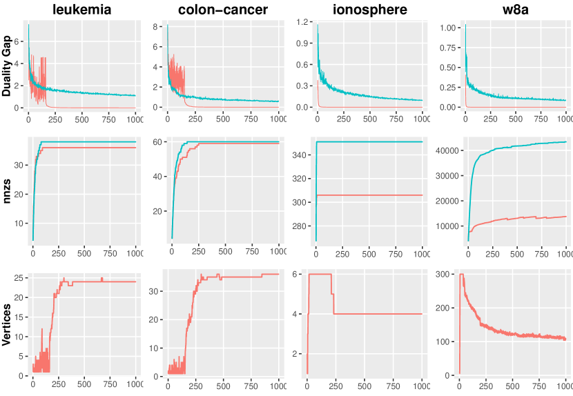
Figure 1: Convergence results for Alg. 1 (red) and randomized smoothing of Lan (2013) (blue) on the SVM datasets(51).

For this evaluation, we also compared our method with the randomized smoothing method of Lan (2013) shown in blue in Fig. 1. The top row of plots in Figure 1 ($y-$axis showing the duality gap) suggest that on all four datasets (leukemia, colon-cancer, ionosphere, w8a), the convergence of the baseline is slower as a function of the number of iterations. The second and the third row show that the coreset size and the vertices in $|V(Ax,\epsilon)|$ increase at most linearly with the number of iterations as predicted in Section (4.1.1). We see that the number of vertices in $|V(Ax,\epsilon)|$ remains very small throughout our experiments. While the convergence results shown for Lan (2013) are, in expectation, of the same order as the ones we show here, the bound is quite loose for these problems and we find that the practical convergence rate can be slow. This is especially important as the computation time of each iteration of that method increases with the iteration count, as more samples of the gradient are drawn in later iterations (unlike our algorithm). Moreover, Figure 2 shows that if we use a bisection line search instead of the step size policy suggested in the proof of Theorem 1, our algorithm actually converges (measured using the duality gap) in fewer than 40 iterations making it practically fast while also keeping our theoretical results intact.

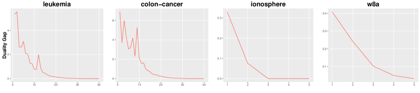
Figure 2: Convergence results for Alg. 1 using bisection line search.

5.2 The 1-median problem

We tested a simple Frank Wolfe based solver for the 1-median problem on synthetic data (similar to existing works for this problem). A set of points of size $n$ is sampled from a multivariate random Normal distribution. To keep the presentation succinct, we discuss those parts of this experiment that demonstrate additional useful properties of the algorithm beyond those described for $\ell_{1}$-SVM. The left plot in the top row of Figure 3 shows how the size of the coreset varies as we increase $n$ whereas the right plot shows the number of iterations required for convergence. Importantly, the size of the coreset is independent of $n$, as the problem we are solving is fundamentally no harder. The second row shows the computational time taken: left plot shows the total time taken whereas the right plot shows the time taken per iteration. We see that both of these scale sublinearly with the number of points. The plots agree with the theoretical results from earlier sections concerning the size of coreset and number of iterations required to obtain a solution.

5.3 Multiway Graph Cuts

In order to demonstrate that our algorithm is scalable to large datasets and hence it is practically applicable, we tested our algorithm on the dblife dataset Niu et al. (2011) which consists of 9168 labels. Therefore, $D$ is the product of $n$ 9168-dimensional simplices. Note that this problem consist of approximately 20 million decision variables and has been recently tackled via distributed schemes implemented on a cluster Niu et al. (2011). Due to the large of number of labels, this dataset is ideal for evaluating our algorithm as the analysis implies that the number of labels chosen must increase linearly with the number of iterations. This means that we get a sparse labeling scheme, i.e., the coreset here is the subset of the total number of labels. We evaluated this behavior by using increasing subsets of the total number of labels. We find that even when the total number of labels is small; this trend becomes more prominent as progressively larger sets of labels are used, shown in Figure 3 (row 3).

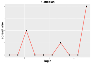
(a)

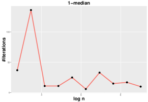
(b)

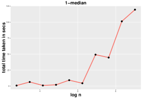
(c)

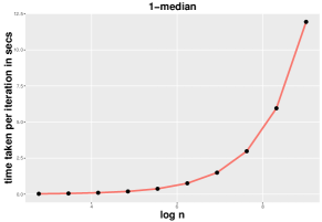
(d)

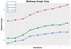
(e)

Figure 3: (Top row) Plotting the size of the coreset (left) and number of iterations (right) for 1-median as we vary the size $n$ of a randomly sampled set of points. We iterate until achieving a primal-dual gap of $10^{-6}$; $2^{\text{nd}}$ row shows the total time taken (left) and time taken per iteration (right); $3^{\text{rd}}$ row shows results for Graph cuts problem on dblife. Each LP subproblem took approximately 60 seconds using CPLEX solver.

Problem	$C_{f}$	Coreset
$\ell_{1}$-SVM	$\frac{2}{\epsilon}(\text{diam}_{\infty}(A^{+}\Delta_{m})+\text{diam}_{\infty}(A^{-}\Delta_{m}))$	Support vectors
1-median	$\frac{2}{\epsilon}\text{diam}_{2}(A\Delta_{n})^{2}$	Points
Graph cuts	$\frac{2}{\epsilon}(\text{diam}_{1}(AD))^{2}$	Labels
Balanced Development	$\frac{2}{\epsilon}(\text{diam}_{1}(A\Delta_{m}))^{2}$	Attributes
Sparse PCA with constraints	$\frac{2}{\epsilon}(\text{diam}_{\infty}(AS))^{2}$	Features

Table 1: A summary of the relevant quantities derived for each problem described in the previous sections.

5.4 Interesting empirical behavior and its potential relation to existing work

The experiments highlight two important practical aspects of the proposed algorithm.
A) How often do we encounter poor subproblems? The number of vertices in $|V(Ax,\epsilon)|$ given by our analysis seems to be an overestimate than what is practically observed. Assuming that we initialize at a point whose neighborhood does not contain any nonsmooth points, using the fact that the set of nondifferentiable points of a convex function on a compact set is of measure zero, we can show that the next iterate of the algorithm also does not contain any nonsmooth points in its neighborhood with high probability. But extending this argument to the next iterate becomes problematic. It seems like a Lovasz Local Lemma type result Kolmogorov (2015) will be able to shed some light on this behavior but the independence assumption is inapplicable, so one has to introduce randomness in the algorithm. But a separate sparsity analysis might have to be done to obtain coreset results.
B) Why does our algorithm converge so fast? The empirical behavior of certain algorithms have been strongly associated with the manifold identification property in recent works, see Lee and Wright (2012). Our algorithm when using a bisection line search strategy as shown in fig 3, converges within a few iterations and is faster than the state of the art solvers for that problem. It will be interesting to see if our algorithm satisfies some variation or extension of the properties that are described in Lee and Wright (2012), but one issue is that the algorithm presented in Lee and Wright (2012) has randomization incorporated at each iteration making it hard to adapt that analysis for our algorithm.
C) Tightness of convergence: Let us consider the case of $\ell_{1}$-SVM. Assume that the positive and negative labeled instances be generated by a Gaussian distribution with mean $0$ and $\mu$ respectively and variance $\sigma I$. Then we have that,

$$\mathbb{E}\left(\text{diam}_{\infty}(A^{+}\Delta_{m})+\text{diam}_{\infty}(A^{-}\Delta_{m})\right)\leq\sigma\log m+\mu+\sigma\log m=2\sigma\log m+\mu$$ (104)

using the properties of maximum of sub-gaussians. Here the expectation is taken over the randomness in the data: $A^{+},A^{-}$. This shows that the dependence of $C_{f}$ is logarithmic in the dimensions. Similarly we will get $\sqrt{n},n\log n$ for $\ell_{2},\ell_{1}$ norm diameters respectively showing that the $\mathbb{E}C_{f}$ is near linear in the dimensions. Now we plug this estimate in the convergence result in theorem (1),

$$\mathbb{E}\left(f(x_{k})-f(x_{*})\right)\leq\mathbb{E}\left(\frac{2^{5/2}L+2^{3/2}D_{f}}{\sqrt{k+2}}\right)=2^{5/2}\left(\frac{L+\mathbb{E}D_{f}}{\sqrt{k+2}}\right)=O\left(\frac{L+\log m}{\sqrt{k}}\right)$$ (105)

Hence we can see that by choosing an appropriate neighborhood depending on the application, we can get faster convergence. This aspect is either not present in other Frank Wolfe algorithms that solve nonsmooth problems or involve a looser dependence on the constants involved for example, Hazan and Kale (2012b) achieve a $O\left(\frac{Lm}{\sqrt{k}}\right)$ convergence compared to our $O\left(\frac{L+\log^{2}m}{\sqrt{k}}\right)$ here.

6 Discussion

We have presented novel coreset bounds and optimization schemes for nondifferentiable problems encountered in statistical machine learning and computer vision. The algorithm calculates sparse approximate solutions to the corresponding optimization problems deterministically in a number of iterations independent of the size of the input problem, depending only on the approximation factor and the sum of the Lipschitz constant and a nonlinearity term. The central result in Theorem 1 applies to any problem of the very general form in (1) with mild conditions, potentially suggesting a number of other applications beyond those considered here. Though a general condition to characterize all cases where the internal subproblem is efficiently solvable may not be available, we show a broad/useful class that is efficiently solvable.

Finally, we point out a few technical properties that differentiate our method from existing FW type methods for nonsmooth problems Argyriou et al. (2014); Pierucci et al. (2014).

First, many methods rely on smoothing the objective function by a prox function that needs to be designed piecemeal for specific problems. While examples exist where these functions can be readily derived, to our knowledge there are no standard recipes for deriving proximal functions in general. Second, several existing methods assume that the proximal iteration can be solved efficiently. However, it is known that in general, the worst case complexity of a single proximal iteration is the same as solving the original optimization problem Parikh and Boyd (2014). Third, it is not yet clear how coreset results can be derived for many existing methods, or if it is even possible. For example, (especially) in the very large scale setting, coreset results enable practical applications where one can store a subset of the (training) dataset and still be able to perform nearly as well (on the test data). The basic expectation is that more data should not always make a problem computationally harder. An exciting implication behind coreset results in (Clarkson, 2008) is that this can be avoided in certain cases. But (Clarkson, 2008) assumes that $f$ is smooth: an artifact of the optimization rather than a requirement of coresets per se — we showed that this assumption is not necessary at all. In closing, while the algorithm may not be the defacto off-the-shelf option for all nonsmooth problems, for many problems it offers a very competitive (generally applicable) alternative, and in certain cases, the theory nicely translates into significant practical benefits as well.

7 Acknowledgments

The authors are supported by NSF CAREER RI #1252725, NSF CCF #1320755, and UW CPCP (U54 AI117924). We thank Stephen J. Wright, Shuchi Chawla, Satyen Kale and Kenneth L. Clarkson for comments and suggestions.

References

- Acharya et al. [2015] J. Acharya, C. Daskalakis, and G. C. Kamath. Optimal testing for properties of distributions. In Advances in Neural Information Processing Systems, 2015.
- Agarwal et al. [2005] P. K. Agarwal, S. Har-Peled, and K. R. Varadarajan. Geometric approximation via coresets. Combinatorial and computational geometry, 2005.
- Argyriou et al. [2014] A. Argyriou, M. Signoretto, and J Suykens. Hybrid conditional gradient-smoothing algorithms with applications to sparse and low rank regularization. Regularization, Optimization, Kernels, and Support Vector Machines, 2014.
- Bach et al. [2012] F. Bach, R. Jenatton, J. Mairal, and G. Obozinski. Optimization with sparsity-inducing penalties. Foundations & Trends in Machine Learning, 2012.
- Balcan et al. [2013] M-F. Balcan, S. Ehrlich, and Y. Liang. Distributed -means and -median clustering on general topologies. In Advances in Neural Information Processing Systems, 2013.
- Banerjee et al. [2006] O. Banerjee, L.E. Ghaoui, A. d’Aspremont, and G. Natsoulis. Convex optimization techniques for fitting sparse gaussian graphical models. In Proceedings of the International Conference on Machine Learning (ICML), 2006.
- Bennett and Bredensteiner [2000] K. P. Bennett and E. J. Bredensteiner. Duality and geometry in SVM classifiers. In Proceedings of the International Conference on Machine Learning (ICML), 2000.
- Braverman and Chestnut [2014] V. Braverman and S. R. Chestnut. Streaming sums in sublinear space. CoRR, 2014.
- Clarkson [2008] K. L. Clarkson. Coresets, sparse greedy approximation, and the Frank-Wolfe algorithm. In Proceedings of the Symposium on Discrete Algorithms (SODA), 2008.
- Clarkson and Woodruff [2015] K. L. Clarkson and D. P. Woodruff. Input sparsity and hardness for robust subspace approximation. In Foundations of Computer Science, FOCS, 2015.
- Clarkson et al. [2012] K. L. Clarkson, E. Hazan, and D. P Woodruff. Sublinear optimization for machine learning. Journal of the ACM (JACM), 2012.
- Călinescu et al. [1998] G. Călinescu, H. Karloff, and Y. Rabani. An improved approximation algorithm for multiway cut. In Proceedings of the Symposium on Theory of Computing (STOC), 1998.
- Cui [2008] L. Cui. Maintenance models and optimization. In Handbook of performability engineering. 2008.
- Drineas et al. [2006] P. Drineas, R. Kannan, and M. W. Mahoney. Fast monte carlo algorithms for matrices i: Approximating matrix multiplication. SIAM Journal on Computing, 2006.
- Feldman et al. [2010] D. Feldman, M. Monemizadeh, C. Sohler, and D. P. Woodruff. Coresets and sketches for high dimensional subspace approximation problems. In Proceedings of the Symposium on Discrete Algorithms (SODA), 2010.
- Feldman et al. [2012] D. Feldman, A. Sugaya, and D. Rus. An effective coreset compression algorithm for large scale sensor networks. In Proceedings of the International Conference on Information Processing in Sensor Networks (IPSN), 2012.
- Frank and Wolfe [1956] M. Frank and P. Wolfe. An algorithm for quadratic programming. Naval Research Logistics Quarterly, 1956.
- Garber and Hazan [2011] D. Garber and E. Hazan. Approximating semidefinite programs in sublinear time. In Advances in Neural Information Processing Systems, 2011.
- Garber and Meshi [2016] D. Garber and O. Meshi. Linear-memory and Decomposition-invariant Linearly Convergent Conditional Gradient Algorithm for Structured Polytopes. ArXiv e-prints, 2016.
- Gärtner and Jaggi [2009] B. Gärtner and M. Jaggi. Coresets for polytope distance. In Proceedings of the ACM Symposium on Computation Geometry (SoCG), 2009.
- Gidel et al. [2017] G. Gidel, T. Jebara, and S. Lacoste-Julien. Frank-wolfe algorithms for saddle point problems. In Proceedings of the Artificial Intelligence and Statistics (AISTATS), 2017.
- Gilbert [19660] E. G. Gilbert. An iterative procedure for computing the minimum of a quadratic form on a convex set. SIAM Journal on Control, 19660.
- Grbovic et al. [2012] M. Grbovic, C. R. Dance, and S. Vucetic. Sparse principal component analysis with constraints. In Proceedings of the AAAI Conference on Artificial Intelligence, 2012.
- Günlük and Linderoth [2012] O. Günlük and J. Linderoth. Perspective reformulation and applications. In Mixed Integer Nonlinear Programming. 2012.
- Har-Peled and Kushal [2005] S. Har-Peled and A. Kushal. Smaller coresets for -median and -means clustering. In Proceedings of the ACM Symposium on Computation Geometry (SoCG), 2005.
- Har-Peled et al. [2007] S. Har-Peled, D. Roth, and D. Zimak. Maximum margin coresets for active and noise tolerant learning. In International joint conference on Artifical intelligence, 2007.
- Hazan and Kale [2012a] E. Hazan and S. Kale. Projection-free online learning. In Proceedings of the International Conference on Machine Learning (ICML), 2012a.
- Hazan and Kale [2012b] E. Hazan and S. Kale. Projection-free online learning. arXiv preprint arXiv:1206.4657, 2012b.
- Hiriart-Urruty and Lemaréchal [1993] J.-P. Hiriart-Urruty and C. Lemaréchal. Convex Analysis and Minimization Algorithms. Springer, 1993.
- Jaggi [2011] M. Jaggi. Sparse convex optimization methods for machine learning. PhD thesis, Eidgenössische Technische Hochschule ETH Zürich, Nr. 20013, 2011.
- Jaggi [2013] M. Jaggi. Revisiting Frank-Wolfe: Projection-free sparse convex optimization. In Proceedings of the International Conference on Machine Learning (ICML), 2013.
- Kolmogorov [2015] V. Kolmogorov. Commutativity in the random walk formulation of the lovasz local lemma. arXiv preprint arXiv:1506.08547, 2015.
- Lan [2013] G. Lan. The complexity of large-scale convex programming under a linear optimization oracle. arXiv preprint arXiv:1309.5550, 2013.
- Lee and Wright [2012] S. Lee and S. J. Wright. Manifold identification in dual averaging for regularized stochastic online learning. Journal of Machine Learning Research, 2012.
- Liu et al. [2009] H. Liu, M. Palatucci, and J. Zhang. Blockwise coordinate descent procedures for the multi-task lasso, with applications to neural semantic basis discovery. 2009.
- Mangasarian [1999] O. L. Mangasarian. Generalized support vector machines. Advances in Neural Information Processing Systems (NIPS), 1999.
- Nathan and Raghvendra [2014] V. Nathan and S. Raghvendra. Accurate Streaming Support Vector Machines. ArXiv e-prints, 2014.
- Nesterov [2005] Y. Nesterov. Smooth minimization of non-smooth functions. Mathematical programming, 2005.
- Nesterov [2009] Y. Nesterov. Primal-dual subgradient methods for convex problems. Technical report, 2009.
- Nesterov [2015] Y. Nesterov. Complexity bounds for primal-dual methods minimizing the model of objective function. Technical report, 2015.
- Niu et al. [2011] F. Niu, B. Recht, C. Ré, and S. J. Wright. Hogwild!: A lock-free approach to parallelizing stochastic gradient descent. In Neural Information Processing Systems, 2011.
- Parikh and Boyd [2014] N. Parikh and S. P. Boyd. Proximal algorithms. Foundations and Trends in Optimization, 2014.
- Pennanen [2012] T. Pennanen. Introduction to convex optimization in financial markets. Mathematical Programming, 2012.
- Pierucci et al. [2014] F. Pierucci, Z. Harchaoui, and J. Malick. A smoothing approach for composite conditional gradient with nonsmooth loss. PhD thesis, INRIA Grenoble, 2014.
- Robinson [2012] S. M. Robinson. Convexity in finite-dimensional spaces. Preprint, 2012.
- Rudelson and Vershynin [2007] M. Rudelson and R. Vershynin. Sampling from large matrices: An approach through geometric functional analysis. Journal of the ACM (JACM), 2007.
- Sarlos [2006] T. Sarlos. Improved approximation algorithms for large matrices via random projections. In Foundations of Computer Science (FOCS), 2006.
- Tsang et al. [2005] I. W. Tsang, J. T. Kwok, and P-M. Cheung. Core vector machines: Fast svm training on very large data sets. Journal of Machine Learning Research, 2005.
- White [1993] D. J. White. Extension of the Frank-Wolfe algorithm to concave nondifferentiable objective functions. Journal of Optimization Theory and Applications, 1993.
- Yuan et al. [2010] G.-X. Yuan, K.-W. Chang, C.-J. Hsieh, and C.-J. Lin. A comparison of optimization methods and software for large-scale L1-regularized linear classification. Journal of Machine Learning Research (JMLR), 2010.