Towards a Holistic Integration of Spreadsheets with Databases: A Scalable Storage Engine for Presentational Data Management
[Technical Report]

Abstract

Spreadsheet software is the tool of choice for interactive ad-hoc data management, with adoption by billions of users. However, spreadsheets are not scalable, unlike database systems. On the other hand, database systems, while highly scalable, do not support interactivity as a first-class primitive. We are developing DataSpread , to holistically integrate spreadsheets as a front-end interface with databases as a back-end datastore, providing scalability to spreadsheets, and interactivity to databases, an integration we term presentational data management (PDM). In this paper, we make the first step towards this vision: developing a storage engine for PDM, studying how to flexibly represent spreadsheet data within a database and how to support and maintain access by position. We first conduct an extensive survey of spreadsheet use to motivate our functional requirements for a storage engine for PDM. We develop a natural set of mechanisms for flexibly representing spreadsheet data and demonstrate that identifying the optimal representation is NP-Hard; however, we develop an efficient approach to identify the optimal representation from an important and intuitive subclass of representations. We extend our mechanisms with positional access mechanisms that don’t suffer from cascading update issues, leading to constant time access and modification performance. We evaluate these representations on a workload of typical spreadsheets and spreadsheet operations, providing up to 50% reduction in storage, and up to 50% reduction in formula evaluation time.

I Introduction

We are witnessing an increasing availability of data across a spectrum of domains, necessitating interactive ad-hoc management of this data: a business owner may want to manage customer data and invoices, a scientist experimental measurements, and a fitness enthusiast heart rate and activity traces. However, while there are two major software paradigms for supporting interactive ad-hoc data management—spreadsheets and databases—neither of them fulfill the desired requirements, as we illustrate using two real use-cases below:

Example 1 (Using Spreadsheets for Genomic Data Analysis).

During the course of genomic data analysis, biologists, such as our collaborators at the KnowEnG center at Mayo Clinic, generate data describing genomic variants as VCF (variant cell format) files, akin to CSV files. These VCF files are large, with tens of millions of rows and hundreds of columns, plus a raw size of many gigabytes. Unfortunately, many biologists, like scientists in many other domains, are adept at using spreadsheet software, but are not comfortable enough with programming to use databases. To interactively explore or browse their VCF data, they struggle to load such files into spreadsheet software: e.g., Microsoft Excel limits uploaded datasets to 1M rows and Google Sheets to 2M cells. And even when one can load large datasets, these tools become sluggish and unresponsive. In fact, many biologists are unable to explore the datasets they themselves create, instead sending them to bioinformatics collaborators to analyze.

Example 2 (Using Databases for Customer Management).

The owner of a small retail startup in Champaign, Illinois created a MySQL database for managing customers and sales, organized in a schema comprising 15 tables. There are several actions that he and his staff would like to routinely perform, such as insert (customers), modify (due dates of invoices), filter (overdue invoices), join (invoices and payments), and aggregate (the total amounts). To perform these operations without requiring SQL, he has to employ a programmer to develop database applications. Instead, he wants to interactively manipulate data for ad-hoc operations, but no such tools exist.

As these common use cases demonstrate, we are critically lacking a solution for interactive ad-hoc management of data. On the one hand, spreadsheet software, while being heralded as a prime example of a direct manipulation [34] tool, lacks scalability, due to its inability to operate on datasets that go beyond main memory capabilities, and expressiveness, since its formulae only operate on one cell at a time, necessitating complex means (e.g., VLOOKUP) to orchestrate simple operations like joins. On the other hand, while databases provide both scalability and expressiveness, they lack support for direct manipulation vital for interactive ad-hoc data management. Thus, users access databases either via pre-programmed database applications (Figure 1a), or SQL clients (Figure 1b), which only support operations on entire relations at a time, as opposed to directly interacting with data for ad-hoc updates and analysis. To this end, there has been a number of papers on making databases usable, e.g.,  [20, 28, 24, 19, 3], but this research has not witnessed widespread adoption.

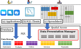
Figure 1: Connecting spreadsheets and databases for Presentational Data Management.

To address this, we are building a system, DataSpread, with spreadsheets as a front-end interface, and databases as a back-end datastore, with dual objectives: (i) allowing users to manipulate data from databases on a spreadsheet interface, without relying on pre-programmed applications or SQL clients—thereby enabling interactive ad-hoc data management for a database, while (ii) operating on datasets not limited by main memory—thereby addressing the key limitation of present-day spreadsheets. We call this new research direction of holistically integrating spreadsheets and databases presentational data management (PDM). In PDM, using a system like DataSpread, a user can view, analyze, and manipulate data in a presentational (i.e., spatial) interface (Figure 1c), in addition to standard approaches (Figure 1a,b). They can import large tables (e.g., VCF files) from/to the interface or database, and arrange them on the interface. They can also operate at various granularities, embodying the principles of direct manipulation [34]—from cells (like a spreadsheet) to tables (like a database)—adding computation in the form of formulae or queries as part of the interface, in addition to data. This can result in various forms of arrangement of data, ranging from structured tables, reports, and forms, to ad-hoc presentations of data embedded with computation. They can also refer to data by tables or attributes (as in a database) or position (as in a spreadsheet). While we primarily focus on spreadsheets, similar considerations apply for other presentational interfaces for interactive ad-hoc data management.

While developing DataSpread is a multi-year vision, we have already made significant headway, with a functional prototype (see http://dataspread.github.io). In this paper, we focus on the following fundamental question—how do we develop a storage manager to support presentational data management (PDM)?

Requirements for a PDM Storage Engine. In developing a storage engine for PDM, we conduct a survey and user study (Section II) to characterize two key functional requirements for such a storage engine to support the direct manipulation of data in a presentational interface (such as a spreadsheet):

(i) Presentational Awareness. A storage engine for PDM must be aware of the layout of data within the spreadsheet interface and be flexible enough to adapt to various ad-hoc modalities users might choose to lay out and manage data (and queries) on spreadsheets, ranging from fully structured tables, to data scattered across the spreadsheet, along with formulae.

(ii) Presentational Access. A storage engine for PDM must support access of a range of data by position: for example, users may scroll to a certain region of the spreadsheet, or a formula may access a range of cells; this access must be supported as a first-class primitive.

Challenges in Supporting PDM. In supporting these functional requirements, our first set of challenges emerge in how we can flexibly represent presentational information within a database. A user may manage several table-like regions within a spreadsheet, interspersed with empty rows or columns, along with formulae. One option is to store the spreadsheet as a single relation, with tuples as spreadsheet rows, and attributes as spreadsheet columns—this can be very wasteful due to sparsity. Another option is to store the filled-in cells as key-value pairs: [(row #, column #), value]; this can be effective for sparse spreadsheets, but is wasteful for dense spreadsheets with well-defined tables. One can imagine hybrid representation schemes using both “dense” and “sparse” schemes, as well as those that take access patterns, e.g., via formulae, into account. Unfortunately, we show that it is NP-Hard to identify the optimal representation.

Our second set of challenges emerge in supporting and maintaining presentational access. Say we use a single relation to record information about a sheet, with one tuple for each spreadsheet row, and one attribute for each spreadsheet column; with an additional attribute that records the spreadsheet row number. Now, inserting a single row in the spreadsheet can lead to an expensive cascading update of the row numbers of all subsequent rows; thus, we must develop techniques that allow us to avoid this issue. Moreover, we need positional indexes that can access a range of rows at a time, say, when a user scrolls to a certain region of the spreadsheet. While one could use a traditional index (e.g., a B+ tree) on the attribute corresponding to row number, the cascading update makes it hard to maintain such an index across edit operations.

Our Contributions. In this paper, we address the aforementioned challenges in developing a scalable storage manager for PDM. Our contributions are the following:

1. Understanding Present-day Solutions for PDM

. We perform an empirical study of four spreadsheet datasets plus a user survey to understand how spreadsheets are presently used for data manipulation and analysis (Section II).

2. Abstracting the Functional Requirements

. Based on our study, we define our conceptual data model, as well as the operations necessary for PDM (Section III).

3. Primitive Representation Schemes for PDM

. We propose four primitive data models that implement the conceptual data model, and demonstrate that they represent “optimal extreme choices” (Section IV-B).

4. Near-Optimal Hybrid Representation Schemes for PDM

. We develop a space of hybrid data models, utilizing these primitive data models, and demonstrate that identifying the optimal hybrid is NP-Hard (Section IV-C); we further develop multiple PTIME solutions that provide near-optimality (Section IV-D), plus greedy heuristics (Section IV-E), and show that they can be incrementally maintained (Section IV-F).

5. Presentational Access Schemes for PDM

. We develop solutions to maintain positional information, while reducing the impact of cascading updates (Section V).

6. Prototype of DataSpread

. We have developed a fully functional prototype of DataSpread, and describe its functionalities that go beyond the storage manager (Section VI).

7. Experimental Evaluation

. We evaluate our data models and presentational access schemes on a variety of real-world and synthetic datasets, demonstrating that our storage engine is scalable and efficient (Section VII). We also conduct a small qualitative evaluation to illustrate how DataSpread can handle the use-cases described earlier.

Related Work. While there have been attempts at combining spreadsheets and relational database functionality, ultimately, all of these attempts fall short because they do not let spreadsheet users perform ad-hoc data manipulation operations [46, 47, 26]; there have also been efforts that enhance spreadsheets or databases without combining them e.g., [37]. We describe this and other related work in detail in Section VIII.

Dataset	Sheets	Formulae Distribution			Density Distribution		Tabular Regions		Formula Access
		Sheets with	Sheets with	%formulae	Sheets with	Sheets with	Tables	%Coverage	Cells Accessed	Tabular Regions
		formulae	$>20\%$ formulae	coverage	$<50\%$ density	$<20\%$ density			per formula	per formula
Internet	52,311	29.15%	20.26%	1.30%	22.53%	6.21%	67,374	66.03%	334.26	2.50
ClueWeb09	26,148	42.21%	27.13%	2.89%	46.71%	23.8%	37,164	67.68%	147.99	1.92
Enron	17,765	39.72%	30.42%	3.35%	50.06%	24.76%	9,733	60.98%	143.05	1.75
Academic	636	91.35%	71.26%	23.26%	90.72%	60.53%	286	12.10%	3.03	1.54

TABLE I: Spreadsheet Datasets: Preliminary Statistics.

(a)

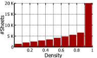
(b)

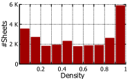
(c)

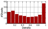
(d)

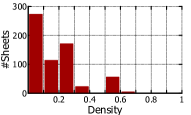
Figure 2: Data Density — (a) Internet. (b) ClueWeb09. (c) Enron. (d) Academic.

(a)

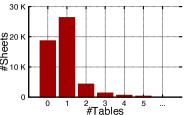
(b)

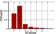
(c)

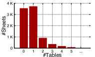
(d)

Figure 3: Tabular Region Distribution - (a) Internet. (b) ClueWeb09. (c) Enron. (d) Academic.

(a)

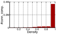
(b)

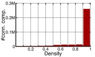
(c)

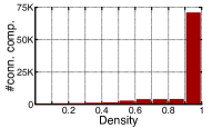
(d)

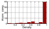
Figure 4: Connected Component Data Density — (a) Internet. (b) ClueWeb09. (c) Enron. (d) Academic.

(a)

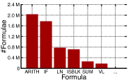
(b)

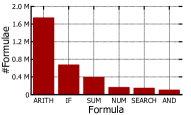
(c)

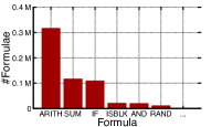
(d)

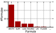
Figure 5: Formulae Distribution — (a) Internet. (b) ClueWeb09. (c) Enron. (d) Academic.

II Understanding Current Solutions for PDM

We now perform an empirical study to characterize the functional requirements for a storage engine for PDM. We hypothesize that understanding the present-day use of spreadsheets for managing data is a suitable proxy for understanding the requirements of PDM; of course, since current spreadsheets are limited to those that can be manipulated in current software, they are smaller than what we aim to support in DataSpread.

We focus on two aspects: (i) identifying how users structure data on the interface, and (ii) understanding common interface operations. To do so, we first retrieve spreadsheets from four sources and quantitatively analyze them on different metrics. We supplement this analysis with a small-scale user survey to understand the spectrum of operations frequently performed. The latter is necessary since we do not have a readily available trace of user operations (e.g., how often do users add rows).

We first describe our methodology for both these evaluations, before diving into our findings.

II-A Methodology

As described above, we have two forms of evaluation.

II-A1 Real Spreadsheet Datasets

For our evaluation of real spreadsheets, we assemble the following four datasets from a wide variety of sources.

Internet. This dataset of 53k spreadsheets was generated by using Bing to search for .xls files, using a variety of keywords. As a result, these 53k spreadsheets vary widely in content, ranging from tabular data to images.

ClueWeb09. This dataset of 26k spreadsheets was generated by extracting .xls file URLs from the ClueWeb09 [10] crawl.

Enron. This dataset was generated by extracting 18k spreadsheets from the Enron email dataset [23]. These spreadsheets were used to exchange data within the Enron corporation.

Academic. This dataset was collected from an academic institution using spreadsheets to manage administrative data.

We list these four datasets in Table I. The first two datasets are primarily meant for data publication: thus, only about 29% and 42% of these sheets (column 3) contain formulae, with the formulae occupying less than 3% of the total number of non-empty cells for both datasets (column 5). The third dataset is primarily meant for email-based data exchange, with a similarly low fraction of 39% of these sheets containing formulae, and 3.35% of the non-empty cells containing formulae. The fourth dataset is primarily meant for data analysis, with a high fraction of 91% of the sheets containing formulae, and 23.26% of the non-empty cells containing formulae.

II-A2 User Survey

To evaluate the kinds of operations performed on spreadsheets, we solicited 30 participants from industry who exclusively used spreadsheets for data management, for a qualitative user survey. This survey was conducted via an online form, with the participants answering a small number of multiple-choice and free-form questions, followed by the authors aggregating the responses.

II-B Structure Evaluation

We begin by asking: how do users structure data in PDM? Is the data typically organized and structured into tables, or is it largely unstructured? Does the type of structure depend on the intended use-case?

Across Spreadsheets: Data Density. To evaluate whether real spreadsheets are similar to structured relational data, we first we estimate the density of each sheet, defined as the ratio of the number of filled-in cells to the number of cells within the minimum bounding rectangular box enclosing the filled-in cells. We depict the results in the last two columns of Table I: the spreadsheets in Internet, Clueweb09, and Enron are typically dense, i.e., more than $50\%$ of the spreadsheets have density greater than $0.5$. On the other hand, for Academic, a high proportion (greater than $60\%$) of the spreadsheets have density values less than $0.2$. This low density is because the latter dataset embeds many formulae and uses forms to report data in a user-accessible interface.

Takeaway 1 (Presentational Awareness): Structure in PDM can vary widely, from highly sparse to highly dense, necessitating data models that can adapt to such variations.

Within a Spreadsheet: Tabular regions. We further analyzed the sparse spreadsheets to evaluate whether there are regions within them with high density—essentially indicating that these are structured tabular regions. To do so, we first constructed a graph of the filled-in cells within each spreadsheet, where two cells (i.e., nodes) have an edge between them if they are adjacent. We then computed the connected components of this graph. We declare a connected component to be a tabular region if it spans at least two columns and five rows, and has a density of at least $0.7$, defined as before. In Table I, for each dataset, we list the total number of identified tabular regions (column 8) and the fraction of the total filled-in cells that are captured within these tabular regions (column 9). In Figure 3 we plot the distribution of tables across our datasets. For Internet, ClueWeb09, and Enron, we observe that greater than $60\%$ of the cells are part of tabular regions. For Academic, where the sheets are rather sparse, there still are a modest number of regions that are tabular (286 across 636 sheets).

We next characterize the connected components by understanding how they conform to a tabular structure. To study this, we estimate the density of each connected component, defined as the ratio of the number of filled-in cells to the number of cells within the minimum bounding rectangular box enclosing the connected component. Figure 4 depicts the density distribution of connected components. We note that across all the four data sets the connected components are very dense, specifically more than $80\%$ of the spreadsheets have density greater than $0.8$.

Takeaway 2 (Presentational Awareness): Even within a single spreadsheet, there is often high skew, with areas of high and low density, indicating the need for fine-grained data models that can treat these regions differently.

II-C Operation Evaluation

We now ask: What kinds of operations do users naturally perform in PDM? How often do users employ data manipulation operations? Or analysis operations, e.g., formulae? How do users refer to the portions of data in the operations?

Popularity: Formulae Usage. Formulae use is common, but there is a high variance in the fraction of cells that are formulae (see column 5 in Table I), ranging from 1.3% to 23.26%. We note that Academic embeds a high fraction of formulae since their spreadsheets are used primarily for data management as opposed to sharing or publication. Despite that, all of the datasets have a substantial fraction of spreadsheets where the formulae occupy more than 20% of the cells (column 4)—20.26% and higher for all datasets.

Takeaway 3 (Presentational Access): Formulae are very common, with over 20% of the spreadsheets containing a significant fraction of over $\frac{1}{5}$ of formulae. Optimizing for the access patterns of formulae when developing data models is crucial.

Formulae Distribution and Patterns. Next, we study the distribution of formulae used within spreadsheets—see Figure 5. Not surprisingly, arithmetic operations (ARITH, LN, SUM) are very common, along with conditional formulae (IF, ISBLK). Overall, there is a wide variety of formulae that span both a small number of cell accesses (e.g., arithmetic), as well as a large number of them (e.g., SUM, VL short for VLOOKUP). Moreover, these formulae typically access a small number of rectangular region, i.e., an area defined by a set of contiguous rows and columns, at a time (column 11). Many of the formulae used ended up reproducing relational operations (e.g., VLOOKUP for joins).

To gain a better understanding of how much effort is necessary to execute these formulae, we measure the number of cells accessed by each formula. Then, we tabulate the average number of cells accesses per formula in column 10 of Table I for each dataset. As we can see in the table, the average number of cells accesses per formula is not small—with up to 300+ cells per formula for Internet, and about 140+ cells per formula for Enron and ClueWeb09. Academic has a smaller average number—many of these formulae correspond to derived columns that access a small number of cells at a time. Next, we check if the accesses made by these formulae were spread across the spreadsheet, or could exploit spatial locality. To measure this, we considered the set of cells accessed by each formula, and then generated the corresponding graph of these accessed cells as described in the previous subsection for computing the number of tabular regions. We then counted the number of connected components, shown in column $11$. Even though the number of cells accessed may be large, these cells stem from a small number of connected components; as a result, we can exploit spatial locality to execute them more efficiently.

Takeaway 4 (Presentational Access and Awareness): Formulae on spreadsheets access cells on the spreadsheet by position; some common formulae such as SUM or VLOOKUP access a rectangular range of cells at a time. The number of cells accessed by these formulae can be quite large, and most of these cells stem from contiguous areas of the spreadsheet.

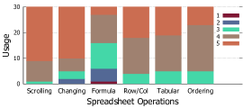
Figure 6: Operations performed on spreadsheets.

User-Identified Operations. We now analyze the common spreadsheet operations performed by users via a small-scale online survey of $30$ participants. This qualitative study is valuable since real spreadsheets do not reveal traces of user operations. Our questions in this study were targeted at understanding (i) how users perform operations on spreadsheets and (ii) how users organize data on spreadsheets.

We asked each participant to answer a series of questions where each question corresponded to whether they conducted the specific operation under consideration on a scale of 1–5, where 1 corresponds to “never” and 5 to “frequently”. For each operation, we plotted the results in a stacked bar chart in Figure 6, with the higher numbers stacked on the smaller ones.

We find that all the thirty participants perform scrolling, i.e., moving up and down the spreadsheet to examine the data, with 22 of them marking 5 (column 1). All participants reported to have performed editing of individual cells (column 2), and many of them reported to have performed formula evaluation frequently (column 3). Only four of the participants marked $<4$ for some form of row/column-level operations, i.e., deleting or adding one or more rows or columns at a time (column 4).

Takeaway 5 (Presentational Access and Awareness): There are several common operations performed by spreadsheet users including scrolling, row and column modification, and editing individual cells.

Our second goal for performing the study was to understand how users organize their data. We asked each participant if their data is organized in well-structured tables, or if the data scattered throughout the spreadsheet, on a scale of 1 (not organized)–5 (highly organized)—see Figure 6. Only five participants marked $<4$ which indicates that users do organize their data on a spreadsheet (column 5). We also asked the importance of ordering of records in the spreadsheet on a scale of 1 (not important)–5 (highly important). Unsurprisingly, only five participants marked $<4$ for this question (column 6). We also provided a free-form textual input where multiple participants mentioned that ordering comes naturally to them and is often taken for granted while using spreadsheets.

Takeaway 6 (Presentational Awareness): Spreadsheet users typically try to organize their data as far as possible on the spreadsheet, and rely heavily on the ordering and presentation of the data on their spreadsheets.

III Data Presentation Manager

Given our findings on presentational awareness and access, we now abstract out the functional requirements of the data presentation manager, the storage engine for PDM. We abstract out the presentational interface of a spreadsheet, as a conceptual data model, as well as the operations supported on it; concrete implementations will be described in subsequent sections. We will then describe our DataSpread prototype to place these requirements in context.

Conceptual Data Model. A spreadsheet consists of a collection of cells, referenced by two dimensions: row and column. Columns are referenced using letters A, $\ldots$, Z, AA, $\ldots$; while rows are referenced using numbers 1, $\ldots$ Each cell contains a value, or formula. A value is a constant; e.g., in Figure 7 (a DataSpread screenshot), B2 (column B, row 2) contains the value 10. In contrast, a formula is a mathematical expression that contains values and/or cell references as arguments, to be manipulated by operators or functions. For example, in Figure 7, cell F2 contains the formula =AVERAGE(B2:C2)+D2+E2, which unrolls into the value 85. In addition to a value or a formula, a cell could also additionally have formatting associated with it; e.g., width, or font. For simplicity, we ignore formatting aspects, but these aspects can be easily captured without significant changes.

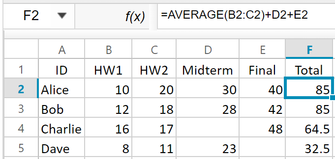
Figure 7: Sample Spreadsheet (DataSpread screenshot).

Spreadsheet-Oriented Operations. We now describe the spreadsheet-like operations necessary for PDM, drawing from our survey (takeaway 3-5).

1. Retrieving a Range. Our most basic read-only operation is getCells(range), where we retrieve a rectangular range of cells. This operation is relevant in scrolling, where the user moves to a specific position and we need to retrieve the rectangular range of cells visible at that position, e.g., range A1:F5, is visible in Figure 7. Similarly, formula evaluation also accesses one or more ranges of cells.

2. Updating an existing cell: The operation updateCell(row, column, value) corresponds to modifying the value of a cell.

3. Inserting/Deleting row/column(s): This operation corresponds to inserting/deleting row/column(s) at a specific position, followed by shifting subsequent row/column(s) appropriately: (i) insertRowAfter(row) (ii) insertColumnAfter(column) (iii) deleteRow(row) (iv) deleteColumn(column).

Database-Oriented Operations. We now describe the database-like operations for PDM, enabling users to effectively use the interface to manage and interact with database tables.

1. Link an existing table/Create a new table: This operation enables users to link a region on a spreadsheet with an existing database relation, establishing a two way correspondence between the spreadsheet interface and the underlying table, such that any operations on the spreadsheet interface are translated by the data presentation manager into table operations on the linked table. Thus, a user can use traditional spreadsheet operations such as updating a cell’s value to update a database table. We introduce the function: linkTable(range, tableName). If tableName does not exist, it will be created in the database, and then linked to the spreadsheet interface.

2. Relational Operators: Users can interact with the linked tables as well as other tabular regions via relational operators, as well as SQL, using the following spreadsheet functions: union, difference, intersection, crossproduct, join, filter, project, rename, and sql. These functions return a single composite table value; to retrieve the individual rows and columns within that table value, we have an index(cell, i, j) function that looks up the (i, j)th row and column in the composite table value in location cell, and places it in the current location.

Given the functional requirements for our data presentation manager, in Section IV, we develop concrete mechanisms for representing our conceptual data model in a database back-end, and in Section V, we develop data structures that enable efficient access in the presence of updates.

IV Presentational Awareness

We now describe the high-level problem of representation of spreadsheet data within a database; we will concretize this problem later. We focus on one spreadsheet, but our techniques seamlessly carry over to the multiple spreadsheet case.

RowID	$Col_{1}$	…	$Col_{6}$
1	ID, NULL	…	Total, NULL
2	Alice, NULL	…	85, AVERAGE(B2:C2)+D2+E2
…	…	…	…

ColID	$Row_{1}$	…	$Row_{5}$
1	ID,NULL	…	Dave,NULL
2	HW1,NULL	…	8,NULL
…	…	…	…

RowID	ColID	Value
1	1	ID, NULL
…	…	…, …
2	6	85, AVERAGE(B2:C2)+D2+E2
…	…	…, …

Figure 8: (a) Row-Oriented Model (b) Column-Oriented Model (c) Row-Column-Value Model for Figure 7.

IV-A High-level Problem Description

The conceptual data model corresponds to a collection of cells, represented as $C=\{C_{1},C_{2},\ldots,C_{m}\}$; as described previously, each cell $C_{i}$ corresponds to a location (i.e., a specific row and column), and has some contents—either a value or a formula. Our goal is to represent and store $C$, via one of the physical data models, $\mathds{P}$. Each $T\in\mathds{P}$ corresponds to a collection of relational tables $\left\{T_{1},\ldots,T_{p}\right\}$. Each table $T_{i}$ records the data in a certain portion of the spreadsheet. Given $C$, a physical data model $T$ is said to be recoverable with respect to $C$ if for each $C_{i}\in C,\exists$ precisely one $T_{j}\in T$ such that $T_{j}$ records the data in $C_{i}$. Our goal is to identify physical data models that are recoverable.

At the same time, we want to minimize the amount of storage required to record $T$, i.e., we would like to minimize $\operatorname{size}(T)=\sum_{i=1}^{p}\operatorname{size}(T_{i})$. Moreover, we would like to minimize the time taken for accessing data using $T$, i.e., the access cost, which is the cost of accessing a rectangular range of cells for formulae (takeaway 4) or scrolling (takeaway 5), both common operations. And we would like to minimize the time taken to perform updates, i.e., the update cost, which is the cost of updating cells, and the insertion and deletion of rows and columns.

Given a collection of cells $C$, our goal is to identify a physical data model $T$ such that: (i) $T$is recoverable with respect to $C$, and (ii) $T$minimizes a combination of storage, access, and update costs, among all $T\in\mathds{P}$.

We begin by considering the setting where the physical data model $T$ has a single relational table, i.e., $T=\left\{T_{1}\right\}$. We develop three ways of representing this table—we call them primitive data models—drawn from prior work, each of which works well for a specific structure of spreadsheet (Section IV-B). Then, we extend this to the setting where $|T|>1$ by defining hybrid data models with multiple tables each of which uses one of the three primitive data models to represent a certain portion of the spreadsheet (Section IV-C). Given the high diversity of structure within spreadsheets and high skew (takeaway 2), having multiple primitive data models, and the ability to use multiple tables, gives us substantial presentational awareness.

IV-B Primitive Data Models

Our primitive data models represent trivial solutions for spreadsheet representation with a single table. Before we describe these data models, we discuss a small wrinkle that affects all of these models. To capture a cell’s position we need to record a row and column number with each cell. Say we use an attribute to capture the row number for a cell. Then, any insertion or deletion of rows requires cascading updates to the row number attribute for cells in all subsequent rows. As it turns out, all of the data models we describe here suffer from performance issues arising from cascading updates, but the solution to deal with this issue is similar for all of them, and will be described in Section V. Thus, we focus here on storage and access cost. Also, note that the access and update cost of data models depends on whether the underlying database is a row or a columnar store. We use a row store, which our DataSpread implementation employs, and is suitable for a hybrid read-write setting. We now describe the primitive data models:

Row-Oriented Model (ROM). The row-oriented data model is akin to the traditional relational data model. We represent each row from the sheet as a separate tuple, with an attribute for each column $Col1$, $\ldots$, $Colc_{max}$, where $Colc_{max}$ is the largest non-empty column, and an additional attribute for explicitly capturing the row number, i.e., $RowID$. The schema for ROM is: ROM($RowID$, $Col1$, $\ldots$, $Colc_{max}$)—we illustrate the ROM representation of Figure 7 in Figure 8(a): each entry is a pair corresponding to a value and a formula, if any. For dense spreadsheets that are tabular (takeaways 1 and 2), this data model can be quite efficient in storage and access, since each row number is recorded only once, independent of the number of columns. Overall, ROM shines when entire rows are accessed at a time. It is also efficient for accessing a large range of cells at a time.

Column-Oriented Model (COM). The second representation is the transpose of ROM. Often, we find that certain spreadsheets have many columns and relatively few rows, necessitating such a representation. The schema for COM is: COM($ColID$, $Row1$, $\ldots$, $Rowr_{max}$). Figure 8(b) illustrates the COM representation of Figure 7. Like ROM, COM shines for dense data; while ROM shines for row-oriented operations, COM shines for column-oriented operations.

Row-Column-Value Model (RCV). The Row-Column-Value Model is inspired by key-value stores, where the Row-Column number pair is treated as the key. The schema for RCV is RCV($RowID$, $ColID$, $Value$). The RCV representation for Figure 7 is provided in Figure 8(c). For sparse spreadsheets often found in practice (takeaway 1 and 2), this model is quite efficient in storage and access since it records only the filled in cells, but for dense spreadsheets, it incurs the additional cost of recording and retrieving the row and column numbers for each cell as compared to ROM and COM, and has a much larger number of tuples. RCV is also efficient when it comes to retrieving specific cells at a time.

Why these Data Models? Readers may be wondering why we chose these data models (ROM, COM and RCV). As it turns out, these data models represent extremes in a space of data models that we identify and refer to as rectangular data models. We can further demonstrate that these three models do not dominate each other, i.e., there are settings where each of them prevails and are optimal within the space of rectangular data models. We refer the reader to Appendix D for details.

Database-Linked Tables. Such tables are not represented using primitive data models, instead stored as-is in the database. We refer to this as a Table-Oriented Model (TOM). Our linkTable operation sets up a two-way synchronization between a database table and a spreadsheet table.

IV-C Hybrid Data Model: Intractability

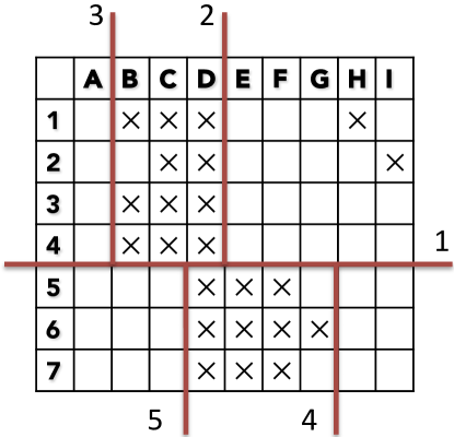
Figure 9: Hybrid Data Model: Recursive Decomposition.

So far, we developed the primitive data models to represent a spreadsheet using a single table in a database. We now develop better solutions by decomposing a spreadsheet into multiple regions, each represented by one of the primitive data models. We call these hybrid data models.

Definition 1 (Hybrid Data Models).

Given a collection of cells $C$, we define hybrid data models as the space of physical data models that are formed using a collection of tables $T$ such that $T$ is recoverable with respect to $C$, and further, each $T_{i}\in T$ is either a ROM, COM, RCV, or a TOM table.

As an example, for the spreadsheet in Figure 9, we might want the dense areas, i.e., B1:D4 and D5:G7, represented via a ROM table each and the remaining area, specifically, H1 and I2 to be represented by an RCV table.

Cost Model. As discussed earlier, the storage, access, and update costs impact our choice of data model. For this section, we focus exclusively on storage. We will generalize to access cost in Appendix A-C. The update cost will be the focus of the next section. Furthermore, we begin with ROM; we will generalize to RCV and COM in Section IV-F.

Given a hybrid data model $T=\left\{T_{1},\ldots,T_{p}\right\}$, where each ROM table $T_{i}$ has $r_{i}$ rows and $c_{i}$ columns, the cost of $T$ is

$$\operatorname{cost}(T)= \sum_{i=1}^{p}s_{1}+s_{2}\cdot(r_{i}\times c_{i})+s_{3}\cdot c_{i}+s_{4}\cdot r_{i}.\vspace{-5pt}$$ (1)

Here, the constant $s_{1}$ is the cost of initializing a new table, while the constant $s_{2}$ is the cost of storing each individual cell (empty or not) in the ROM table. The non-empty cells that have content may require additional storage; however, this is a constant cost that does not depend on the data model. The constant $s_{3}$ is the cost corresponding to each column, while $s_{4}$ is the cost corresponding to each row. The former is necessary to record schema information per column, while the latter is necessary to record the row information in the $RowID$ attribute. Overall, while the specific costs $s_{i}$ may differ across databases, what is clear is that all of these costs matter.

Formal Problem. We now state our formal problem below.

Problem 1 (Hybrid-ROM).

Given a spreadsheet with a collection of cells $C$, identify the hybrid data model $T$ with only ROM tables that minimizes $\operatorname{cost}(T)$.

Unfortunately, Problem 1 is NP-Hard, via a reduction from the minimum edge length partitioning of rectilinear polygons problem [25] of finding a partitioning of a polygon whose edges are aligned to the X and Y axes, into rectangles, while minimizing the total perimeter; see Appendix A-A.

Theorem 1 (Intractability).

Problem 1 is NP-Hard.

IV-D Optimal Recursive Decomposition

Instead of directly solving Problem 1, which is intractable, we instead aim to make it tractable, by reducing the search space of solutions. In particular, we focus on hybrid data models that can be obtained by recursive decomposition. Recursive decomposition is a process where we repeatedly subdivide the spreadsheet area from $[1\ldots r_{max},1\ldots c_{max}]$ by using a vertical cut between two columns or a horizontal cut between two rows, and then recurse on the resulting areas. As an example, in Figure 9, we can make a cut along line 1 horizontally, giving us two regions from rows 1 to 4 and rows 5 to 6. We can then cut the top portion along line 2 vertically, followed by line 3, separating out one table B1:D4. By cutting the bottom portion along line 4 and line 5, we can separate out the table D5:G7. Further cuts can help us carve out tables out of H1 or I2, not depicted here.

As the example illustrates, recursive decomposition is very powerful, since it captures a broad space of hybrid models; basically, anything that can be obtained via recursive cuts along the $x$ and $y$ axis. Unfortunately, there is an exponential number of such models. Now, a natural question is: what sorts of hybrid data models cannot be composed via recursive decomposition?

Observation 1 (Counterexample).

In Figure 10(a), the tables: A1:B4, D1:I2, A6:F7, and H4:I7 cannot be obtained via recursive decomposition.

To see this, note that any vertical or horizontal cut that one would make at the start would cut through one of the four tables, making the decomposition impossible. Nevertheless, we expect this form of construction to not be frequent, whereby the hybrid data models obtained via recursive decomposition form a natural class of data models.

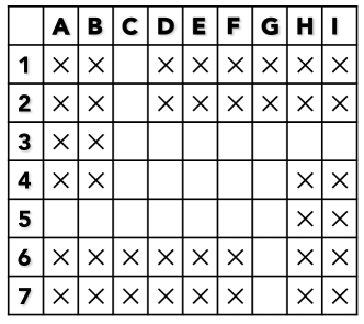
Figure 10: (a) Counterexample. (b) Weighted Representation.

Despite the space of recursively decomposed hybrid data models being exponential, as it turns out, identifying the optimal data model in this space to Problem 1 is PTIME. We use dynamic programming; our algorithm makes the most optimal “cut” horizontally or vertically at every step, and proceeds recursively; details below.

Consider a rectangular area formed from $x_{1}$ to $x_{2}$ as the top and bottom row numbers respectively, both inclusive, and from $y_{1}$ to $y_{2}$ as the left and right column numbers respectively, both inclusive, for some $x_{1},x_{2},y_{1},y_{2}$. Now, the optimal cost of representing this rectangular area, i.e., $\operatorname{Opt}((x_{1},y_{1}),(x_{2},y_{2}))$, is the minimum of the following possibilities:

• If there is no filled cell in the area $(x_{1},y_{1}),(x_{2},y_{2})$, then we do not use any data model, and the cost is $0$.

• Do not split, i.e., store as a ROM model ($\operatorname{romCost}()$):

  $$\operatorname{romCost}((x_{1},y_{1}),(x_{2},y_{2}))=s_{1}+s_{2}\cdot(r_{12}\times c_{12})\\ +s_{3}\cdot c_{12}+s_{4}\cdot r_{12},$$ (2)

  where number of rows $r_{12}=(x_{2}-x_{1}+1)$, and the number of columns $c_{12}=(y_{2}-y_{1}+1)$.

• Perform a horizontal cut ($C_{H}$):

  $$C_{H}=\min_{i\in\{x_{1},\ldots,x_{2}\}}\!\!\!\!\!\operatorname{Opt}((x_{1},y_{1}),(i,y_{2}))\\ +\operatorname{Opt}((i+1,y_{1}),(x_{2},y_{2}))$$ (3)

• Perform a vertical cut ($C_{V}$):

  $$C_{V}=\min_{j\in\{y_{1},\ldots,y_{2}\}}\!\!\!\!\!\operatorname{Opt}((x_{1},y_{1}),(x_{2},j))\\ +\operatorname{Opt}((x_{1},j+1),(x_{2},y_{2}))$$ (4)

Therefore, when there are filled cells in the rectangle,

$$\operatorname{Opt}((x_{1},y_{1}),(x_{2},y_{2}))=\\ \min\big{(}\operatorname{romCost}(\left(x_{1},y_{1}\right),\left(x_{2},y_{2}\right)),C_{H},C_{V}\big{)}.$$

The base case is when the rectangular area is of dimension $1\times 1$. Here, we store the area as a ROM table if it is filled. Hence, we have, $\operatorname{Opt}((x_{1},y_{1}),(x_{1},y_{1}))=c_{1}+c_{2}+c_{3}+c_{4}$, if filled, and $0$ if not.

We have the following theorem:

Theorem 2 (Dynamic Programming Optimality).

For the exponential space of ROM-based hybrid data models based on recursive decomposition, we can obtain the optimal solution via dynamic programming in PTIME.

Time Complexity. Our dynamic programming algorithm runs in polynomial time with respect to the size of the spreadsheet. Let the length of the larger side of the minimum enclosing rectangle of the spreadsheet be of size $n$. Then, the number of candidate rectangles is $\mathcal{O}(n^{4})$. For each rectangle, we have $\mathcal{O}(n)$ ways to perform the cut. Therefore, the running time of our algorithm is $\mathcal{O}(n^{5})$. However, this number could be very large if the spreadsheet is massive–which is typical of the use-cases we aim to tackle.

Approximation Bound. Even though our dynamic programming algorithm only identifies the best recursive decomposition based hybrid data model, we can derive a bound for its cost relative to the best hybrid data model overall. We refer the reader to Appendix A-B for the proof.

Theorem 3 (Approximation Bound ).

Say there are $k$ rectangles in the optimal decomposition with cost $c$. Then, the recursive decomposition algorithm identifies a decomposition with cost at most $c+s_{1}\times\frac{k(k-1)}{2}$.

Typically $k$ is small, so this is a small additive approximation. As observed from Figures 3 and 4, typically spreadsheets have a small number of highly dense connected components. By deriving an upper bound for the number of tables in the optimal solution for each connected component, we can get an upper bound for $k$. The following theorem implies that the high density of the connected components makes it sub-optimal to split them in the optimal decomposition, thereby suggesting that the number of tables in the optimal decomposition, i.e., $k$, is small.

Theorem 4 (Connected Component Solution).

The optimal solution to Problem 1 for a minimum bounding rectangle of a connected component will have at most $\left\lfloor\frac{e\times s_{2}}{s_{1}}+1\right\rfloor$ rectangles, where $e$ is the number of empty cells in the bounding rectangle.

We empirically show in Section VII-B that the upper bound of $k$ is small by obtaining the distribution of $\sum\left\lfloor\frac{e\times s_{2}}{s_{1}}+1\right\rfloor$ across our datasets. Additionally, we compare the solution obtained from our recursive decomposition with a lower bound of the optimal solution (Section VII-B), and demonstrate that it is in fact, near-optimal.

Weighted Representation. Notice that in many real spreadsheets, there are many rows and columns that are very similar to each other in structure, i.e., they have the same set of filled cells. We exploit this property to reduce the effective size $n$ of the spreadsheet. Essentially, we collapse rows that have identical structure down to a single weighted row, and similarly collapse columns. Consider Figure 10(b) which shows the weighted version of Figure 10(a). Here, we can collapse column B down into column A, which is now associated with weight 2; similarly, we can collapse row 2 into row 1, which is now associated with weight 2. The effective area of the spreadsheet now becomes 5$\times$5 as opposed to 7$\times$9. Now, we apply the same dynamic programming algorithm to the weighted representation: in essence, we are avoiding making cuts “in-between” the weighted edges, thereby reducing the search space. This does not sacrifice optimality.

Theorem 5 (Weighted Optimality).

The optimal hybrid data model obtained by recursive decomposition on the weighted spreadsheet is no worse than the optimal hybrid data model obtained by recursive decomposition on the original spreadsheet.

IV-E Greedy Decomposition Algorithms

Greedy Decomposition. To improve the running time even further, we propose a greedy heuristic that avoids the high complexity but sacrifices somewhat on optimality. The greedy algorithm essentially repeatedly splits the spreadsheet area in a top-down manner identifying the operation that results in the lowest local cost. We have three alternatives for an area $(x_{1},y_{1}),(x_{2},y_{2})$: Either we do not split, with cost from Equation 2, i.e., $\operatorname{romCost}((x_{1},y_{1}),(x_{2},y_{2}))$. Or we split horizontally (vertically), with cost $C_{H}$ ($C_{V}$) from Equation 3 (Equation 4), but with $\operatorname{Opt}()$ replaced with $\operatorname{romCost}()$, since we are making a locally optimal decision. The smallest cost decision is followed, and then we continue recursively decomposing using the same rule on the new areas, if any.

Complexity. This algorithm has a complexity of $\mathcal{O}(n^{2})$, since each step takes $\mathcal{O}(n)$ and there are $\mathcal{O}(n)$ steps. While the greedy algorithm is sub-optimal, its local decision is optimal assuming the worst case about the decomposed areas, i.e., with no further information about the decomposed areas this is the best decision to make at each step.

Aggressive Greedy Decomposition. Since it is based on the worst case, the greedy algorithm may halt prematurely, even though further decompositions may have helped to reduce cost. An alternative is one where we don’t stop subdividing, i.e., we always choose to use the best horizontal or vertical cut, until we end up with rectangular areas where all of the cells are non-empty. After this point, we backtrack up the tree of decompositions, assembling the best solution that was discovered, considering whether to not split, or perform a horizontal or vertical split.

Complexity. The aggressive greedy approach also has complexity $\mathcal{O}(n^{2})$, but takes longer since it considers a larger space of data models than the greedy approach.

IV-F Extensions: Models, Costs, Maintenance

In Appendix A-C, we describe a number of extensionsto the cost model and the dynamic programming, greedy, and aggressive greedy algorithms, including: (i) cost model extensions to COM, RCV, and TOM tables; (ii) maintaining the decompositions incrementally over time; (iii) incorporating access cost along with storage; and (iv) incorporating the costs of indexes.

V Presentational Access for Updates

For all of our data models, storing the row and/or column numbers may result in substantial overheads due to cascading updates—this makes working with large spreadsheets infeasible. To eliminate the overhead of cascading updates, we introduce positional mapping. For our discussion we focus on row numbers; the techniques can be analogously applied to columns—we use the term position to refer to this number. In addition, row and column numbers can be dealt with independently.

Problem. We require a data structure to capture a specific ordering among the items (here, tuples) and efficiently support: (i) fetchitems based on a position, (ii) insertitems at a position, and (iii) deleteitems from a position. The insert and delete operations require updating the positions of the subsequent items, e.g., inserting an item at the $n$^th position requires us to first increment by one the positions of all the items that have a position greater than or equal to $n$, and then add the new item at the $n$^th position. Due to the interactive nature of DataSpread, our goal is to perform these operations within a few hundred milliseconds.

Operation	RCV	ROM
Insert	87,821 ms	1,531 ms
Fetch	312 ms	244 ms

TABLE II: The performance of storing Position-as-is.

Naïve Solution: Position as-is. The simplest approach is to store the position along with each tuple: this makes fetch efficient at the expense of insert/delete operations. With a traditional index, e.g., a B+ tree index, the complexity to access an arbitrary row identified by a position is $\mathcal{O}(\log N)$. On the other hand, insert and delete operations require updating the positions of subsequent tuples. These updates also need to be propagated in the index, and therefore it results in a worst case complexity of $\mathcal{O}(N\log N)$. To illustrate the impact of these complexities in practice, in Table II, we display the performance of storing the positions as-is for two operations—fetch and insert—on a spreadsheet containing $10^{6}$ cells. We note that irrespective of the data model used, the performance of inserts is beyond our acceptable threshold whereas that of the fetch operation is acceptable.

Hierarchical Positional Mapping. To improve the performance of inserts and deletes for ordered items, we introduce the idea of positional mapping. At its core, the idea is simple: we do not store positions explicitly but instead obtain them on the fly. Formally, positional mapping $\mathds{M}$ is a bijective function that maintains the relationship between the position $r$ and tuple pointers $p$, i.e., $\mathds{M}(r)\rightarrow p$.

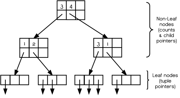
Figure 11: Hierarchical Positional Mapping.

We now describe hierarchical positional mapping, which is an indexing structure that adapts classical work on order-statistic trees [15]. Just like a typical B+ tree is used to capture the mapping from keys to records, we can use the same structure to map positions to tuple pointers. Here, instead of storing a key we store the count of elements stored within the entire sub-tree. The leaf nodes store tuple pointers, while the remaining store children pointers along with counts.

We show an example hierarchical positional mapping structure in Figure 11. Similar to a B+ tree of order $m$, our structure satisfies the following invariants. (i) Every node has at most $m$ children. (ii) Every non-leaf node (except root) as at-least $\left\lceil\frac{m}{2}\right\rceil$ children. (iii) All leaf nodes appear at the same level. Again similar to B+ tree, we ensure the invariants by either splitting or merging nodes, ensuring that the height of the tree is at most $\log_{\left\lceil m/2\right\rceil}N$.

Our hierarchical mapping structure makes accessing an item at the $n$th position efficient, by starting from the root node with $n^{\prime}=n$, and traversing downwards; at each node, given our current count $n^{\prime}$, we subtract the counts of as many of the children nodes from left-to-right (representing counts of sub-trees) as long as $n^{\prime}$ stays positive, and then follow the pointer to that child node, and repeat the process until we reach a leaf node and access a pointer to a tuple. Overall, the complexity of this operation is $\mathcal{O}(\log N)$. Insert/delete is similar, where we start at the appropriate leaf node (as before), insert or delete appropriate tuple pointers, and then update the counts of all nodes on the path to the modified leaf node. Once again, the complexity of this operation is $\mathcal{O}(\log N)$.

Overall, we find that the complexity of the hierarchical positional mapping is $\mathcal{O}(\log N)$ for all operations, while the Position-as-is approach has $\mathcal{O}(\log N)$ for access, but $\mathcal{O}(N\log N)$ for insert/delete. We empirically evaluate the impact of the difference in complexities in Section VII.

VI DataSpread Architecture

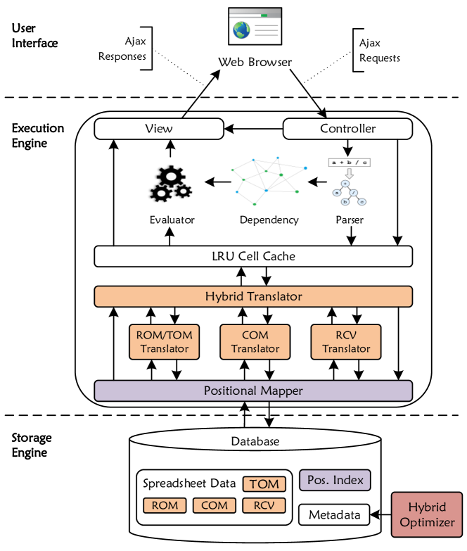
Figure 12: DataSpread Architecture.

We have implemented a fully functional DataSpread prototype as a web-based tool (using the open-source ZK Spreadsheet frontend [1]) on top of a PostgreSQL database. The prototype along with its source code, documentation, and user guide can be found at http://dataspread.github.io. Along with standard spreadsheet features, the prototype supports all the spreadsheet-like and database-like operations discussed in Section III. Screenshots of DataSpread in action can be found in our qualitative evaluation section (Section VII-D).

Fig. 12 illustrates DataSpread’s architecture, which at a high level can be divided into three main layers, (i) user interface, (ii) execution engine, and (iii) storage engine. The user interface consists of a spreadsheet widget, which presents a spreadsheet on a web-based interface and handles the interactions on it. The execution engine is a Java web application that resides on an application server. The controller accepts user interactions in form of events and identifies the corresponding actions, e.g., a formula update is sent to the formula parser, an update to a cell is sent to the cell cache. The dependency graph captures the formula dependencies between the cells and aids in triggering the computation of dependent cells. The positional mapper translates the row and column numbers into the corresponding stored identifiers and vice versa. The ROM/TOM, COM, RCV, and hybrid translators use their corresponding spreadsheet representations and provide a “collection of cells” abstraction to the upper layers. The TOM data model is handled as a special case of ROM. The hybrid translator is responsible for mapping the different regions on a spreadsheet to corresponding data models. ROM/TOM, COM, and RCV translators service getCells by using the tuple pointers, obtained from the positional mapper, to fetch required tuples. For a hybrid model, the mapping from a range to model is stored as metadata. The hybrid translator services getCells by identifying the responsible data model and delegating the call to it. Other operations such as cell updates are performed by the hybrid model in a similar fashion. This collection of cells are then cached in memory via an LRU cell cache. The storage engine consists of a database responsible for persisting data. This data is persisted using a combination of ROM, COM, RCV, and TOM (Section IV) along with positional mapping indexes, which map row/column numbers to tuple pointers (Section V), and metadata, which records information about the hybrid data model. The hybrid optimizer determines the optimal hybrid data model and is responsible for migrating data across data models.

Formula Evaluation. When a formula is entered a cell, the parser interprets it and identifies the cells required for its computation. The cell containing the formula is then said to be dependent on the cells required for its computation. The parser captures this dependency, i.e., the mapping between a cell and its dependent cells, in a so-called dependency graph. The evaluator fetches the cells required for computing the formula from the LRU cell cache in a read-through manner, i.e., the cache fetches the cells that are not present on demand from the underlying layer, and then computes the result of the formula. Finally, it persists the computed result by passing it back to the LRU cell cache in a write-through manner, i.e., the cache pushes its updates to the database via the hybrid translator. Whenever a user updates a cell, the evaluator uses the dependency graph to identify the cells that are dependent on the updated cell and triggers their computations. The triggered computations are performed by the evaluator and resultant values are persisted in the database by passing them to the LRU cell cache. If the resultant values are different from the old ones, then the evaluator triggers computation of the cells dependent on them, if any. The prototype also addresses a number of additional challenges especially related to efficient formula evaluation, including compact representation of formula dependencies, batched and lazy formula evaluation, and optimizing for user attention—these are important issues, but beyond the scope of this paper, which focuses on the storage engine.

Relational Operations. Since DataSpread is built on top of a traditional relational database, it leverages the SQL engine of the database and seamlessly supports SQL queries, via sql function, on the front-end spreadsheet interface. In addition, we support relational operators via the following spreadsheet functions: union, difference, intersection, crossproduct, join, filter, project, and rename. These functions return a single composite table value; to retrieve the individual rows and columns within that table value, we have an index(cell, i, j) function that looks up the (i, j)th row and column in the composite table value in location cell, and places it in the current location. See Appendix B for details.

VII Experimental Evaluation

In this section, we present an evaluation of the storage engine of DataSpread.

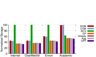
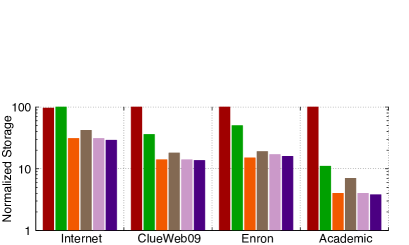
Figure 13: (a) Storage Comparison for PostgreSQL. (b) Storage Comparison on an Ideal Database.

(a)

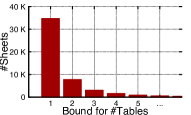
(b)

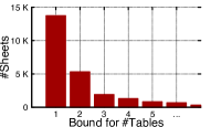
(c)

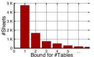
(d)

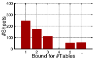
Figure 14: Upper bound for #Tables in the optimal decomposition — (a) Internet. (b) ClueWeb09. (c) Enron. (d) Academic.

VII-A Experimental Setup

Environment. We have implemented the data models and positional mapping techniques using PostgreSQL 9.6, configured with default parameters. We run all of our experiments on a workstation running Windows 10 on an Intel Core i7-4790K 4.0 GHz with 16 GB RAM. Our test scripts are single-threaded applications developed in Java. While we have a fully functional prototype, our test scripts are independent of it, so that we can isolate the back-end performance implications. We ensured fairness by clearing the appropriate cache(s) before every run.

Datasets. We evaluate our algorithms on a variety of real and synthetic datasets. Our real datasets are the ones listed in Table I. To test scalability, since our real-world datasets limited in scale by what current spreadsheet tools can support, we constructed large synthetic spreadsheet datasets. We identify several goals for our experimental evaluation:

Goal 1: Presentational Awareness and Access on Real and Synthetic Datasets. We evaluate the hybrid data models selected by our algorithms against the primitive data models, when the cost model is optimized for storage. We compare our algorithms: DP (Section IV-D), and Greedy and Agg (greedy and aggressive-greedy from Section IV-E) against ROM, COM, and RCV, which represent our best current database approach. We evaluate these data models on both storage, as well as formulae access cost, based on the spreadsheet formulae. In addition, we evaluate the running time of the hybrid optimization algorithms for DP, Greedy, and Agg.

Goal 2: Presentational Access (With Updates) on Synthetic Datasets. We evaluate the impact of our positional mapping schemes in aiding access on the spreadsheet. We focus on Position-as-is, Monotonic, and Hierarchical positional mapping schemes (introduced later) applied on the ROM primitive model, and evaluate the performance of fetch, insert, and delete operations on varying the number of rows.

Goal 3: Qualitative Evaluation. We evaluate the user experience of DataSpread relative to Excel, and study whether DataSpread’s storage engine enables users to effectively work with large datasets in two different scenarios.

Other Experiments. In the Appendix, we present a number of other complementary experiments, including (i) Goal 1: a drill-down into the performance of hybrid data models (Appendix C-A1); (ii) Goal 2: an investigation of incremental maintenance of hybrid data models (Appendix C-A2); (iii) Goal 3: a study on varying parameters of synthetic spreadsheets on positional mapping (Appendix C-B1).

VII-B Presentational Awareness and Access

Takeaway: Hybrid data models provide substantial benefits over primitive data models, with up to 20% reductions in storage, and up to 50% reduction in formula evaluation time on PostgreSQL on real and synthetic spreadsheet datasets, compared to the best primitive data model. While DP has better performance on storage than Greedy and Agg, it suffers from high running time; Agg bridges the gap between Greedy and DP, while taking only marginally more running time than Greedy; both Agg and Greedy are within 10% of the optimal storage. Lastly, if we were to design a database storage engine from scratch, the hybrid data models would provide up to 50% reductions in storage compared to the best primitive data model. Overall, our hybrid data models bring scalability to spreadsheets: efficiently support storage across a range of spreadsheet structures, and access data via position in an efficient manner.

The goal of this section is to evaluate presentational access and awareness (without updates) by evaluating our data models—on real and synthetic datasets.

a. Real Dataset: Storage Evaluation on PostgreSQL. We begin with an evaluation of storage for different data models on PostgreSQL. The costs for storage on PostgreSQL as measured by us is as follows: $s_{1}$ is $8$ KB, $s_{2}$ is $1$ bit, $s_{3}$ is $40$ bytes, $s_{4}$ is $50$ bytes, and $s_{5}$ (RCV’s tuple cost) is $52$ bytes. We plot the results in Figure 13(a): here, we depict the average normalized storage across sheets; in addition to the aforementioned data models, we also plot a lower bound for the optimal hybrid data model (denoted OPT)—the cost of storing only non-empty cells in a single ROM, i.e., the cost ignoring the overhead of extra tables and empty cells. For Internet, ClueWeb09, and Enron, we found RCV to have the worst performance, and hence normalized it to a cost of 100, and scaled the others accordingly; for the Academic datasets, we found COM to have the worst performance, and hence normalized it to a cost of 100, and scaled the others. The first three datasets are primarily used for data sharing, and as a result are quite dense. As a result, ROM and COM do well, using about 40% of the storage of RCV. At the same time, DP, Greedy and Agg perform roughly similarly, and better than the primitive data models, providing an additional reduction of 15-20%. On the other hand, the last dataset, which is primarily used for computation, and is very sparse, RCV does better than ROM and COM, while DP, Greedy, and Agg once again provide additional benefits. We finally observe that DP, Greedy, and Agg are all very close (within $10\%$) of OPT. From this we conclude that the solution give by Agg is close to the optimal in terms of cost.

We next show that the error bound of using a recursive decomposition based algorithms (DP, Greedy, and Agg) is small as compared to the optimal solution. For this we plot the upper bound for the number of tables in the optimal solution, i.e., $\sum\left\lfloor\frac{e\times s_{2}}{s_{1}}+1\right\rfloor$, for the four data sets in Figure 14. Here, we observe the the number of tables in the optimal solution is typically small – $90\%$ of spreadsheets have fewer than $10$ tables in the optimal decomposition. From the above observation and Theorem 3, we conclude that the error bound of using the search space of recursive decomposition for practical purposes is small.

b. Real Dataset: Storage Evaluation on an Ideal Database. Note that the reason why RCV does so poorly for the first three datasets is because PostgreSQL imposes a high overhead per tuple, of 50 bytes, considerably larger than the amount of storage per cell. So, to explore this further, we investigated the scenario if we could redesign our database storage engine from scratch. We consider a theoretical “ideal” cost model, where the cost of a ROM or COM table is equal to the number of cells, plus the length and breadth of the table (to store the data, the schema, as well as position), while the cost of an RCV row is simply 3 units (to store the data, as well as the row and column number). We plot the results in Figure 13(b) in log scale for each of the datasets—we exclude COM for this chart since it is identical to ROM. Here, we find that ROM has the worst cost since it no longer leverages benefits from minimizing the number of tuples. (For Internet, ROM and RCV are similar, but RCV is slightly worse.) As before, we normalize the cost of the worst model to 100 for each sheet, and scaled the others accordingly. As an example, we find that for the ClueWeb09 corpus, RCV, DP, Greedy and Agg have normalized costs of about 36, 14, 18, and 14 respectively—with the hybrid data models more than halving the cost of RCV, and getting $\frac{1}{7}^{th}$ the cost of ROM. Furthermore, DP provides additional benefits relative to Greedy, and Agg ends up bringing us close to DP performance; finally, we find that Agg and DP are both very close to OPT (within $10\%$).

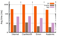
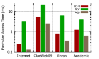
Figure 15: (a) Hybrid optimization algorithms: Running time. (b) Average access time for formulae.

Figure 16: Genomics Use Case: VCFs in DataSpread.

c. Real Dataset: Running Time of Hybrid Optimization Algorithm. Our next question is how long our hybrid data model optimization algorithms for DP, Greedy, and Agg, take on real datasets. In Figure 15(a), we depict the average running time on the four real datasets. The results for all datasets are similar, e.g., for Enron, DP took 6.3s on average, Greedy took 45ms (a 140$\times$ reduction), while Agg took 345ms (a 20$\times$ reduction). Thus DP has the highest running time for all datasets, since it explores the entire space of models that can be obtained by recursive partitioning. Between Greedy and Agg, Greedy turns out to take less time. Note that these observations are consistent with our complexity analyses from Section IV-E. That said, Agg allows us to trade off running time for improved performance on storage (as we saw earlier). Greedy takes less time than Agg; but Agg allows us to trade off running time for improved performance on storage. Between Greedy and Agg, Greedy turns out to take less time. Note that these observations are consistent with our complexity analyses from Section IV-E. That said, Agg allows us to trade off running time for improved performance on storage (as we saw earlier). We note that for the cases where the spreadsheets were large, we terminated DP after about 10 minutes, since we want our optimization to be relatively fast. (Note that using a similar criterion for termination, Agg and Greedy did not have to be terminated for any of the real datasets.) To be fair across all the algorithms, we excluded all of these spreadsheets from this chart—if we had included them, the difference between DP and the other algorithms would be even more stark.

d. Real Dataset: Formulae Access Evaluation on PostgreSQL. We next evaluate if our hybrid data models, optimized only on storage, have any impact on the access cost for spreadsheet formulae. Our hope is that spreadsheet formulae focus on “tightly coupled” tabular areas, which our hybrid data models are able to capture and store in separate tables. For this evaluation, we focus on Agg, since it provided the best trade-off between running time and storage costs. Given a sheet in a dataset, for each data model, we measured the time taken to evaluate the formulae in that sheet, and averaged this time across all sheets and all formulae. We plot the results in Figure 15(b) in log scale in ms. As a concrete example, on Internet, ROM has a formula access time of 0.23, RCV has 3.17, and Agg has 0.13. Thus, Agg provides a substantial reduction of 96% over RCV and 45% over ROM—even though Agg was optimized for storage and not for formula access. This validates our design of hybrid data models to store spreadsheet data. Note that while the performance numbers for the real spreadsheet datasets are small for all data models (due to the size limitations in present spreadsheets), when scaling up to large datasets, and formulae on them, these numbers will increase in proportionally, at which point it is even more important to opt for hybrid data models, as we will see next.

(a)

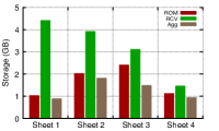
(b)

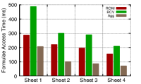
Figure 17: Synthetic sheets (a) Storage. (b) Access time.

e. Synthetic Dataset: Storage and Formula Access Evaluation We now run our tests on large synthetic spreadsheets with 100+ million cells to evaluate our techniques in large dataset scenarios. We create synthetic spreadsheets by populating an empty sheet with twenty dense rectangular regions to simulate randomly placed tables. We add $100$ randomly generated formulae that access rectangular ranges of these tables. Figures 17(a) and 17(b) depict the storage requirements and the formulae access time respectively for four synthetic spreadsheets, which are in the decreasing order of density (the fraction of cells that are filled-in in the minimum bounding rectangle). For both storage and access, we find that Agg is better than ROM, which is better than RCV; as density is decreased, RCV’s performance becomes closer to ROM. Agg performs the best, providing substantial reductions of up to 50-75% of the time taken for access with ROM or RCV.

(a)

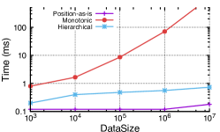
(b)

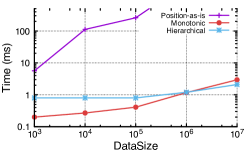
(c)

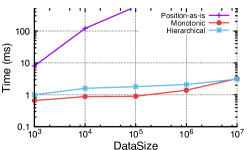
Figure 18: Positional mapping performance for (a) Select. (b) Insert. (c) Delete.

VII-C Presentational Access with Updates

Takeaway: Hierarchical positional mapping retains the rapid fetch benefits of position-as-is, while also providing rapid inserts and updates. Thus, hierarchical positional mapping is able to perform positional operations within a few milliseconds, while the other schemes often take seconds on large datasets. Overall, our hierarchical positional mapping schemes support presentational access with updates, validating the fact that our storage engine can support interactivity.

We now evaluate presentational access (with updates) by studying our positional mapping methods (Section V) on synthetic datasets. We compare our hierarchical positional mapping scheme (denoted hierarchical), with position as-is (denoted position-as-is): this is the approach a traditional database with a B+ tree would use. In addition, motivated by the online dynamic reordering technique in Raman et al. [32], we consider another baseline (denoted monotonic), where we store a monotonically increasing sequence of identifiers (with gaps) to capture the position. Using this sequence we dynamically order the tuples at run-time (by sorting); whereas the gaps in the sequence enable efficient insert/delete operations. The dynamic reordering sacrifices the performance of the fetch operation as it needs to discard $n-1$ tuples to fetch $n^{th}$ tuple.

We operate on a dense synthetic dataset ranging from $10^{3}$ to $10^{7}$ rows, with $100$ columns with all cells filled; and repeat this $1000$ times. We evaluate the performance of a single ROM table with all of the data; evaluations for other data models are similar. Figure 18 displays the average time taken to perform a fetch, insert, and delete of a single (random) row.

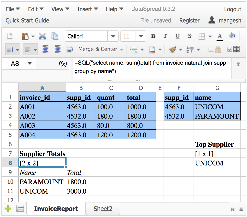
Figure 19: Customer Management in DataSpread.

We see that position-as-is performs well for fetch. However, the insert and delete time increases rapidly with the data size, due to cascading updates; thus, beyond a data size of $10^{5}$, position-as-is is no longer interactive ($>500ms$) for insert and delete. Conversely, the response time of monotonic for fetch increases rapidly with data size. This is again expected, as we need to linearly search through the monotonic keys to retrieve the required records—making it infeasible for large datasets. Lastly, we find that hierarchical performs well for all operations and performance does not get degrade even with data sizes of $10^{9}$ tuples. In comparison with the other schemes, hierarchical performs all of the three aforementioned operations in few milliseconds, which makes it the practical choice for presentational access with updates.

VII-D Qualitative Evaluation

We now evaluate DataSpread to see how it can handle the use cases described in Section I. With our genomics use case, we evaluate the scalability of DataSpread, and with our customer management use case, we evaluate the functionality.

a. Evaluating Scale for Genomics: For this evaluation, we used a VCF file provided by our biology collaborators, as described in Example $1$, and used it to perform basic exploration. We contrast the performance of DataSpread with Excel. Our VCF file has 1.3M rows and 284 columns. Unfortunately, we were unable to load this file in Excel since it exceeds Excel’s limits. Importing the file in DataSpread takes about a minute. On the other hand, even after reducing the VCF file to 1M rows, Excel is unable to import the file within an hour. After substantially reducing the file size to 130K rows, we were able to import it into Excel in about $10$ minutes. After loading the 1.3M VCF file, we were able to take advantage of DataSpread’s efficient positional access to scroll up and down to explore the data with interactive (sub-second) response times. Figure 16 shows a screenshot of the file in DataSpread, having scrolled to the millionth row.

Takeaway: DataSpread enables users to interactively work on large spreadsheets that main-memory based spreadsheet applications are unable to handle.

b. Evaluating Functionality for Customer Management: For evaluating functionality, as described in Example $2$, we leverage the database-oriented operations discussed in Section III. Using linkTable, we first establish a two-way synchronization between the spreadsheet regions and the invoice and supp tables in the database (Figure 19). These linked regions enable us to directly manipulate the underlying tables via spreadsheet operations such as cell updates; this is not possible in spreadsheet tools that only allow one-way import of data from a backend database to a spreadsheet. We used the sql function in cell A8 to join the two tables and perform grouping and aggregation; this is less cumbersome and more efficient compared to Excel’s vlookup and pivot tables, and indexed into the composite value in A8 to display the results in A9:B11. Finally, we use the project and select functions to get the top supplier in cell G8; any updates to the underlying tables are automatically reflected in the function’s output.

Takeaway: The direct manipulation and database-oriented features of DataSpread enable interactive management of data via database tables on a spreadsheet interface.

VIII Related Work

Our work draws on related work from multiple areas: (i) that enhance database usability, (ii) those that attempt to merge spreadsheet and database functionalities, but without a holistic integration, and (iii) order or array-based database management systems. We described our vision for DataSpread in an earlier demo paper [7].

1. Making databases more usable. There has been a lot of recent work on making database interfaces more user friendly [2, 20]. This includes recent work on gestural query and scrolling interfaces [30, 29, 28, 35, 19], visual query builders [11, 3], query sharing and recommendation tools [21, 12, 22], schema-free databases [31], schema summarization [48], and visual analytics tools [9, 27, 36, 18]. However, none of these tools can replace spreadsheet software which has the ability to analyze, view, and modify data via a direct manipulation interface [34] and has a large user base—this paper aims to make this interface available to manipulate databases.

2a. One-way import of data from databases to spreadsheets. There are various mechanisms for importing data from databases to spreadsheets, and then analyzing this data within the spreadsheet. This approach is followed by Excel’s Power BI tools, including Power Pivot [44], with Power Query [45] for exporting data from databases and the web or deriving additional columns and Power View [45] to create presentations; and Zoho [41] and ExcelDB [43](on Excel), and Blockspring [42] enabling the import from a variety of sources including the databases and the web. Typically, the import is one-shot, with the data residing in the spreadsheet from that point on, negating the scalability benefits from the database. Indeed, Excel 2016 specifies a limit of 1M records that can be imported, illustrating that the scalability benefits are lost. Zoho specifies a limit of 0.5M records. Furthermore, the connection to the base data is lost: modifications made at either end are not propagated.

2b. One way export of operations from spreadsheets to databases. There has been some work on exporting spreadsheet operations into database systems, such as Oracle [46, 47], 1010Data [39] and AirTable [40], to improve the performance of spreadsheets. However, the database itself has no awareness of the existence of the spreadsheet, making the integration superficial. In particular, positional and ordering aspects are not captured, and user operations on the front-end, e.g., inserts, deletes, and adding formulae, are not supported. Indeed, the lack of awareness makes the integration one-shot, with the current spreadsheet being exported to the database, with no future interactions supported at either end: thus, in a sense, the interactivity is lost. Other efforts in this space include that by Cunha et al. [17] to recognize functional dependencies in spreadsheets. Other work has examined the extraction of structured relational data from spreadsheets [13, 14].

2c. Using a spreadsheet to mimic a database. There has been some work on using a spreadsheet to pose as traditional database. E.g., Tyszkiewicz [37] describes how to simulate database operations in a spreadsheet. However, this approach loses the scalability benefits of relational databases. Bakke et al. [6, 5, 4] support joins by depicting relations using a nested relational model. Liu et al. [26] use spreadsheet operations to specify single-block SQL queries; this effort is essentially a replacement for visual query builders. Recently, Google Sheets [38] has provided the ability to use single-table SQL on its frontend, without availing of the scalability benefits of database integration. Excel, with its Power Pivot and Power Query [45] functionality has made moves towards supporting SQL in the front-end, with the same limitations. Like this line of work, we support SQL queries on the spreadsheet frontend, but our focus for this paper is on representing and operating on spreadsheet data within a database.

3. Order-aware database systems. Some limited aspect of presentational awareness, in particular, order, has been studied. The early work of online dynamic reordering [32] supports data reordering based on user preference, citing a spreadsheet-like interface [33] as an application. More recently, there has been work on array-based databases, but most of these systems do not support edits, e.g., SciDB [8] supports an append-only, no-overwrite data model.

IX Conclusions

We introduced our vision of presentational data management: building a system that holistically integrates spreadsheets and databases. We focused on developing a storage engine for our PDM prototype DataSpread, characterizing key requirements in the form of presentational awareness and access. We addressed presentational awareness by proposing three primitive data models for representing spreadsheet data, along with algorithms for identifying optimal hybrid data models from recursive decomposition. Our hybrid data models provide substantial reductions in terms of storage (up to 20–50%) and formula evaluation (up to 50%) over the primitive data models. For presentational access, we couple our hybrid data models with a hierarchical positional mapping scheme, making working with large spreadsheets interactive. Overall, DataSpread emerges as a promising solution for interactively analyzing, manipulating, and managing large datasets.

Appendix A Hybrid Decomposition Details

A-A Hybrid Decomposition: Hardness

Here, we demonstrate that Problem 1 is NP-Hard; for the decision version of the problem, a value $k$ is provided, and the goal is to test if there is a hybrid data model with $\operatorname{cost}(T)\leq k$.

We use a reduction from the minimum edge length partitioning problem of rectilinear polygons [25]. A rectilinear polygon is one in which all edges are either aligned with the $x$-axis or the $y$-axis. The minimality criterion is the total length of the edges (lines) used to form the internal partition. Notice that this doesn’t necessarily correspond to the minimality criterion of reducing the number of components. We illustrate this in Figure 20, which is borrowed from the original paper [25]. The following decision problem was shown to be NP-Hard in [25]: Given any rectilinear polygon $P$ and a number $k$, is there a rectangular partitioning whose total edge length does not exceed $k$?

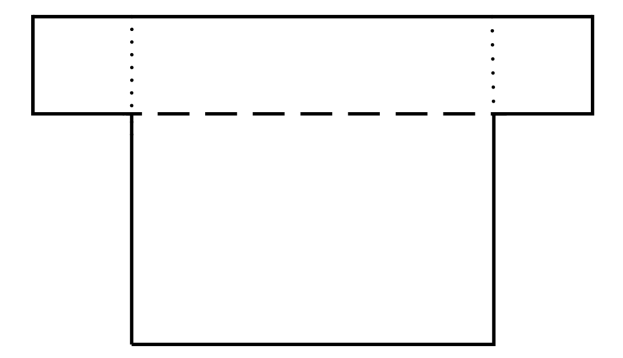
Figure 20: Minimum number of rectangles (– – –) does not coincide with minimum edge length ($\cdots$).

Proof:

Consider an instance $P$ of the polygon partitioning problem with minimum edge length required to be at most $k$. We now represent the polygon $P$ in a spreadsheet by filling the cells interior of the polygon with arbitrary values, and not filling any other cell in the spreadsheet. Let $C=\{C_{1},C_{2},\ldots,C_{m}\}$ represent the set of all filled cells in the spreadsheet. We claim that a minimum edge length partition of the given rectilinear polygon $P$ of length at most $k$ exists iff there is a solution for the following setting of the optimal hybrid data model problem: $s_{1}=0,s_{2}=2|C|+1,s_{3}=s_{4}=1$, where the storage cost should not exceed $k^{\prime}=k+\frac{\operatorname{Perimeter}(P)}{2}+(2|C|+1)|C|$ for some decomposition of the spreadsheet.

$\Rightarrow$ Say the spreadsheet we generate using $P$ has a decomposition of rectangles whose storage cost is less than $k^{\prime}=k+\frac{\operatorname{Perimeter}(P)}{2}+s_{2}|C|$. We have to show that there exists a partition with minimum edge length of at most $k$.

First, notice that there exists a valid decomposition that doesn’t store any blank cell. Say there is a decomposition that stores a blank cell. Since we are now storing $|C|+1$ cells at minimum, $k^{\prime}>s_{2}(|C|+1)=|C|s_{2}+s_{2}=|C|s_{2}+2|C|+1$ and thus $k^{\prime}>|C|(s_{2}+1+1)$, which is the cost of storing each cell in a separate table. Therefore, if we have a decomposition that stores a blank cell, we also have a decomposition that does not store any blank cell and has lower cost. Second, there exists a decomposition of the spreadsheet where all the tables are disjoint. The argument is similar to the previous case since storing the same cell twice in different tables is equivalent to storing an extra blank cell.

From our above two observations, we conclude that there exists a decomposition where all tables are disjoint, and no table stores a blank cell. Therefore, this decomposition corresponds to partitioning the given spreadsheet into rectangles. We represent this partition of the spreadsheet by $T=\{T_{1},T_{2},\ldots,T_{p}\}$. We now show that this partition of the spreadsheet corresponds to a partitioning of the rectilinear polygon $P$ with edge-length less than $k$. On setting $s_{1}=0,s_{2}=2|C|+1,s_{3}=s_{4}=1$, we get:

$$\operatorname{cost}(T) =\sum_{i=1}^{p}0+s_{2}|C|+1\cdot\left(\sum_{i=1}^{p}c_{i}+\sum_{i=1}^{p}r_{i}\right)$$ (5)

since $$\operatorname{cost}(T)\leq k^{\prime}=k+\frac{\operatorname{Perimeter}(P)}{2}+s_{2}|C|$$,

$$\sum_{i=1}^{p}(r_{i}+c_{i})\leq k+\frac{\operatorname{Perimeter}(P)}{2}$$ (6)

$$\sum_{i=1}^{p}\frac{\operatorname{Perimeter}(T_{i})}{2}\leq k+\frac{\operatorname{Perimeter}(P)}{2}$$ (7)

$$\implies \sum_{i=1}^{p}\operatorname{Perimeter}(T_{i})\leq 2\times k+\operatorname{Perimeter}(P)$$ (8)

Since the sum of perimeters of all the tables $T_{i}$ counts the boundary of $P$ exactly once, and the edge length partition of $P$ exactly twice, the partition of the spreadsheet $T=\{T_{1},T_{2},\ldots,T_{p}\}$ corresponds to an edge-length partitioning of the given rectilinear polygon $P$ with edge-length less than $k$.

$\Leftarrow$ Let us assume that the given rectilinear polygon $P$ has a minimum edge length partition of length at most $k$. We have to show that there exists a decomposition of the spreadsheet whose storage cost is at most $k^{\prime}=k+\frac{\operatorname{Perimeter}(P)}{2}+s_{2}|C|$. Let us represent the set of rectangles that corresponds to an edge length partition of $P$ of at most $k$ as $T=\{T_{1},T_{2},\ldots,T_{p}\}$. We shall use the partition $T$ of $P$ as the decomposition of the spreadsheet itself:

$$\operatorname{cost}(T)=\sum_{i=1}^{p}s_{1}+s_{2}\cdot(r_{i}\times c_{i})+s_{3}\cdot c_{i}+s_{4}\cdot r_{i}$$ (9)

$$\operatorname{cost}(T)=\sum_{i=1}^{p}s_{1}+s_{2}\sum_{i=1}^{p}\cdot(r_{i}\times c_{i})\\ +s_{3}\sum_{i=1}^{p}c_{i}+s_{4}\sum_{i=1}^{p}r_{i}$$ (10)

substituting $s_{1}=0,s_{2}=2|C|+1,s_{3}=s_{4}=1$, we get:

$$\operatorname{cost}(T)=\sum_{i=1}^{p}0+s_{2}|C|+1\cdot\left(\sum_{i=1}^{p}c_{i}+\sum_{i=1}^{p}r_{i}\right)$$ (11)

$$\operatorname{cost}(T)=s_{2}|C|+\sum_{i=1}^{p}(r_{i}+c_{i})$$ (12)

$$\operatorname{cost}(T)=s_{2}|C|+\sum_{i=1}^{p}\frac{\operatorname{Perimeter}(T_{i})}{2}$$ (13)

since $\sum_{i=1}^{p}\operatorname{Perimeter}(T_{i})=2\times k+\operatorname{Perimeter}(P)$, we have:

$$\operatorname{cost}(T)=s_{2}|C|+k+\frac{\operatorname{Perimeter}(P)}{2}=k^{\prime}$$ (14)

$\implies\operatorname{cost}(T)=k^{\prime}$

Therefore, the decomposition of the spreadsheet using $T$ corresponds to a decomposition whose storage cost equals $k^{\prime}$. Note that our reduction can be done in polynomial time. Therefore we can solve the minimum length partitioning problem in polynomial time, if we have a polynomial time solution to the optimal storage problem. However, since the minimum length partitioning problem is NP-Hard [25], the optimal hybrid data model problem is NP-Hard. This completes our proof. ∎

Hardness Results for Extensions. So far, we have only considered the ROM data model for our tables, and assume that data is duplicated when two tables overlap. It can be shown that even when we extend to the case when RCV is permitted, and when we allow data to be represented in multiple tables, the problem continues to be NP-Hard. For each case we consider, we restrict our argument to an outline of the proof since it largely mimics what is presented for the basic case.

ROM and RCV; without data overlap. Now, we consider the following problem. Given a spreadsheet with data, our goal is to decompose the spreadsheet into tables (using ROM and RCV) such that the overall storage cost is minimized, with no two tables overlapping with each other.

(Proof sketch) Our basic idea is to achieve two goals: (i) ensure that the blank cells in the spreadsheets aren’t stored in any table and (ii) ensure that we always prefer ROM over RCV, since we can then employ our proof for Problem 1.

We achieve goal 1 by setting $s_{2}=\infty$ in our cost model, and goal 2 by setting $s_{1}=0$, $s_{3}=1$, and $s_{4}=1$ as before. We now use a reduction from minimum edge length partitioning problem of rectilinear polygons [25] as before to show hardness. Note that if we allow tables to overlap, and when they do, if we duplicate the data in the overlapping cells in both tables, setting $s_{1}=0,s_{2}=\infty,s_{3}=1$, and $s_{4}=1$ can lead to a reduction from the minimum edge length partitioning problem of rectilinear polygons to show hardness. The same proof as for Problem 1 continues to hold.

ROM with overlap; without data duplication. Now, we consider a variant of the previous setting: when the tables overlap, we do not duplicate the same cell’s value in two different tables. Note that this is different from earlier formulations, where we indeed duplicated data across overlapping tables.

(Proof sketch) Our basic idea is to achieve to achieve two goals: (i) ensure that blank cells aren’t stored in any table and (ii) only the number of rectangles, i.e., tables, we have matters, not their dimensions.

We achieve goal 1 by setting $s_{2}=\infty$ in our cost model, and goal 2 by setting $s_{3}=0$ and $s_{4}=0$. We have $s_{1}=1$. We now use a reduction from the rectangle covering problem [16] to show hardness. The reduction is straightforward since we are essentially minimizing the number of tables to cover all of the filled cells in the sheet, which is exactly what the rectangle covering problem aims to minimize.

A-B Hybrid Decomposition: DP Bound

Approximation Bound for DP. Here, we obtain an approximation bound for our dynamic programming formulation discussed in Section IV-D. Say we have $k$ rectangles in the optimal decomposition; with storage cost $c$. Then, we show that the dynamic programming algorithm, which explores the entire space of models obtained from recursive decomposition, identifies a decomposition with a cost that is at most $c+s_{1}\times\frac{k(k-1)}{2}$, where $s_{1}$ is the cost of storing a new table as in Equation 1.

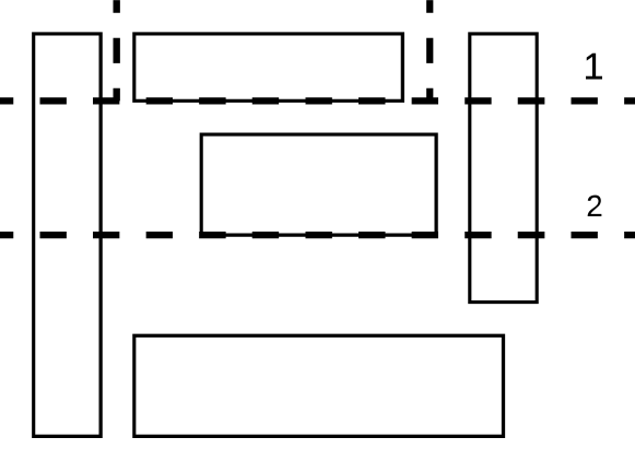
Figure 21: Obtaining a recursive decomposition from the optimal solution.

Proof:

Let the optimal decomposition consist of a set of five rectangles $R$ as in Figure 21. Starting from $R$, we will construct a recursive decomposition solution with cost $c+s_{1}\times\frac{k(k-1)}{2}$, denoted as $R^{\prime}$, using the following steps. Sort the rectangles from the optimal solution in the increasing order of their bottom edge. Pick the first rectangle, and use a line through its bottom edge to cut or partition the remaining rectangles. This is the first “partitioning” step, denoted as 1 in Figure 21. This partitioning step leads to two portions. We handle the top portion with vertical partitions, while for the bottom portion we recurse. This partition introduces at most $k-1$ new rectangles in the top half and eliminates one rectangle.

Thus, at every step, we have $k-1$ new rectangles and reduce the total number of rectangles by $1$. That is, the next partition will introduce at most $k-2$ rectangles; and so on. So, we in total we $(k-1)+(k-2)+\ldots+1=\frac{k(k-1)}{2}$ new rectangles. Since the dynamic programming algorithm explores the entire space of recursive decomposition based data models, it also considers $R^{\prime}$ as one of the candidates. Thus; its solution must be at least as good. Hence proved. ∎

Bound for number of Tables. Since the bound given by Theorem 3 and proved above is an additive bound in terms of number of tables, we use Theorem 4 to show that practically the number of tables in the optimal decomposition is small; thereby enabling us to claim that our dynamic programming solution is not too far from optimal. Here, we show that the optimal solution to Problem 1 for a minimum bounding rectangle of a connected component will have at most $\left\lfloor\frac{e\times s_{2}}{s_{1}}+1\right\rfloor$ rectangles, where $e$ is the number of empty cells in the bounding rectangle.

Proof:

Let the optimal decomposition for a minimum bounding rectangle of a connected component $C$ have $k^{\prime}$ tables. Therefore, we have the cost representing the minimum bounding rectangle using a single table is higher than the optimal decomposition into $k^{\prime}$ tables, i.e.,

$$\sum_{i=1}^{k^{\prime}}s_{1}+s_{2}\cdot(r_{i}\times c_{i})+s_{3}\cdot c_{i}+s_{4}\cdot r_{i}\leq\\ s_{1}+s_{2}\cdot(r_{0}\times c_{0})+s_{3}\cdot c_{0}+s_{4}\cdot r_{0},$$ (15)

where $r_{1},..,r_{k^{\prime}}$ and $c_{1},..,c_{k^{\prime}}$ are the number of rows and columns respectively for each of the tables in the optimal decomposition and $r_{0}$ and $c_{0}$ are number of rows and columns for the minimum bounding rectangle.

Since our region of focus is a minimum bounding rectangle encapsulating a connected component, we do not have any empty rows or columns. Thus, each row and column should be captured by at least one rectangle in the optimal decomposition. Hence, we have,

$$\sum_{i=1}^{k}s_{3}\cdot c_{i}+s_{4}\cdot r_{i}\geq s_{3}\cdot c_{0}+s_{4}\cdot r_{0}$$ (16)

Subtracting Equation 16 from 15 we have,

$$\sum_{i=1}^{k}s_{1}+s_{2}\cdot(r_{i}\times c_{i})\leq s_{1}+s_{2}\cdot(r_{0}\times c_{0}).$$ (17)

Since the optimal solution should represent all the filled-in cells at least once, we have $\sum_{i=1}^{k}(r_{i}\times c_{i})\geq r_{0}\times c_{0}-e$, where $e$ is the number of empty cells in the bounding box. Subtracting this from Equation 17 and simplifying, we get

$$k\cdot s_{1} \leq s_{1}+e\times s_{2}.$$ (18)

$$k \leq 1+\frac{e\times s_{2}}{s_{1}}.$$ (19)

Since $k$ is an integer, we have

$$k \leq\left\lfloor 1+\frac{e\times s_{2}}{s_{1}}\right\rfloor.$$ (20)

Hence proved. ∎

A-C Hybrid Data Model: Extensions

In this section, we discuss a number of extensions to the cost model of the hybrid data model. We will describe these extensions to the cost model, and then describe the changes to the basic dynamic programming algorithm; modifications to the greedy and aggressive greedy decomposition algorithms are straightforward.

A-C1 RCV, COM and TOM

The cost model can be extended in a straightforward manner to allow each rectangular area to be a ROM, COM, or an RCV table. (We deal with the TOM case later.) First, note that it doesn’t benefit us to have multiple RCV tables—we can simply combine all of these tables into one, and assume that we’re paying a fixed up-front cost to have one RCV table. Then, the cost for a table $T_{i}$, if it is stored as a COM table is:

$$\operatorname{comCost}(T_{i})=s_{1}+s_{2}\cdot(r_{i}\times c_{i})+s_{4}\cdot c_{i}+s_{3}\cdot r_{i}.$$

This equation is the same as Equation 1, but with the last two constants transposed. And the cost for a table $T_{i}$, if it is stored as an RCV table is simply:

$$\operatorname{rcvCost}(T_{i})=s_{5}\times\#\text{cells}.$$

where $s_{5}$ is the cost incurred per tuple. Once we have this cost model set up, it is straightforward to apply dynamic programming once again to identify the optimal hybrid data model encompassing ROM, COM, and RCV. The only step that changes in the dynamic programming equations is Equation 2, where we have to consider the COM and RCV alternatives in addition to ROM. To handle TOM tables, we assume that the corresponding cells are empty; while also setting the $\operatorname{romCost}($) and $\operatorname{comCost}($) of any tables overlapping with these cells as $\infty$. We have the following theorem.

Theorem 6 (ROM, COM, TOM, and RCV).

The optimal ROM, COM, TOM, and RCV-based hybrid data model based on recursive decomposition can be determined in PTIME.

A-C2 Incremental Decomposition

So far, we have focused on finding an optimal decomposition given a static spreadsheet. We now consider how we can support incremental maintenance of the decomposition across updates. Here, along with the storage cost, we also consider the cost of migrating cells from an existing decomposition $T_{o}$ to a new decomposition $T$. We define the migration cost as $\operatorname{migCost}((x_{1},y_{1}),(x_{2},y_{2}))=\#\text{cells}$, where $\#\text{cells}$ denotes the number of populated cells in the rectangular region defined by $(x_{1},y_{1}),(x_{2},y_{2})$. To migrate a region of a spreadsheet into a new decomposition, we assume that we only use an existing table if it exactly covers the region; for all other cases we migrate all of the populated cells within the region to the new decomposition. In other words, we do not consider the cases when an existing table needs to be modified either to accommodate or eliminate rows or columns. We introduce a factor $\eta$ to enable users to balance the trade-off between the migration cost and storage cost; our objective is thus find a data model $T$ such that $\operatorname{cost}(T)+\eta\cdot\operatorname{migCost}()$ is minimized.

For incremental decomposition, we update the dynamic programming formulation by adding an additional case that retains the decomposition as is and updates the $\operatorname{romCost}()$ to include the migration cost in terms of the number of cells that need to be migrated from the existing model into a new model. As the migration cost for a region is defined as the number of populated cells, the migration cost of a region can be computed independently of the remaining regions. This enables us to employ dynamic programming once again.

• Keep the decomposition as-is. This is permissible only if the there exists a ROM model at $(x_{1},y_{1}),(x_{2},y_{2})$ in $T_{o}$.

  $$\operatorname{romCost}((x_{1},y_{1}),(x_{2},y_{2}))=\\ s_{1}+s_{2}\cdot(r_{12}\times c_{12})+s_{3}\cdot c_{12}+s_{4}\cdot r_{12},$$ (21)

• Store the area as ROM by migrating the non-empty cells into the new model.

  $$\operatorname{romCost}((x_{1},y_{1}),(x_{2},y_{2}))=s_{1}+s_{2}\cdot(r_{12}\times c_{12})+\\ s_{3}\cdot c_{12}+s_{4}\cdot r_{12}+\eta\cdot\operatorname{migCost}((x_{1},y_{1}),(x_{2},y_{2}))$$ (22)

Note that we may be able to migrate a region more efficiently by leveraging existing tables that partially cover the region; however, this will lead to complications in leveraging tables that span more than one region, and any reorganization costs involved. For simplicity, we do not consider such migrations. As we will demonstrate in Appendix C, this still leads to adequate performance.

A-C3 Access Cost.

So far, we have only been focusing on storage. Our cost model can be extended in a straightforward manner to handle access cost—both scrolling-based operations, and formulae, and our dynamic programming algorithms can similarly be extended to handle access cost without any substantial changes. We focus on formulae since they are often the more substantial cost of the two; scrolling-based operations can be similarly handled. For formulae, there are multiple aspects that contribute to the time for access: the number of tables accessed, and within each table, since data is retrieved at a tuple level, the number of tuples that need to be accessed, and the size of these tuples. Once again, each of these aspects can be captured within the cost model via constants similar to $s_{1},\ldots,s_{5}$, and can be seamlessly incorporated into the dynamic programming algorithm. Thus, we have:

Theorem 7 (Optimality with Access Cost).

The optimal ROM, COM, and RCV-based hybrid data model based on recursive decomposition, across both storage and access cost, can be determined via dynamic programming.

A-C4 Size Limitations of Present Databases.

Current databases impose limitations on the number of columns within a relation; since spreadsheets often have an arbitrarily large number of rows and columns (sometimes 10s of thousands each), we need to be careful when trying to capture a spreadsheet area within a collection of tables that are represented in a database.

This is relatively straightforward to capture in our context: in the case where we don’t split (Equation 2), if the number of columns is too large to be acceptable, we simply return $\infty$ as the cost.

Theorem 8 (Optimality with Size Constraints).

The storage optimal ROM, COM, and RCV-based hybrid data model, with the constraint that no tables violate size constraints, based on recursive decomposition, can be determined via dynamic programming.

A-C5 Incorporating the Costs of Indexes.

Within our cost model, it is straightforward to incorporate the costs associated with storage of indexes, since the size of the indexes are typically proportional to the number of tuples for a given table, and the cost of instantiating an index is another fixed constant cost. Since our cost model is general, by suitably re-weighting one or more of $s_{1},s_{2},s_{3},s_{4}$, we can capture this aspect within our cost model, and apply the same dynamic programming algorithm.

Theorem 9 (Optimality with Indexes).

The storage optimal ROM-based hybrid data model, with the costs of indexes included, based on recursive decomposition, can be determined via dynamic programming.

Appendix B Relational Operations Support

In addition to supporting standard spreadsheet functions, DataSpread leverages the SQL engine of the underlying database to seamlessly supports SQL queries and relational operators on the front-end spreadsheet interface.

DataSpread supports executing of SQL queries via a spreadsheet function sql(query, [param1], …), which takes a SQL statement along with parameters values as arguments. The query parameter is a single SQL SELECT statement, possibly containing ‘?’s. When one or more ‘?’s exists in the query, DataSpread treats the query like a SQL prepared statement, where each ‘?’ is substituted by the values param1, … in order. The number of parameters must match the number of ‘?’s in the query. Each parameter must evaluate to a single value, i.e., it cannot refer to a range.

The sql function and the other functions that we discuss in this section return a single composite table value; to retrieve the individual rows and columns within that composite table value, we have an index(table, row, [column]) function that looks up the (row, column)th cell in the composite table value in location table, and places it in the current location.

In addition, DataSpread supports relational operators via the following spreadsheet functions: union(table1, table2), difference(table1, table2), intersection(table1, table2), crossproduct(table1, table2), select(table, filter), join(table1, table2, [filter]), project(table, attribute1, [attribute2], …), and rename(table, oldAttribute, newAttribute).

The arguments table1 and table2 can either refer to a composite table value or a (contiguous) range of non-table values, which is treated as a table. The filter argument must be a Boolean expression which may utilize standard spreadsheet functions and can refer to attributes in tables.

(a)

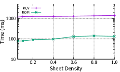
(b)

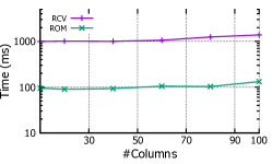
(c)

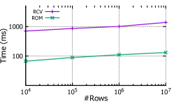
Figure 22: Update range performance vs (a) Sheet Density (b) Column Count (c) Row Count

(a)

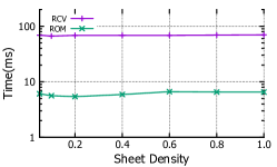
(b)

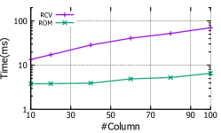
(c)

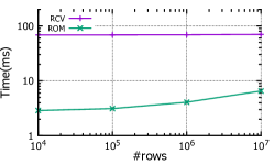
Figure 23: Insert row performance vs (a) Sheet Density (b) Column Count (c) Row Count

(a)

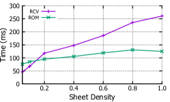
(b)

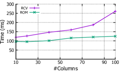
(c)

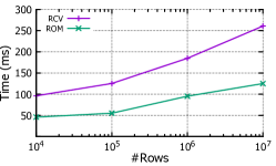
Figure 24: Select performance vs — (a) Sheet Density (b) Column Count (c) Row Count

Appendix C Additional Experiments

In this section, we present additional evaluation of the storage engine of DataSpread.

C-A Presentational Awareness and Access

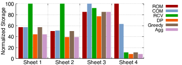
Figure 25: Storage comparison for sample spreadsheets.

C-A1 Drill-Down

We now drill deeper into the storage optimization algorithms and understand their behavior with respect to the characteristics of spreadsheets. We selected four sample sheets from our dataset to represent variations in terms of data density and layout of data, which is either horizontal for most part or vertical for most part. For these sheets, we contrast their storage requirements for the different data models. We plot the results in Figure 25, where we depict the normalized storage across sheets. For each sheet we have normalized the data model that performs the worst to $100$, and scaled the others accordingly.

The four spreadsheets show the variation among the different models in terms of storage requirements. Sheets 1 and 2 have substantial storage savings for ROM and COM when compared with RCV since they are relatively high density. On the other hand, Sheet 4 has has substantial storage savings for RCV as compared to ROM and COM due to its relatively low density. For Sheet 3 (4), ROM’s (COM’s) storage requirement is less then that of COM (ROM). This is due to the distribution of the cells, which span for the most part in the vertical direction for Sheet 3 and in the horizontal direction for Sheet 4. Except for Sheet 3, for all other sheets, the solution provided by Agg is close to DP. For Sheet 3, the optimization algorithms are not able to perform much better in terms of cost saving than the primitive data models. This is due to the fact that the sheet has both dense and sparse regions.

(a)

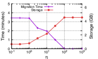
(b)

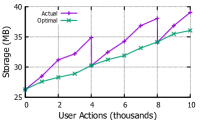
Figure 26: Incremental Hybrid Decomposition: (a) Trade-off with respect to $\eta$. (b) User operations vs. Storage.

C-A2 Incremental Maintenance

We now evaluate whether our representation schemes can be maintained efficiently in the face of edits. Note that in practice there will be periods where the DataSpread is idle, and so we can run the hybrid optimization algorithms then, but it is still valuable to ensure that the choice of data model is aware of the existing layout. To illustrate our incremental decomposition approach from Section A-C2, For this, we consider a synthetic spreadsheet as described in part e. of Section VII-B. We store the spreadsheet using the Agg-based hybrid data model. In the absence of user operation traces, we develop a generative model for update operations. We consider the following four operations. (i) Change the value of an existing cell. (ii) Add a new cell at an arbitrary location. (iii) Add a new row. (iv) Add a new column. Motivated from our user study, we consider that the above four operations are performed with probabilities $0.6$, $0.2$, $0.1999$, and $0.0001$ respectively. We fix the value of $\eta$ (the trade-off factor between migration and storage) to $1.0$ and run incremental maintenance with Agg after each batch of $1000$ user updates are performed. We plot the storage requirement against the number of user updates in Figure 26(b). The actual line in the graph indicates the storage requirement, which has a sawtooth like behavior. The drop in the graph correspond to the points where the incremental maintenance algorithm chose a new decomposition and migrated to it: thus, there was no migration performed at batch 1, 2, 3, but there was one at batch 4. We also plot the storage for the non-incremental variant of Agg, which we obtain by running incremental decomposition and setting $\eta$ to $0$. Overall, we find that a policy of this form (with $\eta=1$) only performs migration when the structure within the spreadsheet has substantially changed.

To study the impact of $\eta$, we consider one such point where the spreadsheet has diverged from its original Agg-based data model. We run the Agg variant of incremental maintenance algorithm on varying $\eta$. We plot $\eta$’s impact of the time taken to migrate and the storage requirement of the final decomposition in Figure 26(a). Here, as we increase the value of $\eta$ we observe that the migration time decreases and the storage requirement increases. At lower values of $\eta$, the algorithm gives preference to finding the optimal solution while ignoring the migration cost. We can observe this from the low storage cost, and the high time required to migrate the data in to the new decomposition. When $\eta>100$, the optimization aims at minimizing the migration cost at the expense of sacrificing the optimality of storage. Here, we observe a zero migration time, as the algorithm returns the original decomposition, and has the worst storage requirement.

C-B Presentational Access with Updates

C-B1 Varying Parameters

We now perform an evaluation of presentational access with updates on varying various parameters of the synthetic spreadsheets. For this evaluation, we focus on the two primitive data models i.e., ROM and RCV, with the spreadsheet being represented as a single table in these data models. Since we use synthetic datasets where cells are “filled in” with a certain probability, we did not involve hybrid data models, since they would (in this artificial context) typically end up preferring the ROM data model. These primitive data models are augmented with hierarchical positional mapping. We consider the performance on varying several parameters of these datasets: the density (i.e., the number of filled in cells), the number of rows, and the number of columns. The default values of these parameters are $1$, $10^{7}$ and $100$ respectively. We repeat each operation $500$ times and report the averages.

In Figure 24, we depict the charts corresponding to average time to perform a random select operation on a region of 1000 rows and 20 columns. This is, for example, the operation that would correspond to a user scrolling to a certain position on our spreadsheet. As can be seen in Figure 24(a), ROM starts dominating RCV beyond a certain density, at which point it makes more sense to store the data in as tuples that span rows instead of incurring the penalty of creating a tuple for every cell. Nevertheless, the best of these two models takes less than 150ms across sheets of varying densities. In Figure 24(b)(c), since the spreadsheet is very dense (density=1), ROM takes less time than RCV. Overall, in all cases, even on spreadsheets with 100 columns and $10^{7}$ rows and a density of 1, the average time to select a region is well within 500ms.

Figures 22 and 23 depict the corresponding charts for updating a region of 100 rows and 20 columns, and inserting one row of 100 columns for the primitive data models. In Figure 22, we find that the update time taken for RCV is a lot higher than the time for inserts or selects. This is because in this benchmark, DataSpread assumes that the entire region update happens at once, and fires $100\times 20=2000$ update queries one at a time. In practice, users may only update a small number of cells at a time; and further, we may be able to batch these queries or issue them in parallel to further save time. In Figure 23, we find that like in Figure 22, the time taken for updates on ROM is faster than RCV since it only needs to issue one query, while RCV needs to issue multiple queries. However, in this case, since the number of queries issued is small, the response time is always within $100$ms.

Overall, for both RCV and ROM, for inserting a row, the time is well below 500ms for all of the charts; for updates of a large region, while ROM is still highly interactive, RCV ends up taking longer since 1000s of queries need to be issued to the database. In practice, users won’t update such a large region at a time, and we can batch these queries.

Appendix D Primitive Data Models: Optimality Argument

Earlier in Section IV-B, we developed three primitive data models, that represent reasonable extremes if we are to represent and store a spreadsheet in a single table in a database system. Here, we argue that these models are optimal choices with respect to cascading updates, among a large class of data models that we shall describe now.

Requirements. We require each primitive data model in our class to have the following characteristics: (i) The data model should correspond to storing a rectangular region in the spreadsheet.This constraint naturally stems from the way we perceive tables in a two-dimensional interface, in the sense that tables are rectangular, and our data models are stored as rectangular tables on disk. (ii) The tuples in each table should correspond to a uniform geometric structure, and be contiguous in the sheet.The first part of the constraint arises because we store our tables in a relational database, necessitating all tuples to have the same number of attributes. Additionally, we want our tuples to correspond to contiguous regions in the spreadsheet, i.e., they should not have any “holes” in them.

Rectangular and Non-Rectangular Data Models. The data models which satisfy the aforementioned requirements fall into the following two classes: (i) Rectangular.In rectangular data models, each tuple corresponds to a rectangle in the sheet. Clearly, they are uniform geometric units, and are contiguous. A typical example is provided in Figure 27(a). (ii) Non-rectangular.Non-rectangular data models are essentially data-models where each tuple does not correspond to a rectangle. For instance, each tuple can either be diagonal with a fixed length, or have a “zig-zag” shape. A typical example where each tuple has zig-zag shape is provided in Figure 27(b).

(a)

(b)

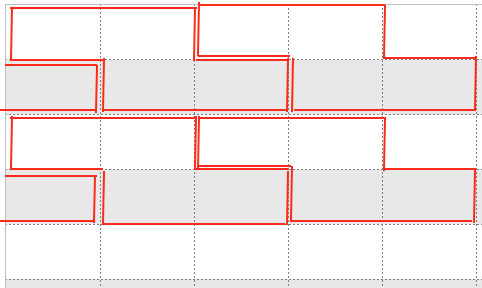
Figure 27: Data Model: (a) Rectangular (b) Non-rectangular

Updates as Optimality Criterion. We now discuss our optimality criterion. Since we consider a single table, storage is not a concern since every data model has to store all of the data in a table. Furthermore, with any vanilla index, e.g., B+ tree, access can be supported in all models in a similar manner, and likewise for single cells updates. Hence, we focus on updates on the sheet, and how they correspond to reorganizations in backend. Specifically, we focus on row/column inserts/deletes since changing values of existing data in the sheet would result in the same time complexity across all data models.

As we shall soon describe, row/column inserts/deletes can greatly influence the performance of our data models.

Theorem 10 (Optimality).

Our primitive data models, coupled with our hierarchical positional mapping schemes, are the only models which do not result in cascading updates from the class of data models discussed above.

Proof:

Consider any data model which can be rectangular or otherwise. We know all tuples are uniform in shape, and are contiguous in the sheet. Let say the tuple spans $p$ row and $q$ columns.

There are two possibilities: these tuples are either stored in row major form in the table or in column major form. If we use the former, then a row insert would result in data from $p$ rows to be shifted in the worst case. Equivalently, if the data is stored in column major form, then a column insert would result in data from $q$ columns to be shifted in the worst case. Therefore, cascading updates can be avoided only when one among $p$ and $q$ equals $1$. There are three cases now:

1. $p=1,q\neq 1$: This corresponds to ROM.

2. $p\neq 1,q=1$: This corresponds to COM.

3. $p=1,q=1$: This corresponds to RCV.

This completes our proof.∎

References

- [1] ZK Spreadsheet. https://www.zkoss.org/product/zkspreadsheet.
- [2] S. Abiteboul et al. The lowell database research self-assessment. Commun. ACM, 48(5):111–118, May 2005.
- [3] A. Abouzied et al. Dataplay: interactive tweaking and example-driven correction of graphical database queries. In UIST, 2012.
- [4] E. Bakke and E. Benson. The Schema-Independent Database UI: A Proposed Holy Grail and Some Suggestions. In CIDR, 2011.
- [5] E. Bakke et al. A spreadsheet-based user interface for managing plural relationships in structured data. In CHI, pages 2541–2550. ACM, 2011.
- [6] E. Bakke and D. R. Karger. Expressive query construction through direct manipulation of nested relational results. In SIGMOD. ACM, 2016.
- [7] M. Bendre, B. Sun, D. Zhang, X. Zhou, K. C.-C. Chang, and A. Parameswaran. Dataspread: Unifying databases and spreadsheets. VLDB Endowment, 8(12):2000–2003, Aug. 2015.
- [8] P. G. Brown. Overview of scidb: Large scale array storage, processing and analysis. In SIGMOD, pages 963–968. ACM, 2010.
- [9] S. P. Callahan et al. VisTrails: visualization meets data management. In SIGMOD, pages 745–747. ACM, 2006.
- [10] J. Callan, M. Hoy, C. Yoo, and L. Zhao. Clueweb09 data set, 2009.
- [11] T. Catarci, M. F. Costabile, S. Levialdi, and C. Batini. Visual query systems for databases: A survey. Journal of Visual Languages & Computing, 8(2):215–260, 1997.
- [12] U. Cetintemel et al. Query Steering for Interactive Data Exploration. In CIDR, 2013.
- [13] Z. Chen and M. Cafarella. Automatic web spreadsheet data extraction. In Proceedings of the 3rd International Workshop on Semantic Search Over the Web, pages 1:1–1:8. ACM, 2013.
- [14] Z. Chen, M. Cafarella, J. Chen, D. Prevo, and J. Zhuang. Senbazuru: A prototype spreadsheet database management system. VLDB, 6(12):1202–1205, 2013.
- [15] C. E. L. Cormen, Thomas H. and R. L. Rivest. Introduction to Algorithms. Cambridge. MA: MIT, 1990.
- [16] J. Culberson and R. Reckhow. Covering polygons is hard. Journal of Algorithms, 17(1):2 – 44, 1994.
- [17] J. Cunha, J. Saraiva, and J. Visser. From Spreadsheets to Relational Databases and Back. In SIGPLAN, PEPM ’09, pages 179–188, New York, NY, USA, 2009. ACM.
- [18] H. Gonzalez et al. Google fusion tables: web-centered data management and collaboration. In SIGMOD, pages 1061–1066. ACM, 2010.
- [19] S. Idreos and E. Liarou. dbtouch: Analytics at your fingertips. In CIDR, 2013.
- [20] H. V. Jagadish et al. Making database systems usable. In SIGMOD, pages 13–24. ACM, 2007.
- [21] N. Khoussainova et al. A Case for A Collaborative Query Management System. In CIDR. www.cidrdb.org, 2009.
- [22] N. Khoussainova et al. SnipSuggest: Context-aware autocompletion for SQL. VLDB Endowment, 4(1):22–33, 2010.
- [23] B. Klimt and Y. Yang. Introducing the enron corpus. In CEAS, 2004.
- [24] F. Li and H. Jagadish. Constructing an interactive natural language interface for relational databases. VLDB Endowment, 8(1), 2014.
- [25] A. Lingas, R. Y. Pinter, R. L. Rivest, and A. Shamir. Minimum edge length partitioning of rectilinear polygons. In Annual Allerton Conference on Communication, Control, and Computing, pages 53–63, 1982.
- [26] B. Liu and H. V. Jagadish. A spreadsheet algebra for a direct data manipulation query Interface. pages 417–428. IEEE, Mar. 2009.
- [27] J. Mackinlay, P. Hanrahan, and C. Stolte. Show me: Automatic presentation for visual analysis. TVCG, 13(6):1137–1144, 2007.
- [28] A. Nandi. Querying Without Keyboards. In CIDR, 2013.
- [29] A. Nandi and H. V. Jagadish. Guided interaction: Rethinking the query-result paradigm. VLDB Endowment, 4(12):1466–1469, 2011.
- [30] A. Nandi, L. Jiang, and M. Mandel. Gestural Query Specification. VLDB Endowment, 7(4), 2013.
- [31] L. Qian, K. LeFevre, and H. V. Jagadish. CRIUS: user-friendly database design. VLDB Endowment, 4(2):81–92, 2010.
- [32] V. Raman et al. Online dynamic reordering for interactive data processing. In VLDB, volume 99, pages 709–720, 1999.
- [33] V. Raman, B. Raman, and J. M. Hellerstein. Online dynamic reordering. The VLDB Journal, 9(3):247–260, Dec. 2000.
- [34] B. Shneiderman. Direct Manipulation: A Step Beyond Programming Languages. IEEE Computer, 16(8):57–69, 1983.
- [35] M. Singh, A. Nandi, and H. V. Jagadish. Skimmer: rapid scrolling of relational query results. In SIGMOD, pages 181–192. ACM, 2012.
- [36] C. Stolte et al. Polaris: A system for query, analysis, and visualization of multidimensional relational databases. TVCG, 8(1):52–65, 2002.
- [37] J. Tyszkiewicz. Spreadsheet as a relational database engine. In SIGMOD, pages 195–206. ACM, 2010.
- [38] http:/google.com/sheets. Google Sheets (retrieved March 10, 2015).
- [39] https://www.1010data.com/. 1010 Data (retrieved March 10, 2015).
- [40] https://www.airtable.com/. Airtable (retrieved March 10, 2015).
- [41] https://www.zoho.com/. Zoho Reports (retrieved March 10, 2015).
- [42] http://www.blockspring.com/. Blockspring (retrieved March 10, 2015).
- [43] http://www.excel-db.net/. Excel-DB (retrieved March 10, 2015).
- [44] http://www.microsoft.com/en-us/download/details.aspx?id=43348. Microsoft sql server power pivot (retrieved march 10, 2015).
- [45] C. Webb. Power Query for Power BI and Excel. Apress, 2014.
- [46] A. Witkowski et al. Advanced SQL modeling in RDBMS. ACM Transactions on Database Systems (TODS), 30(1):83–121, 2005.
- [47] A. Witkowski et al. Query by excel. In VLDB, pages 1204–1215. VLDB Endowment, 2005.
- [48] C. Yu and H. V. Jagadish. Schema summarization. In VLDB Endowment, pages 319–330, 2006.