Annealed scaling for a charged polymer in dimensions two and higher

Abstract.

This paper considers an undirected polymer chain on $\mathbb{Z}^{d}$, $d\geq 2$, with i.i.d. random charges attached to its constituent monomers. Each self-intersection of the polymer chain contributes an energy to the interaction Hamiltonian that is equal to the product of the charges of the two monomers that meet. The joint probability distribution for the polymer chain and the charges is given by the Gibbs distribution associated with the interaction Hamiltonian. The object of interest is the annealed free energy per monomer in the limit as the length $n$ of the polymer chain tends to infinity.

We show that there is a critical curve in the parameter plane spanned by the charge bias and the inverse temperature separating an extended phase from a collapsed phase. We derive the scaling of the critical curve for small and for large charge bias and the scaling of the annealed free energy for small inverse temperature. We show that in a subset of the collapsed phase the polymer chain is subdiffusive, namely, on scale $(n/\log n)^{1/(d+2)}$ it moves like a Brownian motion conditioned to stay inside a ball with a deterministic radius and a randomly shifted center. We expect this scaling to hold throughout the collapsed phase. We further expect that in the extended phase the polymer chain scales like a weakly self-avoiding walk.

The scaling of the critical curve for small charge bias and the scaling of the annealed free energy for small inverse temperature are both anomalous. Proofs are based on a detailed analysis for simple random walk of the downward large deviations of the self-intersection local time and the upward large deviations of the range. Part of our scaling results are rough. We formulate conjectures under which they can be sharpened. The existence of the free energy remains an open problem, which we are able to settle in a subset of the collapsed phase for a subclass of charge distributions.

1. Introduction and main results

In Caravenna, den Hollander, Pétrélis and Poisat [3], a detailed study was carried out of the annealed scaling properties of an undirected polymer chain on $\mathbb{Z}$ whose monomers carry i.i.d. random charges, in the limit as the length $n$ of the polymer chain tends to infinity. With the help of the Ray-Knight representation for the local times of simple random walk on $\mathbb{Z}$, a spectral representation for the annealed free energy per monomer was derived. This was used to prove that there is a critical curve in the parameter plane spanned by the charge bias and the inverse temperature, separating a ballistic phase from a subballistic phase. Various properties of the phase diagram were derived, including scaling properties of the critical curve for small and for large charge bias, and of the annealed free energy for small inverse temperature and near the critical curve. In addition, laws of large numbers, central limit theorems and large deviation principles were derived for the empirical speed and the empirical charge of the polymer chain in the limit as $n\to\infty$. The phase transition was found to be of first order, with the limiting speed and charge making a jump at the critical curve. The large deviation rate functions were found to have linear pieces, indicating the occurrence of mixed optimal strategies where part of the polymer is subballistic and the remaining part is ballistic.

The Ray-Knight representation is no longer available for $\mathbb{Z}^{d}$, $d\geq 2$. The goal of the present paper is to investigate what can be said with the help of other tools. In Section 1.1 we define the model, which was originally introduced in Kantor and Kardar [11]. In Section 1.2 we state our main theorems (Theorems 1.3, 1.5 and 1.6 below). In Section 1.3 we place these theorems in their proper context. In Section 1.4 we outline the remainder of the paper and list some open questions.

What makes the charged polymer model challenging is that the interaction is both attractive and repulsive. This places it outside the range of models that have been studied with the help of subadditivity techniques (see Ioffe [10] for an overview), and makes it into a testbed for the development of new approaches. The collapse transition of a charged polymer can be seen as a simplified version of the folding transition of a protein. Interactions between different parts of the protein cause it to fold into different configurations depending on the temperature.

Throughout the paper we use the notation $\mathbb{N}=\{1,2,\dots\}$ and $\mathbb{N}_{0}=\mathbb{N}\cup\{0\}$.

1.1. Model and assumptions

Let $S=(S_{i})_{i\in\mathbb{N}_{0}}$ be simple random walk on $\mathbb{Z}^{d}$, $d\geq 1$, starting at $S_{0}=0$. The path $S$ models the configuration of the polymer chain, i.e., $S_{i}$ is the location of monomer $i$. We use the letters $P$ and $E$ for probability and expectation with respect to $S$.

Let $\omega=(\omega_{i})_{i\in\mathbb{N}}$ be i.i.d. random variables taking values in $\mathbb{R}$. The sequence $\omega$ models the charges along the polymer chain, i.e., $\omega_{i}$ is the charge of monomer $i$ (see Fig. 1). We use the letters $\mathbb{P}$ and $\mathbb{E}$ for probability and expectation with respect to $\omega$, and assume that

(1.1) $$M(\delta)=\mathbb{E}[e^{\delta\omega_{1}}]<\infty\quad\forall\,\delta\in\mathbb{R}.$$

Without loss of generality (see (1.15) below) we further assume that

(1.2) $$\mathbb{E}[\omega_{1}]=0,\qquad\mathbb{E}[\omega_{1}^{2}]=1.$$

To allow for biased charges, we use the parameter $\delta$ to tilt $\mathbb{P}$, namely, we write $\mathbb{P}^{\delta}$ for the i.i.d. law of $\omega$ with marginal

(1.3) $$\mathbb{P}^{\delta}(\mathrm{d}\omega_{1})=\frac{e^{\delta\omega_{1}}\,\mathbb{P}(\mathrm{d}\omega_{1})}{M(\delta)}.$$

Without loss of generality we may take $\delta\in[0,\infty)$. Note that $\mathbb{E}^{\delta}[\omega_{1}]=M^{\prime}(\delta)/M(\delta)$.

Example 1.1.

If the charges are $+1$ with probability $p$ and $-1$ with probability $1-p$ for some $p\in(0,1)$, then $\mathbb{P}=[\tfrac{1}{2}(\delta_{-1}+\delta_{+1})]^{\otimes\mathbb{N}}$ and $\delta=\tfrac{1}{2}\log(\frac{p}{1-p})$. ∎

Let $\Pi$ denote the set of nearest-neighbour paths on $\mathbb{Z}^{d}$ starting at $0$. Given $n\in\mathbb{N}$, we associate with each $(\omega,S)\in\mathbb{R}^{\mathbb{N}}\times\Pi$ an energy given by the Hamiltonian (see Fig. 1)

(1.4) $$H_{n}^{\omega}(S)=\sum_{1\leq i<j\leq n}\omega_{i}\omega_{j}\,\mathbf{1}_{\{S_{i}=S_{j}\}}.$$

Let $\beta\in(0,\infty)$ denote the inverse temperature. Throughout the sequel the relevant space for the pair of parameters $(\delta,\beta)$ is the quadrant

(1.5) $$\mathcal{Q}=[0,\infty)\times(0,\infty).$$

Given $(\delta,\beta)\in\mathcal{Q}$, the annealed polymer measure of length $n$ is the Gibbs measure $\mathbb{P}_{n}^{\delta,\beta}$ defined as

(1.6) $$\frac{\mathrm{d}\mathbb{P}_{n}^{\delta,\beta}}{\mathrm{d}(\mathbb{P}^{\delta}\times P)}(\omega,S)=\frac{1}{\mathbb{Z}_{n}^{\delta,\beta}}\,e^{-\beta H_{n}^{\omega}(S)},\qquad(\omega,S)\in\mathbb{R}^{\mathbb{N}}\times\Pi,$$

where

(1.7) $$\mathbb{Z}_{n}^{\delta,\beta}=(\mathbb{E}^{\delta}\times E)\left[e^{-\beta H_{n}^{\omega}(S)}\right]$$

is the annealed partition function of length $n$. The measure $\mathbb{P}_{n}^{\delta,\beta}$ is the joint probability distribution for the polymer chain and the charges at charge bias $\delta$ and inverse temperature $\beta$, when the polymer chain has length $n$.

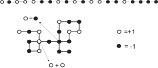
Figure 1. Top: A polymer chain of length $n=20$ carrying $(\pm 1)$-valued random charges. Bottom: The charges only interact at self-intersections: in the picture monomers $i=4,\,j=8$ meet and repel each other, while monomers $i=10,\,j=18$ meet and attract each other.

In what follows, instead of (1.4) we will work with the Hamiltonian

(1.8) $$H_{n}^{\omega}(S)=\sum_{1\leq i,j\leq n}\omega_{i}\omega_{j}\,\mathbf{1}_{\{S_{i}=S_{j}\}}=\sum_{x\in\mathbb{Z}^{d}}\left(\sum_{i=1}^{n}\omega_{i}\,\mathbf{1}_{\{S_{i}=x\}}\right)^{2}.$$

The sum under the square is the local time of $S$ at site $x$ weighted by the charges that are encountered in $\omega$. The change from (1.4) to (1.8) amounts to replacing $\beta$ by $2\beta$ (to add the terms with $i>j$) and changing the charge bias (to add the terms with $i=j$). The latter corresponds to tilting by $\delta\omega_{1}+\beta\omega_{1}^{2}$ instead of $\delta\omega_{1}$ in (1.3), which is the same as shifting $\delta$ by a value that depends on $\delta$ and $\beta$.

The expression in (1.7) can be rewritten as

(1.9) $$\mathbb{Z}_{n}^{\delta,\beta}=E\bigg{[}\prod_{x\in\mathbb{Z}^{d}}g_{\delta,\beta}\big{(}\ell_{n}(x)\big{)}\bigg{]},$$

where $\ell_{n}(x)=\sum_{i=1}^{n}\mathbf{1}_{\{S_{i}=x\}}$ is the local time at site $x$ up to time $n$, and

(1.10) $$g_{\delta,\beta}(\ell)=\mathbb{E}^{\delta}\big{[}\exp(-\beta\Omega_{\ell}^{2})\big{]},\qquad\Omega_{\ell}=\sum_{i=1}^{\ell}\omega_{i},\qquad\ell\in\mathbb{N}_{0}\,.$$

The annealed free energy per monomer is defined by

(1.11) $$F(\delta,\beta)=\limsup_{n\to\infty}\frac{1}{n}\log\mathbb{Z}_{n}^{\delta,\beta}.$$

Remark 1.2.

We expect, but are unable to prove, that the limes superior in (1.11) is a limit. A better name for $F$ would therefore be the pseudo annealed free energy per monomer, but we will not insist on terminology. Convergence appears to be hard to settle, due to the competition between attractive and repulsive interactions. Nonetheless, we are able to prove convergence for large enough $\beta$ and for charge distributions that are non-lattice with a bounded density (see Theorem 1.7 below). ∎

1.2. Main theorems

Our first theorem provides relevant upper and lower bounds on $F$. Abbreviate $f(\delta)=-\log M(\delta)\in(-\infty,0]$.

Theorem 1.3.

The limes superior in (1.11) takes values in $(-\infty,0]$ and satisfies the inequality $F(\delta,\beta)\geq f(\delta)$. ∎

The excess annealed free energy per monomer is defined by

(1.12) $$F^{*}(\delta,\beta)=F(\delta,\beta)-f(\delta).$$

It follows from (1.9)–(1.11) that

(1.13) $$F^{*}(\delta,\beta)=\limsup_{n\to\infty}\frac{1}{n}\log\mathbb{Z}_{n}^{*,\delta,\beta}$$

with

(1.14) $$\mathbb{Z}_{n}^{*,\delta,\beta}=E\bigg{[}\prod_{x\in\mathbb{Z}^{d}}g_{\delta,\beta}^{*}\big{(}\ell_{n}(x)\big{)}\bigg{]},$$

where

(1.15) $$g_{\delta,\beta}^{*}(\ell)=\mathbb{E}\big{[}\exp\big{(}\delta\Omega_{\ell}-\beta\Omega_{\ell}^{2}\big{)}\big{]},\qquad\ell\in\mathbb{N}_{0}.$$

(This expression shows why the assumption in (1.2) respresents no loss of generality.) We may think of $g_{\delta,\beta}^{*}(\ell)$ as a single-site partition function for a site that is visited $\ell$ times.

Example 1.4.

If the distribution of the charges is standard normal, then

(1.16) $$g_{\delta,\beta}^{*}(\ell)=\sqrt{\frac{1}{1+2\beta\ell}}\,\exp\left[\frac{\delta^{2}\ell}{2(1+2\beta\ell)}\right],\qquad\ell\in\mathbb{N}_{0}.$$

Note that $-\log g_{\delta,\beta}^{*}$ can be decomposed as $-\log g_{\delta,\beta}^{*}=-\log g^{*,\mathrm{att}}_{\delta,\beta}-\log g^{*,\mathrm{rep}}_{\delta,\beta}$ with

(1.17) $$-\log g^{*,\mathrm{att}}_{\delta,\beta}(\ell)=\frac{1}{2}\,\log(1+2\beta\ell),\qquad-\log g^{*,\mathrm{rep}}_{\delta,\beta}(\ell)=-\frac{\delta^{2}\ell}{2(1+2\beta\ell)}.$$

The former is an attractive interaction (positive concave function), the latter is a repulsive interaction (negative convex function). ∎

Because $F^{*}(\delta,\beta)\geq 0$, it is natural to define two phases:

(1.18) $$\mathcal{C} =\{(\delta,\beta)\in\mathcal{Q}\colon\,F^{*}(\delta,\beta)=0\},$$

$$\mathcal{E} =\{(\delta,\beta)\in\mathcal{Q}\colon\,F^{*}(\delta,\beta)>0\}.$$

For reasons that will become clear later, we refer to these as the collapsed phase, respectively, the extended phase. For every $\delta\in[0,\infty)$, $\beta\mapsto F^{*}(\delta,\beta)$ is finite, non-negative, non-increasing and convex. Hence there is a critical threshold $\beta_{c}(\delta)\in[0,\infty]$ such that $\mathcal{C}$ is the region on and above the curve and $\mathcal{E}$ is the region below the curve (see Fig. 2).

Figure 2. Qualitative plot of the critical curve $\delta\mapsto\beta_{c}(\delta)$ where the excess free energy $F^{*}(\delta,\beta)$ changes from being zero ($\mathcal{C}$) to being strictly positive ($\mathcal{E}$). The critical curve is part of $\mathcal{C}$.

Our second theorem describes the qualitative properties of the critical curve, provides scaling bounds for small charge bias, and identifies the asymptotics for large charge bias. Let

(1.19) $$Q_{n}=\sum_{x\in\mathbb{Z}^{d}}\ell_{n}(x)^{2}$$

denote the self-intersection local time at time $n$. A standard computation gives (see e.g. Spitzer [13, Section 7]), as $n\to\infty,$

(1.20) $$E[Q_{n}]=\sum_{1\leq i,j\leq n}P(S_{i}=S_{j})\sim\begin{cases}\lambda_{2}n\log n,&d=2,\\ \lambda_{d}n,&d\geq 3,\end{cases}$$

with

(1.21) $$\lambda_{2}=2/\pi,\qquad\lambda_{d}=2G_{d}-1,\quad d\geq 3,$$

where $G_{d}=\sum_{n\in\mathbb{N}_{0}}P(S_{n}=0)$ is the Green function at the origin of simple random walk on $\mathbb{Z}^{d}$. A similar computation yields (see Chen [4, Sections 5.4–5.5])

(1.22) $$\mathrm{Var}(Q_{n})=E[Q_{n}^{2}]-E[Q_{n}]^{2}\sim\begin{cases}C_{2}n^{2},&d=2,\\ C_{3}n\log n,&d=3,\\ C_{d}n,&d\geq 4,\end{cases}$$

with $C_{d}$, $d\geq 2$, computable constants. In particular, $Q_{n}$ satisfies the weak law of large numbers.

Abbreviate $m_{k}=\mathbb{E}[\omega_{1}^{k}]$, $k\in\mathbb{N}$, and recall that $m_{1}=0$, $m_{2}=1$ by (1.2).

Theorem 1.5.

(i) $\delta\mapsto\beta_{c}(\delta)$ is continuous, strictly increasing and convex on $[0,\infty)$, with $\beta_{c}(0)=0$.
(ii) As $\delta\downarrow 0$,

(1.23) $$\beta_{c}(\delta)=\tfrac{1}{2}\delta^{2}-\tfrac{1}{3}m_{3}\delta^{3}-\varepsilon_{\delta}$$

with

(1.24) $$[\underline{\kappa}+o(1)]\,\delta^{4}\leq\varepsilon_{\delta}\leq[1+o(1)]\begin{cases}\kappa_{2}\delta^{4}\log(1/\delta),&d=2,\\ \kappa_{d}\delta^{4},&d\geq 3,\end{cases}$$

where

(1.25) $$\underline{\kappa}=\tfrac{1}{12}m_{4}-\tfrac{1}{3}m_{3}^{2},\qquad\kappa_{d}=\begin{cases}\tfrac{1}{4}\lambda_{2},&d=2\\ \tfrac{1}{4}(\lambda_{d}-1)+\underline{\kappa},&d\geq 3.\end{cases}$$

(iii) As $\delta\to\infty$,

(1.26) $$\beta_{c}(\delta)\sim\frac{\delta}{T}$$

with

(1.27) $$T=\sup\big{\{}t>0\colon\,\mathbb{P}(\omega_{1}\in t\,\mathbb{Z})=1\big{\}}$$

(with the convention $\sup\emptyset=0$). Either $T>0$ (‘lattice case’) or $T=0$ (‘non-lattice case’). If $T=0$ and $\omega_{1}$ has a bounded density (with respect to the Lebesgue measure), then

(1.28) $$\beta_{c}(\delta)\sim\frac{\delta^{2}}{4\log\delta}.$$

∎

Our third theorem offers scaling bounds on the free energy for small inverse temperature and fixed charge bias.

Theorem 1.6.

For any $\delta\in(0,\infty)$, as $\beta\downarrow 0$,

(1.29) $$-\big{[}m(\delta)^{2}+v(\delta)+o(1)\big{]}\,\beta\geq F(\delta,\beta)\geq[1+o(1)]\left\{\begin{array}[]{ll}-\lambda_{2}m(\delta)^{2}\,\beta\log(1/\beta),&d=2,\\[5.69046pt] -\big{[}\lambda_{d}m(\delta)^{2}+v(\delta)\big{]}\,\beta,&d\geq 3,\end{array}\right.$$

where $m(\delta)=\mathbb{E}^{\delta}[\omega_{1}]$ and $v(\delta)={\mathbb{V}\mathrm{ar}}^{\delta}[\omega_{1}]$. ∎

Our fourth and last main theorem settles existence of the free energy for large enough inverse temperature for a subclass of charge distributions.

Theorem 1.7.

Suppose that the charge distribution is non-lattice $(T=0)$ and has a bounded density. Then there exists a curve $\delta\mapsto\beta_{0}(\delta)$ such that, for all $\beta\geq\beta_{0}(\delta)$,

1. the sequence $\{\log g^{*}_{\delta,\beta}(\ell)\}_{\ell\in\mathbb{N}}$ is super-additive,

2. the limes superior in (1.11) is a limit, and equals $-f(\delta)$,

3. the limes superior in (1.13) is a limit, and equals $0$.

Moreover, $\beta_{0}(\delta)\geq\beta_{c}(\delta)$ and $\beta_{0}(\delta)\sim\beta_{c}(\delta)$ as $\delta\to\infty$. ∎

1.3. Discussion and two conjectures

We discuss the theorems stated in Section 1.2 and place them in their proper context.

1. Theorem 1.3 shows that the annealed excess free energy $(\delta,\beta)\mapsto F^{*}(\delta,\beta)$ is nonnegative on $\mathcal{Q}$ and satisfies a lower bound that signals the presence of two phases.

2. Theorem 1.5(i) shows that there is a phase transition at a non-trivial critical curve $\delta\mapsto\beta_{c}(\delta)$ in $\mathcal{Q}$, separating a collapsed phase $\mathcal{C}$ (on and above the curve) from an extended phase $\mathcal{E}$ (below the curve). If the charge distribution is symmetric, then

(1.30) $$\beta_{c}(\delta)\leq\tfrac{1}{2}\delta^{2}\qquad\forall\,\delta\in[0,\infty).$$

Indeed, using (1.15) we may estimate

(1.31) $$g_{\delta,\tfrac{1}{2}\delta^{2}}^{*}(\ell) =\mathbb{E}\left[\exp\big{(}\delta\Omega_{\ell}-\tfrac{1}{2}\delta^{2}\Omega_{\ell}^{2}\big{)}\right]=\mathbb{E}\left[\sum_{k\in\mathbb{N}_{0}}\frac{1}{k!}(\delta\Omega_{\ell})^{k}\,\exp\big{(}-\tfrac{1}{2}\delta^{2}\Omega_{\ell}^{2}\big{)}\right]$$

$$=\mathbb{E}\left[\sum_{k\in\mathbb{N}_{0}}\frac{1}{(2k)!}(\delta\Omega_{\ell})^{2k}\,\exp\big{(}-\tfrac{1}{2}\delta^{2}\Omega_{\ell}^{2}\big{)}\right]$$

$$\leq\mathbb{E}\left[\sum_{k\in\mathbb{N}_{0}}\frac{1}{k!}(\tfrac{1}{2}\delta^{2}\Omega_{\ell}^{2})^{k}\,\exp\big{(}-\tfrac{1}{2}\delta^{2}\Omega_{\ell}^{2}\big{)}\right]=\mathbb{E}[1]=1\qquad\forall\,\ell\in\mathbb{N}_{0},$$

where we use that $(2k)!\geq 2^{k}\,k!$, $k\in\mathbb{N}_{0}$. Via (1.13)–(1.14) this implies that $\mathbb{Z}_{n}^{*,\delta,\tfrac{1}{2}\delta^{2}}\leq 1$ for all $n\in\mathbb{N}$ and hence $F^{*}(\delta,\tfrac{1}{2}\delta^{2})=0$, which via (1.18) yields (1.30) (see Fig. 2).

3. The lower and upper bounds in Theorem 1.5(ii) differ by a multiplicative factor when $d\geq 3$ and by a logarithmic factor when $d=2$. We expect that the upper bound gives the right asymptotic behaviour:

Conjecture 1.8.

As $\delta\downarrow 0$,

(1.32) $$\varepsilon_{\delta}\sim\begin{cases}\kappa_{2}\delta^{4}\log(1/\delta),&d=2,\\ \kappa_{d}\delta^{4},&d\geq 3.\end{cases}$$

∎

In Appendix C we state a conjecture about trimmed local times that would imply Conjecture 1.8. Theorem 1.5(ii) identifies three terms in the upper bound of $\beta_{c}(\delta)$ for small $\delta$, of which the last is anomalous for $d=2$. The proof is based on an analysis of the downward large deviations of the self-intersection local time $Q_{n}$ in (1.19) under the law $P$ of simple random walk in the limit as $n\to\infty$. A sharp result was found in Caravenna, den Hollander, Pétrélis and Poisat [3] for $d=1$, with two terms in the expansion of which the last is anomalous (namely, order $\delta^{8/3}$). For the standard normal distribution $m_{3}=0$ and $m_{4}=3$, and so $\kappa_{d}=\frac{1}{4}\lambda_{d}$ for $d\geq 2$ in (1.25).

4. Note that $\kappa_{d}\geq\underline{\kappa}>0$ for $d\geq 3$ when $m_{3}=0$, but not necessarily when $m_{3}\neq 0$. Indeed, if the distribution of the charges puts weight $\frac{1}{3N^{2}}$, $1-\tfrac{1}{2N^{2}}$, $\tfrac{1}{6N^{2}}$ on the values $-N$, $0$, $2N$, respectively, for some $N\in\mathbb{N}$, then $m_{1}=0$, $m_{2}=1$, $m_{3}=N$, $m_{4}=3N^{2}$, in which case $-\tfrac{1}{3}m_{3}^{2}+\tfrac{1}{12}m_{4}=-\tfrac{1}{12}N^{2}$. This gives $\kappa_{d}<0$ for $N$ large enough and $\underline{\kappa}<0\leq\kappa_{d}$ for $N$ small enough.

5. Theorem 1.5(iii) identifies the asymptotics of $\beta_{c}(\delta)$ for large $\delta$, which is the same as for $d=1$. The scaling depends on whether the charge distribution is lattice or non-lattice.

6. In analogy with what we saw in Theorem 1.5(ii), the bounds in Theorem 1.6 do not match, but we expect the following:

Conjecture 1.9.

For any $\delta\in(0,\infty)$, as $\beta\downarrow 0$,

(1.33) $$F(\delta,\beta)\sim\left\{\begin{array}[]{ll}-\lambda_{2}m(\delta)^{2}\,\beta\log(1/\beta),&d=2,\\[5.69046pt] -\big{[}\lambda_{d}m(\delta)^{2}+v(\delta)\big{]}\,\beta,&d\geq 3,\end{array}\right.$$

∎

This identifies the scaling behaviour of the free energy for small inverse temperature (i.e., in the limit of weak interaction). The scaling is anomalous for $d=2$, as it was in [3] for $d=1$ (namely, order $\beta^{2/3}$).

7. Theorem 1.7 settles the existence of the free energy in a subset of the collapsed phase for a subclass of charge distributions. The limit is expected to exist always.

8. As shown in den Hollander [9, Chapter 8], for every $d\geq 1$ and every $(\delta,\beta)\in\mathrm{int}(\mathcal{C})$,

(1.34) $$\lim_{n\to\infty}\frac{(\alpha_{n})^{2}}{n}\,\log\mathbb{Z}_{n}^{*,\delta,\beta}=-\chi_{d},$$

with $\alpha_{n}=(n/\log n)^{1/(d+2)}$ and with $\chi_{d}\in(0,\infty)$ a constant that is explicitly computable. The idea behind (1.34) is that the empirical charge makes a large deviation under the law $\mathbb{P}^{\delta}$ so that it becomes zero. The price for this large deviation is

(1.35) $$e^{-nH(\mathbb{P}^{0}\,|\,\mathbb{P}^{\delta})+o(n)},\qquad n\to\infty,$$

where $H(\mathbb{P}^{0}\,|\,\mathbb{P}^{\delta})$ denotes the specific relative entropy of $\mathbb{P}^{0}=\mathbb{P}$ with respect to $\mathbb{P}^{\delta}$. Since the latter equals $\log M(\delta)=-f(\delta)$, this accounts for the term that is subtracted in the excess free energy. Conditional on the empirical charge being zero, the attraction between charged monomers with the same sign wins from the repulsion between charged monomers with opposite sign, making the polymer chain contract to a subdiffusive scale $\alpha_{n}$. This accounts for the correction term in the free energy. It is shown in [9] that, under the law $\mathbb{P}^{\delta}$,

(1.36) $$\left(\frac{1}{\alpha_{n}}\,S_{\lfloor nt\rfloor}\right)_{0\leq t\leq 1}\Longrightarrow(U_{t})_{0\leq t\leq 1},\qquad n\to\infty,$$

where $\Longrightarrow$ denotes convergence in distribution and $(U_{t})_{t\geq 0}$ is a Brownian motion on $\mathbb{R}^{d}$ conditioned not to leave a ball with a deterministic radius and a randomly shifted center (see Fig. 3). Compactification is a key step in the sketch of the proof provided in den Hollander [9, Chapter 8], which requires super-additivity of $\{\log g^{*}_{\delta,\beta}(\ell)\}_{\ell\in\mathbb{N}}$. From Theorem 1.7(1) we know that this property holds at least for $\beta$ large enough.

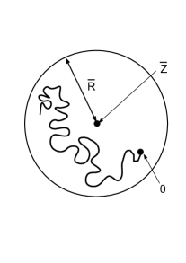
Figure 3. A Brownian motion starting at $0$ conditioned to stay inside the ball with radius $\bar{R}$ and center $\bar{Z}$. Formulas for $\bar{R}$ and the distribution of $\bar{Z}$, concentrated on the ball of radius $\bar{R}$ centered at $0$, are given in [9, Chapter 8].

9. It is natural to expect that for every $(\delta,\beta)\in\mathcal{E}$ the polymer behaves like weakly self-avoiding walk. Once the empirical charge is strictly positive, the repulsion should win from the attraction, and the polymer should scale as if all the charges were strictly positive, with a change of time scale only.

10. Brydges, van der Hofstad and König [1] derive a formula for the joint density of the local times of a continuous-time Markov chain on a finite graph, using tools from finite-dimensional complex calculus. This representation, which is the analogue of the Ray-Knight representation for the local times of one-dimensional simple random walk, involves a large determinant and therefore appears to be intractable for the analysis of the annealed charged polymer.

1.4. Outline and open questions

The remainder of this paper is organised as follows. In Section 2 we study the downward large deviations of the self-intersection local time $Q_{n}$ defined in (1.19) under the law $P$ of simple random walk. We derive the qualitative properties of the rate function, which amounts to controlling the partition function (and free energy) of weakly self-avoiding walk with the help of cutting arguments. In Section 3 we prove Theorem 1.3. In Section 4 we prove Theorem 1.5. The proof of part (i) requires a detailed analysis of the function $\ell\mapsto g_{\delta,\beta}^{*}(\ell)$ defined in (1.15). The proof of part (ii) is based on estimates of the function $\ell\mapsto g_{\delta,\beta}^{*}(\ell)$ for small values of $\delta$. The proof of part (iii) carries over from [3]. In Section 5 we use the results in Section 2 to prove Theorem 1.6, and in Section 6 we prove Theorem 1.7. In Appendix A we collect some estimates on simple random walk constrained to be a bridge, which are needed along the way. In Appendix B we state a conjecture on weakly self-avoiding walk that complement the results in Section 2. In Appendix C we discuss a rough estimate on the probability of an upward large deviation for the range of simple random walk, trimmed when the local times exceed a given threshold. This estimate appears to be the key to Conjectures 1.8 and 1.9.

Here are some open questions:

• Is the limes superior in (1.11) always a limit? For $d=1$ the answer was found to be yes.

• Is $(\delta,\beta)\mapsto F^{*}(\delta,\beta)$ analytic throughout the extended phase $\mathcal{E}$? For $d=1$ the answer was found to be yes.

• How does $F^{*}(\delta,\beta)$ behave as $\beta\uparrow\beta_{c}(\delta)$? Is the phase transition first order, as for $d=1$, or higher order?

• Is the excess free energy monotone in the dimension, i.e., $F^{*\,(d+1)}(\delta,\beta)\geq F^{*\,(d)}(\delta,\beta)$ for all $(\delta,\beta)\in\mathcal{Q}$ and $d\geq 1$?

• What is the nature of the expansion of $\beta_{c}(\delta)$ for $\delta\downarrow 0$, of which (1.23) gives the first three terms? Is it anomalous with a logarithmic correction to the term of order $\delta^{2d}$ for any $d\geq 3$?

2. Weakly self-avoiding walk

In Section 2.1 we look at the free energy $f^{\mathrm{wsaw}}$ of the weakly self-avoiding walk, identify its scaling in the limit of weak interaction (Proposition 2.2 below). In Section 2.2 we look at the rate function for the downward large deviations of the self-intersection local time $Q_{n}$ as $n\to\infty$ (Proposition 2.3 below). In Section 2.3 we use this rate function to prove the scaling of $f^{\mathrm{wsaw}}$.

Remark 2.1.

Let $\mathcal{B}_{n}$ be the set of $n$-step bridges

(2.1) $$\mathcal{B}_{n}=\left\{S\in\Pi\colon\,0=S^{(1)}_{0}<S^{(1)}_{i}<S^{(1)}_{n}\,\,\forall\,0<i<n\right\},$$

where $S^{(1)}$ stands for the first coordinate of simple random walk $S$. At several points in the paper we will use that there exists a $C\in(0,\infty)$ such that

(2.2) $$\lim_{n\to\infty}n\,P(S\in\mathcal{B}_{n})=C,$$

a property we will prove in Appendix A.1. ∎

2.1. Self-intersection local time

Recall the definition of the self-intersection local time $Q_{n}=\sum_{x\in\mathbb{Z}^{d}}\ell_{n}(x)^{2}$ in (1.19). For $u\geq 0$, let

(2.3) $$Z_{n}^{\mathrm{wsaw}}(u)=E\big{[}e^{-uQ_{n}}\big{]},\qquad u\in[0,\infty),$$

be the partition function of weakly self-avoiding walk. This quantity is submultiplicative because $Q_{n+m}\geq Q_{n}+Q_{m}$, $m,n\in\mathbb{N}$. Hence (minus) the free energy of the weakly self-avoiding walk

(2.4) $$f^{\mathrm{wsaw}}(u)=-\lim_{n\to\infty}\frac{1}{n}\log Z_{n}^{\mathrm{wsaw}}(u),\qquad u\in[0,\infty),$$

exists. The following lemma identifies the scaling behaviour of $f^{\mathrm{wsaw}}(u)$ for $u\downarrow 0$.

Proposition 2.2.

As $u\downarrow 0$

(2.5) $$f^{\mathrm{wsaw}}(u)\sim\begin{cases}\lambda_{1}u^{1/3},&d=1,\\ \lambda_{2}u\log(1/u),&d=2,\\ \lambda_{d}u,&d\geq 3,\end{cases}$$

where $\lambda_{d}$ is given in (1.21). ∎

Proposition 2.2 extends the downward moderate deviation result for $Q_{n}$ derived by Chen [4, Theorem 8.3.2]. For more background on large deviation theory, see den Hollander [8]. We comment further on this result in Appendix B, where we discuss the rate of convergence to $f^{\mathrm{wsaw}}(u)$ and the higher order terms in the asymptotic expansion of $f^{\mathrm{wsaw}}(u)$ as $u\downarrow 0$.

2.2. Downward large deviations of the self-intersection local time

In Section 2.3 we will show that Proposition 2.2 is a consequence of the following lemma describing the downward large deviation behaviour of $Q_{n}$ (see Fig. 4).

Proposition 2.3.

The limit

(2.6) $$I(t)=\lim_{n\to\infty}\left[-\frac{1}{n}\log P(Q_{n}\leq tn)\right],\qquad t\in[1,\infty),$$

exists. Moreover, $t\mapsto I(t)$ is finite, non-negative, non-increasing and convex on $[1,\infty)$, and satisfies

(2.7) $$d=2\colon\quad I(t)>0,\quad t\geq 1,\qquad d\geq 3\colon\quad I(t)\left\{\begin{array}[]{ll}>0,&1\leq t\leq\lambda_{d},\\ =0,&t\geq\lambda_{d}.\end{array}\right.$$

Furthermore,

(2.8) $$d=2\colon\quad\lim_{t\to\infty}\frac{-\log I(t)}{t}=\frac{1}{\lambda_{2}}.$$

∎

Figure 4. Qualitative plots of $t\mapsto I(t)$ for $d=2$ and $d\geq 3$.

Proof.

The proof comes in 5 Steps. Steps 1–2 use bridges and superadditivity, Steps 3–5 use cutting arguments.

1. Existence, finiteness and monotonicity of $I$. Recall (2.1). Let $\mathcal{B}_{n}$ be short for $\{S\in\mathcal{B}_{n}\}$. Define

(2.9) $$u(n)=P(Q_{n}\leq tn,\,\mathcal{B}_{n}),\quad n\in\mathbb{N}.$$

The sequence $(\log u(n))_{n\in\mathbb{N}}$ is superadditive. Therefore $\lim_{n\to\infty}[-\frac{1}{n}\log u(n)]=\bar{I}(t)\in[0,\infty]$ exists. Clearly,

(2.10) $$\limsup_{n\to\infty}\left[-\frac{1}{n}\log P(Q_{n}\leq tn)\right]\leq\bar{I}(t).$$

The reverse inequality follows from a standard unfolding procedure applied to bridges that decreases $Q_{n}$. Indeed, using the bound introduced in Hammersley and Welsh [7], we get

(2.11) $$|\{Q_{n}\leq tn\}|\leq e^{\pi\sqrt{\frac{n}{3}}(1+o(1))}|\{Q_{n}\leq tn\}\cap\mathcal{B}_{n}|,$$

from which it follows that

(2.12) $$\liminf_{n\to\infty}\left[-\frac{1}{n}\log P(Q_{n}\leq tn)\right]\geq\bar{I}(t).$$

Combining (2.10) and (2.12), we get (2.6) with $I=\bar{I}$. Finally, it is obvious that $t\mapsto I(t)$ is non-increasing on $[1,\infty)$. Since $\{Q_{n}=n\}=\{(S_{i})_{i=0}^{n}\text{ is self-avoiding}\}$, we have $I(1)=\log\mu_{c}(\mathbb{Z}^{d})<\infty$, with $\mu_{c}(\mathbb{Z}^{d})$ the connective constant of $\mathbb{Z}^{d}$.

2. Convexity of $I$. Every $2n$-step walk $S_{[0,2n]}=(S_{i})_{0\leq i\leq 2n}$ can be decomposed into two $n$-step walks: $S_{[0,n]}=(S_{i})_{0\leq i\leq n}$ and $\bar{S}_{[0,n]}=(S_{n+i}-S_{n})_{0\leq i\leq n}$. Fix $a,b>0$. Restricting both parts to be a bridge, we get

(2.13) $$P(Q_{2n}\leq(a+b)n,\,\mathcal{B}_{2n}) \geq P\Big{(}Q_{n}\leq an,\,\bar{Q}_{n}\leq bn,\,S\in\mathcal{B}_{n}\,,\bar{S}\in\mathcal{B}_{n}\Big{)}$$

$$=P\big{(}Q_{n}\leq an,\,S\in\mathcal{B}_{n}\big{)}\,P\big{(}Q_{n}\leq bn,\,S\in\mathcal{B}_{n}\big{)},$$

where $\bar{Q}_{n}=\sum_{1\leq i,j\leq n}\mathbf{1}_{\{\bar{S}_{i}=\bar{S}_{j}\}}$. Taking the logarithm, diving by $2n$ and letting $n\to\infty$, we get

(2.14) $$I\left(\tfrac{1}{2}(a+b)\right)\leq\tfrac{1}{2}[I(a)+I(b)].$$

3. Two regimes of $I$ for $d\geq 3$. Clearly, $I(t)=0$ for $t\geq\lambda_{d}$. To prove that $I(t)>0$ for $1\leq t<\lambda_{d}$, we cut $[0,n]$ into sub-intervals of length $1/\eta$, where $\eta>0$ is small and $\eta n$ is integer. Note that

(2.15) $$Q_{n}\geq\sum_{1\leq k\leq\eta n}Q^{(k)},\qquad Q^{(k)}=\sum_{\frac{k-1}{\eta}+1\leq i,j\leq\frac{k}{\eta}}\mathbf{1}_{\{S_{i}=S_{j}\}}.$$

Fix $\varepsilon>0$ small. Then, by (1.20), there exists an $\eta_{\varepsilon}$ such that $E[Q^{(1)}]\geq\frac{1}{\eta}(\lambda_{d}-\varepsilon^{2})$ for $0<\eta\leq\eta_{\varepsilon}$. Moreover, by the Markov property of simple random walk, the $Q^{(k)}$’s are independent. Therefore we may estimate, for $\gamma>0$,

(2.16) $$P\big{(}Q_{n}\leq(\lambda_{d}-\varepsilon)n\big{)}\leq P\left(-\gamma\sum_{1\leq k\leq\eta n}Q^{(k)}\geq-\gamma(\lambda_{d}-\varepsilon)n\right)$$

$$\qquad\leq e^{\gamma(\lambda_{d}-\varepsilon)n}E\big{[}e^{-\gamma Q^{(1)}}\big{]}^{\eta n}\leq e^{\gamma(\lambda_{d}-\varepsilon)n}\Big{(}1-\gamma E[Q^{(1)}]+\tfrac{1}{2}\gamma^{2}E[(Q^{(1)})^{2}]\Big{)}^{\eta n}$$

$$\qquad\leq e^{\gamma(\lambda_{d}-\varepsilon)n}\,e^{\big{(}-\gamma E[Q^{(1)}]+\tfrac{1}{2}\gamma^{2}E[(Q^{(1)})^{2}]\big{)}\,\eta n}\leq e^{-n\gamma\big{(}\varepsilon-\tfrac{1}{2}\eta\gamma E[(Q^{(1)})^{2}]\big{)}}.$$

Because $Q^{(1)}\leq 1/\eta^{2}$ (and hence $E[(Q^{(1)})^{2}]\leq 1/\eta^{4}$), it suffices to choose $\gamma$ small enough to get from (2.6) that $I(\lambda_{d}-\varepsilon)>0$. Since $\varepsilon>0$ is arbitrary, this proves the claim.

4. Positivity and asymptotics of $I$ for $d=2$. To obtain a lower bound on the probability $P(Q_{n}\leq tn)$ we use a specific strategy, explained informally in Fig. 5. Let $\varepsilon>0$ and

(2.17) $$m=\lfloor e^{\frac{t}{(1+\varepsilon)\lambda_{2}}}\rfloor\geq 2.$$

Figure 5. Informal description of the specific strategy to obtain $Q_{n}\leq tn$: Confine $(S_{i})_{i=0}^{n}$ to $n/m$ consecutive strips, each containing $m\approx e^{t/\lambda_{2}}$ steps. On each strip impose the walk to be a bridge. By (1.20), each strip contributes $\lesssim\lambda_{2}m\log m$ to the self-intersection local time, and hence $Q_{n}\lesssim\frac{n}{m}(\lambda_{2}m\log m)\approx tn$. The cost per bridge is $\approx 1/m$. Consequently, the cost of the consecutive strip strategy is $(1/m)^{n/m}\approx\exp(-nm^{-1}\log m)$. Hence $I(t)\lesssim m^{-1}\log m=c\,te^{-t/\lambda_{2}}$.

For $n\in\mathbb{N}$, write $n=pm+q$, where $p=p(n)\in\mathbb{N}_{0}$ and $0<q=q(n)\leq m$. For $k\in\mathbb{N}$, define the events

(2.18) $$U_{k} =\Big{\{}S^{(1)}_{(k-1)m}\leq S^{(1)}_{i}\leq S^{(1)}_{km-1}\,\,\forall\,(k-1)m<i<km,\,S^{(1)}_{km}=S^{(1)}_{km-1}+1\Big{\}},$$

$$V_{k} =\{Q^{(k)}\leq(1+\varepsilon)\lambda_{2}m\log m\},$$

with $Q^{(k)}$ as in (2.15) with $1/\eta=m$, and

(2.19) $$W=\left[\bigcap_{k=1}^{p}U_{k}\cap V_{k}\right]\bigcap\left[\bigcap_{j=1}^{q}\left\{S^{(1)}_{pm+j}=S^{(1)}_{pm}+j\right\}\right].$$

Note that, on the event $W$,

(2.20) $$Q_{n}=\sum_{k=1}^{p}Q^{(k)}\leq(1+\varepsilon)\lambda_{2}\,p\,m\log m\leq tn.$$

Hence

(2.21) $$P(Q_{n}\leq tn)\geq P(Q_{n}\leq tn,\,W)\geq\Big{[}\frac{1}{4}\,P\big{(}Q_{m}\leq(1+\varepsilon)\lambda_{2}m\log m,\,S\in\mathcal{B}_{m}\big{)}\Big{]}^{p}\Big{(}\frac{1}{4}\Big{)}^{q}.$$

We therefore obtain

(2.22) $$\frac{1}{n}\log P(Q_{n}\leq tn)\geq\frac{1-\frac{q}{n}}{m}\Big{[}\log P\big{(}Q_{m}\leq(1+\varepsilon)\lambda_{2}m\log m,\,S\in\mathcal{B}_{m}\big{)}-\log 4\Big{]}-\frac{q}{n}\log 4$$

and, by taking the limit $n\to\infty$, we get

(2.23) $$\liminf_{n\to\infty}\frac{1}{n}\log P(Q_{n}\leq tn)\geq\frac{1}{m}\Big{[}\log P\big{(}Q_{m}\leq(1+\varepsilon)\lambda_{2}m\log m,\,S\in\mathcal{B}_{m}\big{)}-\log 4\Big{]}.$$

In Appendix A.2 we prove that

(2.24) $$P\big{(}Q_{m}\leq(1+\varepsilon)\lambda_{2}m\log m,\,S\in\mathcal{B}_{m}\big{)}\sim P(S\in\mathcal{B}_{m}),\qquad m\to\infty.$$

Therefore, by (2.2), the right-hand side of (2.23) scales like $-\log m/m$ as $m\to\infty$. Combining (2.6), (2.17) and (2.23)–(2.24), we arrive at

(2.25) $$I(t)\leq\frac{t}{(1+\varepsilon)\lambda_{2}}\,e^{-\frac{t}{(1+\varepsilon)\lambda_{2}}}[1+o(1)],\qquad t\to\infty.$$

This proves that $\liminf_{t\to\infty}-\log I(t)/t\geq 1/(1+\varepsilon)\lambda_{2}$. Let $\varepsilon\downarrow 0$ to get the lower half of (2.8).

5. To obtain an upper bound on the probability $P(Q_{n}\leq tn)$ we use the same type of strategy. Let $\varepsilon>0$, choose $m$ large enough so that $E[Q^{(1)}]\geq(1-\varepsilon)\lambda_{2}m\log m$, and use that there exists a constant $c$ such that $E[Q_{n}^{2}]\leq c(n\log n)^{2}$. Cut $[0,n]$ into sub-intervals of length $m$, similarly as in (2.15) with $m$ instead of $1/\eta$ (assume that $n/m$ is integer). Estimate

$$P(Q_{n}\leq tn) \leq P\Big{(}\sum_{1\leq i\leq n/m}Q^{(i)}\leq tn\Big{)}\leq e^{\gamma tn}E\big{[}e^{-\gamma Q^{(1)}}\big{]}^{n/m}$$

(2.26) $$\leq e^{\gamma tn}e^{\frac{n}{m}\big{(}-\gamma E[Q^{(1)}]+\tfrac{1}{2}\gamma^{2}E[(Q^{(1)})^{2}]\big{)}}\leq e^{\gamma tn}e^{\frac{n}{m}\big{(}-\gamma(1-\varepsilon)\lambda_{2}m\log m+c\tfrac{1}{2}\gamma^{2}m^{2}(\log m)^{2}\big{)}}.$$

Choose $m=\lfloor e^{\frac{1+\varepsilon}{1-\varepsilon}\frac{t}{\lambda_{2}}}\rfloor$, which diverges as $t\to\infty$. Then (2.2) becomes

(2.27) $$P(Q_{n}\leq tn)\leq e^{-n\gamma\big{(}-t\varepsilon+c\tfrac{1}{2}\gamma m(\log m)^{2}\big{)}}.$$

Optimizing over $\gamma$, i.e., choosing $\gamma=t\varepsilon/c\,m(\log m)^{2}$, we get

(2.28) $$P(Q_{n}\leq tn)\leq\exp\Big{(}-c(\varepsilon)e^{-\frac{1+\varepsilon}{1-\varepsilon}\frac{t}{\lambda_{2}}}n\Big{)}$$

for some constant $c(\varepsilon)>0$, and so we arrive at

(2.29) $$I(t)\geq c(\varepsilon)\,e^{-\frac{1+\varepsilon}{1-\varepsilon}\frac{t}{\lambda_{2}}},\qquad t\to\infty.$$

This proves that $\limsup_{t\to\infty}-\log I(t)/t\leq(1+\varepsilon)/(1-\varepsilon)\lambda_{2}$. Let $\varepsilon\downarrow 0$ to get the upper half of (2.8), which completes the proof of Proposition 2.3. ∎

Remark 2.4.

We may adapt the argument in Step 4 to obtain a result that will be needed in (4.37) below, namely, a lower bound on the probability

(2.30) $$v_{n}(t)=P\left(Q_{n}\leq tn,\,\max_{x\in\mathbb{Z}^{2}}\ell_{n}(x)\leq c_{1}e^{c_{2}t}\right)$$

with $c_{1}>0$, $c_{2}=\big{(}2\lambda_{2}(1+\tfrac{1}{4}\varepsilon)\big{)}^{-1}$ and $\varepsilon>0$ small. This lower bound reads

(2.31) $$\liminf_{n\to\infty}\frac{1}{n}\log v_{n}(t)\geq-\frac{t}{(1+\varepsilon)\lambda_{2}}\,e^{-\frac{t}{(1+\varepsilon)\lambda_{2}}}[1+o(1)],\qquad t\to\infty.$$

Indeed, the strategy above is still valid, and (2.23) becomes

(2.32) $$\liminf_{n\to\infty}\frac{1}{n}\log v_{n}(t)$$

$$\qquad\geq\frac{1}{m}\Big{[}\log P\Big{(}Q_{m}\leq(1+\varepsilon)\lambda_{2}m\log m,\,\max_{x\in\mathbb{Z}^{2}}\ell_{m}(x)\leq c_{1}m^{c_{3}},\,S\in\mathcal{B}_{m}\Big{)}-\log 4\Big{]}$$

with $m$ as in (2.17) and $c_{3}=\tfrac{1}{2}(1+\varepsilon)/(1+\tfrac{1}{4}\varepsilon)$. Since the local times are typically of order $\log m$, the constraint on the maximum of the local times is harmless in the limit as $m\to\infty$ and can be removed. After that we obtain (2.31) following the argument in (2.23)–(2.24). To check that the constraint can be removed, estimate

(2.33) $$P\Big{(}\max_{x\in\mathbb{Z}^{2}}\ell_{m}(x)>c_{1}m^{c_{3}}\Big{)}\leq mP\big{(}\ell_{m}(0)>c_{1}m^{c_{3}}\big{)}$$

$$\qquad\leq m\left(1-\frac{c_{4}}{\log m}\right)^{c_{1}m^{c_{3}}}\leq m\,e^{-c_{1}c_{4}m^{c_{3}}\log m},$$

which is $o(1/m)$. ∎

2.3. Scaling of the free energy of weakly self-avoiding walk

In this section we prove Proposition 2.2.

Proof.

From Proposition 2.3 and Varadhan’s lemma we obtain

(2.34) $$-f^{\mathrm{wsaw}}(u)=\sup_{t\in[1,\infty)}[-tu-I(t)].$$

Upper bound: For $d\geq 3$, choose $t=\lambda_{d}$ and use that $I(\lambda_{d})=0$, to obtain $-f^{\mathrm{wsaw}}(u)\geq-\lambda_{d}u$ for all $u$, which is the upper half of (2.5).

For $d=2$, by (2.8), for any $\varepsilon>0$ we have $I(t)\leq e^{-(1-\varepsilon)t/\lambda_{2}}$ for $t$ large enough. Choose $t=(1-\varepsilon)^{-1}\lambda_{2}\log(1/u)$ to obtain $-f^{\mathrm{wsaw}}(u)\geq-(1-\varepsilon)^{-1}\lambda_{2}u\log(1/u)-u$, so that

(2.35) $$\limsup_{u\downarrow 0}\frac{f^{\mathrm{wsaw}}(u)}{u\log(1/u)}\leq(1-\varepsilon)^{-1}\lambda_{2}.$$

Let $\varepsilon\downarrow 0$ to get the upper half of (2.5).

Lower bound: For $d\geq 3$, write

(2.36) $$-f^{\mathrm{wsaw}}(u)=\sup_{1\leq t\leq\lambda_{d}}[-tu-I(t)]=-\lambda_{d}u+\sup_{1\leq t\leq\lambda_{d}}[(\lambda_{d}-t)u-I(t)].$$

Fix $\varepsilon>0$ small. Then $I(\lambda_{d}-\varepsilon)>0$. By convexity, $I(t)\geq\frac{\lambda_{d}-t}{\varepsilon}I(\lambda_{d}-\varepsilon)$ for all $1\leq t\leq\lambda_{d}-\varepsilon$. Therefore

(2.37) $$-f^{\mathrm{wsaw}}(u)\leq-\lambda_{d}u+\sup_{1\leq t\leq\lambda_{d}-\varepsilon}\left[(\lambda_{d}-t)u-\tfrac{\lambda_{d}-t}{\varepsilon}I(\lambda_{d}-\varepsilon)\right]\vee\sup_{\lambda_{d}-\varepsilon<t\leq\lambda_{d}}[(\lambda_{d}-t)u-I(t)].$$

For $u\leq I(\lambda_{d}-\varepsilon)/\varepsilon$ the first supremum is non-positive and the second supremum is at most $\varepsilon u$. This implies that $f^{\mathrm{wsaw}}(u)\geq(\lambda_{d}-\varepsilon)u$ for $u$ small enough (namely, $u\leq I(\lambda_{d}-\varepsilon)/\varepsilon$). Let $\varepsilon\downarrow 0$ to get the lower half of (2.5).

For $d=2$, by (2.8), for any $\varepsilon>0$ we have $I(t)\geq e^{-(1+\varepsilon)t/\lambda_{2}}$ for $t$ large enough. We have

(2.38) $$-f^{\mathrm{wsaw}}(u) \leq\sup_{1\leq t\leq t_{0}}[-tu-I(t)]\ \vee\,\sup_{t\geq t_{0}}[-tu-I(t)]$$

$$\leq\sup_{1\leq t\leq t_{0}}[-I(t)]\vee\,\sup_{t\geq t_{0}}\left[-tu-e^{-(1+\varepsilon)t/\lambda_{2}}\right]$$

$$=-(1+\varepsilon)^{-1}\lambda_{2}u\log(1/u)+O(u),$$

where the first supremum is simply a constant and the last supremum is attained at $t=-(1+\varepsilon)^{-1}\lambda_{2}\log((1+\varepsilon)^{-1}\lambda_{2}u)$, which is larger than $t_{0}$ for $u$ small enough. Let $\varepsilon\downarrow 0$ to get the lower half of (2.5). ∎

3. Bounds on the annealed free energy

In this section we prove Theorem 1.3. It is obvious from (1.9)–(1.11) that $F(\delta,\beta)\leq 0$. The lower bound $F(\delta,\beta)\geq-f(\delta)$ is derived by forcing simple random walk to stay inside a ball of radius $\alpha_{n}=(n/\log n)^{1/(d+2)}$ centered at the origin. Indeed, let $\mathcal{E}_{n}=\{S_{i}\in B(0,\alpha_{n})\,\,\forall\,0\leq i\leq n\}$. Then, by (1.14),

(3.1) $$\mathbb{Z}_{n}^{*,\delta,\beta}\geq E\bigg{[}\mathbf{1}_{\mathcal{E}_{n}}\prod_{x\in\mathbb{Z}^{d}}g_{\delta,\beta}^{*}\big{(}\ell_{n}(x)\big{)}\bigg{]}.$$

As shown in Lemma 4.1(2) below, we have $g_{\delta,\beta}^{*}(\ell)\asymp 1/\sqrt{\ell}$ as $\ell\to\infty$. Hence there exists a $c>0$ such that

(3.2) $$\mathbb{Z}_{n}^{*,\delta,\beta}\geq E\bigg{[}\mathbf{1}_{\mathcal{E}_{n}}\exp\bigg{(}-c\sum_{x\in\mathbb{Z}^{d}}\log\ell_{n}(x)\bigg{)}\bigg{]}.$$

Since $\sum_{x\in\mathbb{Z}^{d}}\ell_{n}(x)=n$, Jensen’s inequality gives

(3.3) $$\mathbb{Z}_{n}^{*,\delta,\beta}\geq E\Big{[}\mathbf{1}_{\mathcal{E}_{n}}\exp\Big{(}-cR_{n}\log\frac{n}{R_{n}}\Big{)}\Big{]}$$

with $R_{n}=|\{x\in\mathbb{Z}^{d}\colon\,\ell_{n}(x)>0\}|$ the range up to time $n$. On the event $\mathcal{E}_{n}$, we have $R_{n}=O(\alpha_{n}^{d})=o(n)$, $n\to\infty$. Hence there exists a $c^{\prime}>0$ such that

(3.4) $$\mathbb{Z}_{n}^{*,\delta,\beta}\geq P(\mathcal{E}_{n})\exp\Big{(}-c^{\prime}\alpha_{n}^{d}\log n\Big{)}.$$

But $P(\mathcal{E}_{n})=\exp(-[1+o(1)]\mu_{d}n/\alpha_{n}^{2})$ with $\mu_{d}$ the principal Dirichlet eigenvalue of the Laplacian on the ball in $\mathbb{R}^{d}$ of unit radius centered at the origin. Hence

(3.5) $$F^{*}(\delta,\beta)=\limsup_{n\to\infty}\frac{1}{n}\log\mathbb{Z}_{n}^{*,\delta,\beta}\geq 0,$$

which proves the claim (recall (1.12)).

4. Critical curve

In Section 4.1 we prove Theorem 1.5(i). In Section 4.2 we derive lower and upper bounds on $g^{*}_{\delta,\beta}$ for small $\delta,\beta$ (Lemma 4.1 below). In Sections 4.3 and 4.4 we combine these bounds with Proposition 2.3 and a detailed study of the cost of “rough local-time profiles” of simple random walk, in order to derive lower and upper bounds, respectively, on the critical curve for small charge bias (Lemma 4.2 below; see also Lemma C.2). The latter bounds imply Theorem 1.5(ii). In Section 4.6 we prove Theorem 1.5(iii), which carries over from [3].

4.1. General properties of the critical curve

Proof.

The proof is standard. Fix $\delta\in[0,\infty)$. Clearly, $\beta\to F^{*}(\delta,\beta)$ is non-increasing and convex on $(0,\infty)$, and hence is continuous on $(0,\infty)$. Moreover, from Jensen’s inequality we get $F^{*}(\delta,0)=-f(\delta)\geq F^{*}(\delta,\beta)\geq-f(\delta)-\beta$, so $\beta\to F^{*}(\delta,\beta)$ is actually continuous on $[0,\infty)$.

By Theorem 1.3, we know that $F^{*}(\delta,\beta)\geq 0$. Since $\beta\mapsto F^{*}(\delta,\beta)$ is non-increasing and continuous, there exists a $\beta_{c}(\delta)=\sup\{\beta\in(0,\infty)\colon\,F^{*}(\delta,\beta)>0\}$ such that $F^{*}(\delta,\beta)>0$ when $0<\beta<\beta_{c}(\delta)$ and $F^{*}(\delta,\beta)=0$ when $\beta\geq\beta_{c}(\delta)$. Since $(\delta,\beta)\mapsto F^{*}(\delta,\beta)$ is convex on $\mathcal{Q}$, the level set $\{(\delta,\beta)\in\mathcal{Q}\colon\,F^{*}(\delta,\beta)\leq 0\}$ is convex, and it follows that $\delta\mapsto\beta_{c}(\delta)$ (which coincides with the boundary of this level set) is also convex.

First, fix $\delta\in[0,\infty)$. We prove that $\beta_{c}(\delta)<\infty$ by showing that, for $\beta$ large enough, $g_{\delta,\beta}^{*}(\ell)\leq 1$ for all $\ell\in\mathbb{N}$, which implies that $F^{*}(\delta,\beta)=0$. Indeed, by choosing $\varepsilon>0$ small enough and cutting the integral in (1.15) according to whether $|\Omega_{\ell}|\leq\varepsilon$ or $|\Omega_{\ell}|>\varepsilon$, we get

(4.1) $$g_{\delta,\beta}^{*}(\ell)\leq e^{\frac{\delta^{2}}{4\beta}}\ \mathbb{P}(|\Omega_{\ell}|\leq\varepsilon)+e^{-\beta\varepsilon^{2}+\delta\varepsilon}.$$

By the Local Limit Theorem, we know that $\lim_{\ell\to\infty}\mathbb{P}(|\Omega_{\ell}|\leq\varepsilon)=0$, so that $\sup_{\ell\in\mathbb{N}}\mathbb{P}(|\Omega_{\ell}|\leq\varepsilon)<1$ provided $\varepsilon$ is small enough. The claim follows by choosing $\beta$ large enough in (4.1). (This argument corrects a mistake in [3, Section 3.1].)

Next, fix $\delta\in(0,\infty)$. Then $F^{*}(\delta,0)=-f(\delta)>0$, and so $\beta_{c}(\delta)>0$ by continuity. Finally, since $F^{*}(0,\beta)=0$ for $\beta\in(0,\infty)$, we get $\beta_{c}(0)=0$.

The convexity of $\delta\mapsto\beta_{c}(\delta)$ and the fact that $\beta_{c}(\delta)>0$ for $\delta\in(0,\infty)$ imply that $\delta\mapsto\beta_{c}(\delta)$ is strictly increasing. The continuity of $\delta\mapsto\beta_{c}(\delta)$ follows from convexity and finiteness. ∎

4.2. Estimates on the single-site partition function

In this section we derive estimates on $g_{\delta,\beta}^{*}$ for $\delta$ small.

Lemma 4.1.

Let

(4.2) $$\beta(\delta)=\tfrac{1}{2}\delta^{2}-\tfrac{1}{3}m_{3}\delta^{3}-\varepsilon_{\delta},\qquad\varepsilon_{\delta}=o(\delta^{3}),\quad\delta\downarrow 0.$$

Then for all $\eta\in(0,1)$ there exist $\delta_{0}>0$ and $a>0$ such that the following hold:
(1) If $0<\delta\leq\delta_{0}$ and $\delta^{2}\ell\leq a$, then

(4.3) $$g_{\delta,\beta(\delta)}^{*}(\ell)\geq 1+(\varepsilon_{\delta}+k_{1}\delta^{4})\ell-\tfrac{1}{4}(1+\eta)\delta^{4}\ell^{2},$$

(4.4) $$g_{\delta,\beta(\delta)}^{*}(\ell)\leq 1+(\varepsilon_{\delta}+k_{1}\delta^{4})\ell-\tfrac{1}{4}(1-\eta)\delta^{4}\ell^{2},$$

where

(4.5) $$k_{1}=\tfrac{1}{3}m_{3}^{2}-\tfrac{1}{12}m_{4}+\tfrac{1}{4}.$$

(2) If $0<\delta\leq\delta_{0}$ and $\delta^{2}\ell\geq a$, then there exists a $c_{0}>0$ such that

(4.6) $$1\geq\min\left(1,\frac{c_{0}}{\sqrt{1+\delta^{2}\ell}}\right)\geq g_{\delta,\beta(\delta)}^{*}(\ell)\geq\frac{1}{c_{0}\sqrt{1+\delta^{2}\ell}}.$$

∎

Proof.

Below, all error terms refer to $\delta\downarrow 0$. Fix $\beta=\beta(\delta)$. Write $g_{\delta,\beta}^{*}(\ell)=\mathbb{E}[e^{X}]$ with $X=-\beta\,\Omega_{\ell}^{2}+\delta\,\Omega_{\ell}$. The proof is based on asymptotics of moments of $X$ for small $\delta,\beta$. Recall that $\mathbb{E}[\omega_{1}]=0$, to compute

(4.7) $$\mathbb{E}[\Omega_{\ell}]=0,\quad\mathbb{E}[\Omega_{\ell}^{2}]=m_{2}\ell,\quad\mathbb{E}[\Omega_{\ell}^{3}]=m_{3}\ell,$$

$$\mathbb{E}[\Omega_{\ell}^{4}]=3m_{2}^{2}\ell(\ell-1)+m_{4}\ell,\quad\mathbb{E}[\Omega_{\ell}^{5}]=10m_{2}m_{3}\ell(\ell-1)+m_{5}\ell,$$

$$\mathbb{E}[\Omega_{\ell}^{6}]=15m_{2}^{3}\ell(\ell-1)(\ell-2)+(15m_{2}m_{4}+10m_{3}^{2})\ell(\ell-1)+m_{6}\ell.$$

If $\beta\asymp\delta^{2}$, then (recall that $m_{2}=1$)

(4.8) $$\mathbb{E}[X]=-\beta\ell,$$

$$\mathbb{E}[X^{2}]=[\delta^{2}-2\beta\delta m_{3}+\beta^{2}k_{2}]\ell+3\beta^{2}\ell^{2},$$

$$\mathbb{E}[X^{3}]=[\delta^{3}m_{3}-3\beta\delta^{2}k_{2}+o(\delta^{4})]\ell+[-9\beta\delta^{2}+o(\delta^{4})]\ell^{2}-15\beta^{3}\ell^{3},$$

$$\mathbb{E}[X^{4}]=[k_{2}\delta^{4}+o(\delta^{4})]\ell+[3\delta^{4}+o(\delta^{4})]\ell^{2}+[90\beta^{2}\delta^{2}+o(\delta^{6})]\ell^{3}+[\tfrac{1}{24}\beta^{4}+o(\delta^{8})]\ell^{4},$$

$$\mathbb{E}[X^{5}]=o(\delta^{4})\ell+o(\delta^{4})\ell^{2}+c\delta^{6}[1+o(1)]\ell^{3}+c^{\prime}\delta^{8}[1+o(1)]\ell^{4}+c^{\prime\prime}\delta^{10}[1+o(1)]\ell^{5},$$

where $k_{2}=m_{4}-3$, so that $\mathbb{E}[\Omega_{\ell}^{4}]=3\ell^{2}+k_{2}\ell$. Therefore

(4.9) $$\mathbb{E}[X]+ \tfrac{1}{2}\mathbb{E}[X^{2}]+\tfrac{1}{6}\mathbb{E}[X^{3}]+\tfrac{1}{24}\mathbb{E}[X^{4}]$$

$$=\big{[}-\beta m_{2}+\tfrac{\delta^{2}}{2}m_{2}-\beta\delta m_{3}+\tfrac{\beta^{2}}{2}k_{2}+\tfrac{1}{6}\delta^{3}m_{3}-\tfrac{1}{2}\beta\delta^{2}k_{2}+\tfrac{1}{24}\delta^{4}k_{2}+o(\delta^{4})\big{]}\ell$$

$$\qquad+\big{[}\tfrac{3}{2}m_{2}^{2}\beta^{2}-\tfrac{3}{2}m_{2}^{2}\beta\delta^{2}+\tfrac{1}{8}m_{2}^{2}\delta^{4}+o(\delta^{4})\big{]}\ell^{2}+O(\delta^{6}\ell^{3})+O(\delta^{8}\ell^{4}).$$

Inserting $m_{2}=1$ and $\beta=\beta(\delta)$, we get

(4.10) $$1+\mathbb{E}[X]+ \tfrac{1}{2}\mathbb{E}[X^{2}]+\tfrac{1}{6}\mathbb{E}[X^{3}]+\tfrac{1}{24}\mathbb{E}[X^{4}]$$

$$=1+\Big{[}\varepsilon_{\delta}+\Big{(}\tfrac{1}{3}m_{3}^{2}-\tfrac{1}{12}k_{2}\Big{)}\delta^{4}\Big{]}\ell-\tfrac{1}{4}\delta^{4}[1+o(1)]\ell^{2}+O(\delta^{6}\ell^{3})+O(\delta^{8}\ell^{4}),$$

where we use that $o(\delta^{4})\ell=o(\delta^{4})\ell^{2}$. We also get $\mathbb{E}[X^{k}]=\sum_{j=\lceil k/2\rceil k}^{k}O(\delta^{2j}\ell^{j})$ for $k\geq 5$.

(1) To obtain the lower bound in (4.3), use that $e^{x}\geq 1+\sum_{j=2}^{5}\tfrac{1}{j!}x^{j}$, $x\in\mathbb{R}$, to get

(4.11) $$g_{\delta,\beta}^{*}(\ell) =\mathbb{E}[e^{X}]$$

$$\geq 1+(\varepsilon_{\delta}+k_{1}\delta^{4})\ell-\tfrac{1}{4}\delta^{4}[1+o(1)]\ell^{2}+O(\delta^{6}\ell^{3})+O(\delta^{8}\ell^{4})+O(\delta^{10}\ell^{5}),$$

from which the claim follows for $\delta^{2}\ell$ small enough. To obtain the upper bound in (4.4), use that $e^{x}\leq 1+\sum_{j=2}^{6}\tfrac{1}{j!}x^{j}+\frac{1}{7!}x^{7}\mathbf{1}_{\{x\geq 0\}}$, $x\in\mathbb{R}$. Also use that $X=-\beta\Omega_{\ell}^{2}+\delta\Omega_{\ell}\leq\delta^{2}/4\beta\leq 1$, because $\beta\geq\tfrac{1}{4}\delta^{2}$ for $\delta$ small enough, which implies that $\mathbb{E}[X^{7}\mathbf{1}_{\{X\geq 0\}}]\leq\mathbb{E}[X^{6}]$. Hence

(4.12) $$g_{\delta,\beta}^{*}(\ell) =\mathbb{E}[e^{X}]$$

$$\leq 1+(\varepsilon_{\delta}+k_{1}\delta^{4})\ell-\tfrac{1}{4}\delta^{4}[1+o(1)]\ell^{2}+O(\delta^{6}\ell^{3})+O(\delta^{8}\ell^{4})+O(\delta^{10}\ell^{5})+O(\delta^{12}\ell^{6}),$$

from which the claim follows for $\delta^{2}\ell$ small enough.

(2) We fix $b>0$ large, and treat the cases $a<\delta^{2}\ell<b$ and $\delta^{2}\ell\geq b$ separately. Since in both cases $\ell\to\infty$ as $\delta\downarrow 0$, we have that $\Omega_{\ell}/\sqrt{\ell}$ is close in distribution to $Z=\mathcal{N}(0,1)$.

$\bullet$ If $a<\delta^{2}\ell<b$, then, uniformly for $a<\delta^{2}\ell<b$,

(4.13) $$g_{\delta,\beta}^{*}(\ell)=[1+o(1)]\,\mathbb{E}\big{[}e^{-(\beta\ell)Z^{2}+\delta\sqrt{\ell}Z}\big{]}=[1+o(1)]\,\mathbb{E}\big{[}e^{-[1+O(\delta)]\,\frac{1}{2}(\delta^{2}\ell)Z^{2}+\delta\sqrt{\ell}Z}\big{]}.$$

The function

(4.14) $$t\mapsto h(t)=\mathbb{E}[e^{-\frac{1}{2}t^{2}Z^{2}+tZ}]=\frac{1}{\sqrt{1+t^{2}}}\,e^{\frac{1}{2}\,\frac{t^{2}}{1+t^{2}}}$$

is strictly decreasing with $h(0)=1$. Therefore, for $\delta$ small enough, we find that

(4.15) $$\frac{1}{2\sqrt{1+\delta^{2}\ell}}\leq g_{\delta,\beta}^{*}(\ell)\leq\frac{2}{\sqrt{1+\delta^{2}\ell}}$$

(note that $e^{1/2}<2$). Using that $\delta^{2}\ell\geq a$ and $h(a)<1$, we obtain $g_{\delta,\beta}^{*}\leq 1$.

$\bullet$ If $\delta^{2}\ell\geq b$, then we argue as follows. Let $\Phi$ be the standard normal cumulative distribution function. Write $Z_{\ell}=\Omega_{\ell}/\sqrt{\ell}$, and estimate

(4.16) $$g_{\delta,\beta}^{*}(\ell)\geq\mathbb{P}(X\geq 0)=\mathbb{P}(\Omega_{\ell}\in[0,\delta/\beta])=\mathbb{P}\left(Z_{\ell}\in\big{[}0,2/\delta\sqrt{\ell}\big{]}\right)\geq\frac{1}{4\sqrt{\delta^{2}\ell}},$$

where the last inequality follows from the Berry-Esseen inequality (Feller [5, Theorem XVI.5.1])

(4.17) $$\sup_{x\in\mathbb{R}}\left|\mathbb{P}\left(Z_{\ell}\leq x\right)-\Phi(x)\right|\leq A/\sqrt{\ell},$$

in combination with the bound $|\Phi(0)-\Phi(2/\delta\sqrt{\ell})|\geq 1/3\delta\sqrt{\ell}$, valid for $\delta^{2}\ell\geq b$ with $b$ large enough, and $(1/3\delta\sqrt{\ell})-(2A/\sqrt{\ell})\geq 1/4\sqrt{\delta^{2}\ell}$, valid for $\delta$ small enough.

To get an upper bound on $g_{\delta,\beta}^{*}(\ell)$, abbreviate $v=\delta\sqrt{\ell}$ and $X=-\frac{1}{2}v^{2}Z_{\ell}^{2}+vZ_{\ell}$, and estimate

(4.18) $$g_{\delta,\beta}^{*}(\ell) \leq \sum_{k=2}^{\log v}e^{-k}P\big{(}-k\geq X\geq-(k+1)\big{)}+e^{-\log v}P(X\leq-\log v)$$

$$\leq \sum_{k=2}^{\log v}e^{-k}P\big{(}vZ_{\ell}\in[1-\sqrt{1+2k},1+\sqrt{1+2k}]\big{)}+\frac{1}{v}$$

$$\leq \sum_{k=2}^{\log v}e^{-k}\sqrt{k}\,\frac{3}{v}+\frac{1}{v}=C\,\frac{1}{v}=\frac{C}{\sqrt{\delta^{2}\ell}},$$

where in the last inequality we again use the Berry-Esseen inequality in (4.17), this time with $|x|,|y|\leq\frac{2}{v}\sqrt{k}$: if $v=\delta\sqrt{\ell}\geq b$ with $b$ large enough, then $|\Phi(x)-\Phi(y)|\leq\tfrac{1}{2}|x-y|\leq\frac{2}{v}\sqrt{k}$, while if $\delta$ is small enough, then $2A/\sqrt{\ell}\leq\frac{1}{v}\leq\frac{1}{v}\sqrt{k}$. ∎

4.3. Lower bound on the critical curve for small charge bias

In this section we prove the lower bound in Theorem 1.5(ii). Substitute (4.3) into (1.14) to get

(4.19) $$\mathbb{Z}_{n}^{*,\delta,\beta(\delta)}\geq e^{(\varepsilon_{\delta}+k_{1}\delta^{4})n}\,E\bigg{[}\exp\bigg{\{}-\tfrac{1}{4}(1+\eta)\delta^{4}\sum_{x\in\mathbb{Z}^{d}}\ell_{n}(x)^{2}\bigg{\}}\mathbf{1}_{\big{\{}\max_{x\in\mathbb{Z}^{d}}\ell_{n}(x)\leq a\,\delta^{-2}\big{\}}}\bigg{]}.$$

Fix $\eta\in(0,1)$ and pick $u=\tfrac{1}{4}(1+\eta)\delta^{4}$. Fix $\varepsilon>0$ small, choose $\varepsilon_{\delta}$ in (4.2) such that

(4.20) $$\varepsilon_{\delta}+k_{1}\delta^{4}=(1+\varepsilon)f^{\mathrm{wsaw}}(u),$$

and use (4.19) to estimate (recall (1.19))

(4.21) $$\mathbb{Z}_{n}^{*,\delta,\beta(\delta)}\geq e^{(1+\varepsilon)f^{\mathrm{wsaw}}(u)n}E\left[e^{-uQ_{n}}\mathbf{1}_{\mathcal{E}_{n}(u)}\right]$$

with

(4.22) $$\mathcal{E}_{n}(u)=\left\{\max_{x\in\mathbb{Z}^{d}}\ell_{n}(x)\leq c/\sqrt{u}\right\}$$

and $c=a\tfrac{1}{2}\sqrt{1-\eta}$. Below we prove the following lemma.

Lemma 4.2.

For every $c>0$, $\varepsilon>0$ and $0<u\leq u_{0}=u_{0}(c,\varepsilon)$,

(4.23) $$\liminf_{n\to\infty}\frac{1}{n}\log E\left[e^{-uQ_{n}}\mathbf{1}_{\mathcal{E}_{n}(u)}\right]\geq-(1+\tfrac{1}{2}\varepsilon)f^{\mathrm{wsaw}}(u).$$

∎

Lemma 4.2 in combination with (4.21) implies that, for $\delta$ small enough,

(4.24) $$F^{*}(\delta,\beta(\delta))=\limsup_{n\to\infty}\frac{1}{n}\log\mathbb{Z}_{n}^{*,\delta,\beta(\delta)}\geq\tfrac{1}{2}\varepsilon f^{\mathrm{wsaw}}(u)>0$$

and hence $\beta_{c}(\delta)>\beta(\delta)$. But, by (4.2) and Proposition 2.2,

(4.25) $$\beta(\delta)=\tfrac{1}{2}\beta^{2}-\tfrac{1}{3}m_{3}\delta^{3}-\varepsilon_{\delta},\qquad\varepsilon_{\delta}=-k_{1}\delta^{4}+(1+\varepsilon)\left\{\begin{array}[]{ll}\lambda_{2}u\log(1/u),&d=2,\\[5.69046pt] \lambda_{d}u,&d\geq 3.\end{array}\right.$$

Inserting $u=\tfrac{1}{4}(1+\eta)\delta^{4}$ into the last formula, we find that

(4.26) $$\varepsilon_{\delta}=[1+o_{\delta}(1)]\,\delta^{4}\left\{\begin{array}[]{ll}\tfrac{1}{4}(1+\varepsilon)(1+\eta)\lambda_{2}\log(1/\delta),&d=2,\\[5.69046pt] \tfrac{1}{4}(1+\varepsilon)(1+\eta)\lambda_{d}-k_{1},&d\geq 3.\end{array}\right.$$

Let $\eta,\varepsilon\downarrow 0$ and recall (4.5) to get the lower bound in (1.23). In the remainder of this section we prove Lemma 4.2.

Proof.

Without $\mathbf{1}_{\mathcal{E}_{n}(u)}$, the $\liminf$ is a $\lim$ and equals $-f^{\mathrm{wsaw}}(u)$. We must therefore show that the indicator does not change the free energy significantly.

$\bullet$ $d\geq 3$. The proof comes in 4 Steps.

1. Recall (2.1). We use the same idea as in the proof of Proposition 2.3 (recall (2.18)–(2.23)), to write

(4.27) $$E\left[e^{-uQ_{n}}\mathbf{1}_{\mathcal{E}_{n}(u)}\right]\geq E\left[e^{-uQ_{m}}\mathbf{1}_{\{\mathcal{E}_{m}(u),S\in\mathcal{B}_{m}\}}\right]^{n/m},\qquad m\in N,\,n\in m\mathbb{N}.$$

Choose

(4.28) $$m=m(u)=\left\lceil\frac{\log^{2}(1/u)}{u}\right\rceil,$$

so that $u\sim\frac{\log^{2}m}{m}$ as $u\downarrow 0$, and $\mathcal{E}_{m}(u)\supset\mathcal{E}_{m}^{\prime}=\{\sup_{x\in\mathbb{Z}^{d}}\ell_{m}(x)\leq\frac{\sqrt{m}}{\log m}\}$ for $u$ small enough. We therefore get

(4.29) $$E\left[e^{-uQ_{n}}\mathbf{1}_{\mathcal{E}_{n}(u)}\right]\geq E\left[e^{-uQ_{m}}\mathbf{1}_{\{\mathcal{E}_{m}^{\prime},\mathcal{B}_{m}\}}\right]^{n/m}=\Big{(}P(\mathcal{E}_{m}^{\prime},\mathcal{B}_{m})\,E[e^{-uQ_{m}}\mid\mathcal{E}_{m}^{\prime},\mathcal{B}_{m}]\Big{)}^{n/m}.$$

Combining this inequality with Jensen’s inequality, we obtain

(4.30) $$\liminf_{n\to\infty}\frac{1}{n}\log E\left[e^{-uQ_{n}}\mathbf{1}_{\mathcal{E}_{n}(u)}\right]\geq\frac{1}{m}\log P(\mathcal{E}_{m}^{\prime},\mathcal{B}_{m})-\frac{u}{m}E[Q_{m}\mid\mathcal{E}_{m}^{\prime},\mathcal{B}_{m}].$$

2. Let us assume for the moment that

(4.31) $$\lim_{m\to\infty}P(\mathcal{E}_{m}^{\prime}\mid\mathcal{B}_{m})=1$$

and

(4.32) $$E[Q_{m}\mid\mathcal{B}_{m}]\leq\lambda_{d}m\,[1+o(1)],\qquad m\to\infty.$$

Combining (2.2) and (4.30)–(4.32), we get

(4.33) $$\liminf_{n\to\infty}\frac{1}{n}\log\left[e^{-uQ_{n}}\mathbf{1}_{\mathcal{E}_{n}(u)}\right]\geq-C\,\frac{\log m}{m}-[1+o(1)]\,\lambda_{d}u.$$

From (4.28), we have $\frac{\log m}{m}\sim\frac{u}{\log(1/u)}=o(u)$, $u\downarrow 0$. Therefore

(4.34) $$\liminf_{n\to\infty}\frac{1}{n}\log E\left[e^{-uQ_{n}}\mathbf{1}_{\mathcal{E}_{n}(u)}\right]\geq-[1+o(1)]\,\lambda_{d}u.$$

Since $f^{\mathrm{wsaw}}(u)\sim\lambda_{d}u$, $u\downarrow 0$, by Proposition 2.2, the claim in (4.23) follows.

3. The claim in (4.31) holds because

(4.35) $$P(\mathcal{E}_{m}^{\prime c}\mid\mathcal{B}_{m}) \leq\frac{P\big{(}\exists\,x\in\mathbb{Z}^{d}\colon\,\ell_{m}(x)\geq\frac{\sqrt{m}}{\log m}\big{)}}{P(\mathcal{B}_{m})}$$

$$\leq Cm^{2}P\Big{(}\ell_{\infty}(0)\geq\frac{\sqrt{m}}{\log m}\Big{)}\leq Cm^{2}\exp\left(-C\,\frac{\sqrt{m}}{\log m}\right),$$

where $\ell_{\infty}(0)=\lim_{m\to\infty}\ell_{m}(0)$, in the second inequality we use (2.2) plus the fact that the range of simple random walk a time $m$ is at most $m$, and in the third inequality we use that simple random walk is transient.

4. The claim in (4.32) is proven in Appendix A.3.

$\bullet$ $d=2$. Let $t_{u}=(1+\tfrac{1}{4}\varepsilon)\lambda_{2}\log(1/u)$, and estimate

(4.36) $$E\left[e^{-uQ_{n}}\mathbf{1}_{\mathcal{E}_{n}(u)}\right]\geq e^{-ut_{u}n}P\left(Q_{n}\leq t_{u}n,\,\mathcal{E}_{n}(u)\right).$$

As shown in Remark 2.4, for $u$ small enough (i.e., for $t_{u}$ large enough)

(4.37) $$\lim_{n\to\infty}\frac{1}{n}\log P\big{(}Q_{n}\leq t_{u}n,\,\mathcal{E}_{n}(u)\big{)}\geq-\exp\big{(}-(1+\tfrac{1}{4}\varepsilon)^{-1}t_{u}/\lambda_{2}\big{)}=-u.$$

Hence

(4.38) $$\liminf_{n\to\infty}\frac{1}{n}\log E\left[e^{-uQ_{n}}\mathbf{1}_{\mathcal{E}_{n}(u)}\right]\geq-(1+\tfrac{1}{4}\varepsilon)\lambda_{2}u\log(1/u)-u\geq-(1+\tfrac{1}{2}\varepsilon)f^{\mathrm{wsaw}}(u),$$

where the last inequality is valid for $u$ small enough by Lemma 2.2. So, again, the claim in (4.23) holds. ∎

4.4. Upper bound on the critical curve for small charge bias

In this section we prove the upper bound in Theorem 1.5(ii). Substitute (4.4) into (1.14) to get

(4.39) $$\mathbb{Z}_{n}^{*,\delta,\beta(\delta)}\leq E\bigg{[}\exp\bigg{(}\sum_{x\in\mathbb{Z}^{d}}\bigg{\{}-\tfrac{1}{4}(1-\eta)\delta^{4}\ell_{n}(x)^{2}+(\varepsilon_{\delta}+k_{1}\delta^{4})\ell_{n}(x)\bigg{\}}\mathbf{1}_{\{\ell_{n}(x)\leq a\,\delta^{-2}\}}\bigg{)}\bigg{]}.$$

Fix $\eta\in(0,1)$ and choose $\varepsilon_{\delta}$ in (4.2) such that

(4.40) $$\varepsilon_{\delta}+k_{1}\delta^{4}=\tfrac{1}{4}(1-\eta)\delta^{4}.$$

Using that $\ell(1-\ell)\leq 0$ for all $\ell\in\mathbb{N}_{0}$, we readily get that $\mathbb{Z}_{n}^{*,\delta,\beta(\delta)}\leq 0$. The upper bound for (1.23) follows by noting that $\eta$ may be chosen arbitrarily small.

4.5. Towards the conjectured scaling of the critical curve for small charge bias

In this section we state a technical property (Conjecture 4.3 below) that would imply the upper bound in Theorem 1.5(ii) stated in Conjecture 1.8. This property, in turn, would follow from a large deviation property of the trimmed range of simple random walk that we discuss in Appendix C.

Let us start from (4.39). Fix $\eta\in(0,1)$ and pick $u=\frac{1}{4}(1-\eta)\delta^{4}$. Fix $\varepsilon>0$ small, choose $\varepsilon_{\delta}$ in (4.2) such that

(4.41) $$\varepsilon_{\delta}+k_{1}\delta^{4}=(1-\varepsilon)f^{\mathrm{wsaw}}(u),$$

and use (4.39) to estimate (recall (1.19))

(4.42) $$\mathbb{Z}_{n}^{*,\delta,\beta}\leq\bar{Z}_{n,u}^{\varepsilon}$$

with

(4.43) $$\bar{Z}_{n,u}^{\varepsilon}=E\bigg{[}\exp\bigg{(}\sum_{x\in\mathbb{Z}^{d}}\bigg{\{}-u\ell_{n}(x)^{2}+(1-\varepsilon)f^{\mathrm{wsaw}}(u)\ell_{n}(x)\bigg{\}}\mathbf{1}_{\{\ell_{n}(x)\leq 1/\sqrt{u}\}}\bigg{)}\bigg{]}.$$

The following conjecture yields the sharp version of the upper bound missing in Theorem 1.5(ii) via an argument similar to the one given below Lemma 4.2.

Conjecture 4.3.

For every $\varepsilon>0$ and $0<u\leq u_{0}(\varepsilon)$,

(4.44) $$\limsup_{n\to\infty}\frac{1}{n}\log\bar{Z}_{n,u}^{\varepsilon}=0.$$

∎

4.6. Scaling of the critical curve for large charge bias

Theorem 1.5(iii) is the same as for $d=1$ in [3], and the proof carries over verbatim.

5. Scaling of the annealed free energy

5.1. Scaling bounds on the annealed free energy for small inverse temperature

In this section we prove Theorem 1.6.

Proof.

The proof is based on Proposition 2.2 and proceeds via lower and upper bounds. The upper bound uses a uniform upper bound for $g_{\delta,\beta}$ defined in (1.10) for small $\beta$ (Lemma 5.1 below).

Lower bound: Jensen’s inequality applied to (1.7)–(1.8) gives

(5.1) $$\mathbb{Z}_{n}^{\delta,\beta} =\mathbb{E}^{\delta}\bigg{[}E\bigg{[}\exp\Big{(}-\beta\sum_{1\leq i,j\leq n}\omega_{i}\omega_{j}\mathbf{1}_{\{S_{i}=S_{j}\}}\Big{)}\bigg{]}\bigg{]}$$

$$\geq E\bigg{[}\exp\Big{(}-\beta\sum_{1\leq i,j\leq n}\mathbb{E}^{\delta}[\omega_{i}\omega_{j}]\mathbf{1}_{\{S_{i}=S_{j}\}}\Big{)}\bigg{]}$$

$$=e^{-n\beta v(\delta)}E\left[\exp\Big{(}-\beta m(\delta)^{2}\sum_{1\leq i,j\leq n}\mathbf{1}_{\{S_{i}=S_{j}\}}\Big{)}\right]=e^{-n\beta v(\delta)}E\left[e^{-\beta m(\delta)^{2}Q_{n}}\right],$$

where we recall that $m(\delta)=\mathbb{E}^{\delta}[\omega_{1}]$ and $v(\delta)={\mathbb{V}\mathrm{ar}}^{\delta}[\omega_{1}]$. Hence

(5.2) $$F(\beta,\delta)\geq-f^{\mathrm{wsaw}}\big{(}\beta m(\delta)^{2}\big{)}-\beta v(\delta).$$

Use Proposition 2.2 to get the lower bound in (1.29).

Upper bound: Recall (1.9)–(1.10). We need the following lemma.

Lemma 5.1.

For every $\eta>0$ there exist $a=a(\eta)>0$ and $\beta_{0}=\beta_{0}(\eta)>0$ such that the following hold for all $\beta\leq\beta_{0}$.
(1) If $\beta\ell^{2}\leq a$, then

(5.3) $$g_{\delta,\beta}(\ell)\leq\exp\Big{(}-\big{[}\beta v(\delta)\ell+(1-\eta)\beta m(\delta)^{2}\ell^{2}\big{]}\Big{)}\qquad\forall\,\delta>0.$$

(2) There exists a constant $c_{\delta}>0$ (depending only on $\delta$) such that if $\beta\ell^{2}>a$, then

(5.4) $$g_{\delta,\beta}(\ell)\leq\exp\Big{(}-c_{\delta}\min\{\beta\ell^{2},\ell\}\Big{)}\qquad\forall\,\delta>0.$$

∎

Proof.

For the case $\beta^{2}\ell\leq a$, we use that $e^{-t}\leq 1-t+t^{2}$, $t\geq 0$, to estimate

(5.5) $$g_{\delta,\beta}(\ell) \leq 1-\beta\mathbb{E}^{\delta}[\Omega_{\ell}^{2}]+\beta^{2}\mathbb{E}^{\delta}[\Omega_{\ell}^{4}]\leq 1-\beta\big{(}m(\delta)^{2}\ell^{2}+v(\delta)\ell\big{)}+c\beta^{2}\ell^{4}$$

$$\leq 1-\beta\big{(}m(\delta)^{2}\ell^{2}+v(\delta)\ell\big{)}+\eta^{2}\beta\ell^{2}\leq\exp\Big{(}-\big{[}\beta v(\delta)\ell+(1-\eta)\beta m(\delta)^{2}\ell^{2}\big{]}\Big{)},$$

where we use that $\beta\ell^{2}\leq a$, with $a$ chosen small enough so that $ca\leq\eta^{2}$.

For the case $\beta\ell^{2}>a$, we estimate

(5.6) $$g_{\delta,\beta}(\ell)\leq e^{-\beta\tfrac{1}{2}m(\delta)^{2}\ell^{2}}+\mathbb{P}^{\delta}\big{(}\Omega_{\ell}^{2}\leq\tfrac{1}{2}m(\delta)^{2}\ell^{2}\big{)}.$$

For the last term we can use the large deviation principle for $\Omega_{\ell}$: since $\ell>\sqrt{a/\beta}\gg 1$, there exists a rate function $J$, with $J(t)>0$ for $0<t<m(\delta)$, such that $\mathbb{P}^{\delta}(\Omega_{\ell}\leq t\ell)\leq e^{-J(t)\ell}$. Hence (5.6) gives

(5.7) $$g_{\delta,\beta}(\ell)\leq e^{-\beta\tfrac{1}{4}m(\delta)^{2}\ell^{2}}+e^{-J\big{(}\tfrac{1}{2}m(\delta)\big{)}\ell}.$$

We next use that either $\tfrac{1}{4}m(\delta)^{2}\beta\ell^{2}\leq 1\ll J\big{(}\tfrac{1}{2}m(\delta)\big{)}\ell$ or both $\tfrac{1}{4}m(\delta)^{2}\beta\ell^{2}$ and $J\big{(}\tfrac{1}{2}m(\delta)\big{)}\ell$ are $\geq 1$, to get that there is a constant $c>0$ such that

(5.8) $$g_{\delta,\beta}(\ell)\leq\max\Big{\{}e^{-cm(\delta)^{2}\beta\ell^{2}},\,e^{-cJ\big{(}\tfrac{1}{2}m(\delta)\big{)}\ell}\Big{\}},$$

which proves the claim with $c_{\delta}=\max\{cm(\delta)^{2},cJ(\tfrac{1}{2}m(\delta))\}$. ∎

With the help of Lemma 5.1 we can now prove the upper bound. Inserting (5.3)–(5.4) into (1.9), we get the upper bound

(5.9) $$\mathbb{Z}_{n}^{\delta,\beta} \leq E\bigg{[}\exp\bigg{(}-\sum_{x\in\mathbb{Z}^{d}}\Big{\{}\Big{[}\beta v(\delta)\ell_{n}(x)+(1-\eta)\beta m(\delta)^{2}\ell_{n}(x)^{2}\Big{]}\mathbf{1}_{\{\ell_{n}(x)\leq a\beta^{-1/2}\}}$$

$$\qquad\qquad\qquad\qquad\qquad+\left[c_{\delta}\min\big{\{}\beta\ell_{n}(x)^{2},\ell_{n}(x)\big{\}}\right]\mathbf{1}_{\{\ell_{n}(x)>a\beta^{-1/2}\}}\Big{\}}\bigg{)}\bigg{]}.$$

Let $u=(1-\eta)\beta m(\delta)^{2}$. Then the condition $\ell_{n}(x)\leq a\beta^{-1/2}$ translates into $\ell_{n}(x)\leq c_{\delta,\eta}/\sqrt{u}$, and for any $\varepsilon>0$ the upper bound in (5.9) gives

(5.10) $$\mathbb{Z}_{n}^{\delta,\beta} \leq e^{-\beta v(\delta)n-un}$$

$$\qquad\times E\bigg{[}\exp\bigg{(}\sum_{x\in\mathbb{Z}^{d}}\Big{\{}-u\ell_{n}(x)^{2}+u\ell_{n}(x)\Big{\}}\mathbf{1}_{\{\ell_{n}(x)\leq c/\sqrt{u}\}}\bigg{)}$$

$$\qquad\qquad\qquad\times\exp\bigg{(}\sum_{x\in\mathbb{Z}^{d}}h_{\delta,\beta}(\ell_{n}(x))\mathbf{1}_{\{\ell_{n}(x)>c/\sqrt{u}\}}\bigg{)}\bigg{]}$$

with

(5.11) $$h_{\delta,\beta}(\ell)=-c_{\delta}\min\big{\{}\beta\ell^{2},\ell\big{\}}+\beta v(\delta)\ell+(1-\varepsilon)f^{\mathrm{wsaw}}(u)\ell.$$

Since $\ell(1-\ell)\leq 0$ for all $\ell\in\mathbb{N}_{0}$, we get

(5.12) $$\mathbb{Z}_{n}^{\delta,\beta}\leq e^{-\beta v(\delta)n-un}E\bigg{[}\exp\bigg{(}\sum_{x\in\mathbb{Z}^{d}}h_{\delta,\beta}(\ell_{n}(x))\mathbf{1}_{\{\ell_{n}(x)>c/\sqrt{u}\}}\bigg{)}\bigg{]}$$

However, $h_{\delta,\beta}(\ell)\leq 0$ when $\beta$ is small enough and $\ell>a\beta^{-1/2}$ (or $\ell>c/\sqrt{u}$). Indeed, using that $f^{\mathrm{wsaw}}(u)=o(\beta^{1/2})$ as $\beta\downarrow 0$ by Proposition 2.2, we get, as $\beta\downarrow 0$,

(5.13) $$h_{\delta,\beta}(\ell)\leq\begin{cases}[-c_{\delta}+\beta v(\delta)+f^{\mathrm{wsaw}}(u)]\ell=-[1+o(1)]c_{\delta}\ell,&\ell\geq 1/\beta,\\ [-c_{\delta}a\beta^{1/2}+\beta v(\delta)+f^{\mathrm{wsaw}}(u)]\ell=-[1+o(1)]c_{\delta}a^{2},&a\beta^{-1/2}\leq\ell<1/\beta.\end{cases}$$

Finally, we get $\mathbb{Z}_{n}^{\delta,\beta}\leq e^{-\beta v(\delta)n-un}$, which gives the upper bound. ∎

5.2. Towards the conjectured scaling of the free energy for small inverse temperature

In this section we explain how to settle Conjecture 1.9 with the help of Conjecture 4.3. Instead of (5.10), we write

(5.14) $$\mathbb{Z}_{n}^{\delta,\beta} \leq e^{-\beta v(\delta)n-(1-\varepsilon)f^{\mathrm{wsaw}}(u)n}$$

$$\qquad\times E\bigg{[}\exp\bigg{(}\sum_{x\in\mathbb{Z}^{d}}\Big{\{}-u\ell_{n}(x)^{2}+(1-\varepsilon)f^{\mathrm{wsaw}}(u)\ell_{n}(x)\Big{\}}\mathbf{1}_{\{\ell_{n}(x)\leq c/\sqrt{u}\}}\bigg{)}$$

$$\qquad\qquad\qquad\times\exp\bigg{(}\sum_{x\in\mathbb{Z}^{d}}h_{\delta,\beta}(\ell_{n}(x))\mathbf{1}_{\{\ell_{n}(x)>c/\sqrt{u}\}}\bigg{)}\bigg{]}$$

Combining (5.14) and (5.13), and recalling (4.42)–(4.43), we get

(5.15) $$\mathbb{Z}_{n}^{\delta,\beta}\leq e^{-\beta v(\delta)n-(1-\varepsilon)f^{\mathrm{wsaw}}(u)n}\bar{Z}_{n,u}^{\varepsilon}.$$

Because of (4.44), we find that $\limsup_{n\to\infty}\frac{1}{n}\log\bar{Z}_{n,u}^{\varepsilon}=0$ for any $\varepsilon>0$, provided $u$ is small enough (i.e., provided $\beta$ is small enough). Since $u=(1-\eta)\beta m(\delta)^{2}$, we conclude that, for any fixed $\eta,\varepsilon>0$,

(5.16) $$F(\delta,\beta)=\limsup_{n\to\infty}\frac{1}{n}\log\mathbb{Z}_{n}^{\delta,\beta}\leq-\beta v(\delta)-(1-\varepsilon)f^{\mathrm{wsaw}}((1-\eta)\beta m(\delta)^{2}).$$

Let $\varepsilon,\eta\downarrow 0$ to get the upper bound in (1.29).

6. Super-additivity for large inverse temperature

In this section we prove Theorem 1.7. Looking back at (1.14), we first note that item (1) combined with

(6.1) $$\ell_{n+m}(x)=\ell_{n}(x)+\ell_{(n,n+m]}(x),\qquad\ell_{(n,n+m]}(x)=\sum_{n<k\leq n+m}\mathbf{1}_{\{S_{k}=x\}},$$

and

(6.2) $${\mathbf{E}}\Big{(}\prod_{x}g^{*}_{\delta,\beta}(\ell_{(n,n+m]}(x))\ \Big{|}S_{0},\ldots,S_{n}\ \Big{)}=\mathbb{Z}_{m}^{*,\delta,\beta}$$

implies that the annealed partition function is super-multiplicative, which yields items (2) and (3).

We next prove item (1). The proof consists of a refinement of the proof of Theorem 1.5(iii). Recall that

(6.3) $$g^{*}_{\delta,\beta}(\ell)=\mathbb{E}(e^{-\beta\Omega_{\ell}^{2}+\delta\Omega_{\ell}}).$$

In the following we will denote by $f_{\ell}$ the density of $\Omega_{\ell}$, and use that

Lemma 6.1.

There exist $\varepsilon_{0}>0$ and two positive constants $c_{0}$ and $c_{1}$ such that for $\ell\geq 1$,

(6.4) $$c_{0}\ \ell^{-1/2}\leq\inf_{0\leq x\leq\varepsilon_{0}}f_{\ell}(x)\leq\|f_{\ell}\|_{\infty}\leq c_{1}\ \ell^{-1/2}.$$

We will also use the following estimates on the function $g^{*}_{\delta,\beta}$:

Lemma 6.2.

Suppose that $\beta(\delta)$ is such that $\delta\ll\beta(\delta))\ll\delta^{2}$ as $\delta\to\infty$. Then, there exists a constant $c>1$ such that for $\delta$ large enough, $\ell\in\mathbb{N}$, $\eta\in(0,1)$

(6.5) $$(1/c)\eta\frac{\delta}{\beta(\delta)}\ e^{(1-\eta)\delta^{2}/4\beta(\delta)}\ \ell^{-1/2}\leq g^{*}_{\delta,\beta(\delta)}(\ell)\leq c\ e^{\delta^{2}/4\beta(\delta)}\frac{\delta}{\beta(\delta)}\ \ell^{-1/2}.$$

Using the previous lemma we get, for some constant $c>0$, $\eta\in(0,1)$ and all $m,n\in\mathbb{N}$,

(6.6) $$\log g^{*}_{\delta,\beta}(m+n)-\log g^{*}_{\delta,\beta}(m)-\log g^{*}_{\delta,\beta}(n)$$

$$\geq\tfrac{1}{2}\inf_{u,v\geq 1}\{\log u+\log v-\log(u+v)\}-c+\log\eta+\big{[}\log(\beta/\delta)-(1+\eta)\tfrac{\delta^{2}}{4\beta}\big{]}.$$

Picking for $\beta$ the value $\beta(\delta)=(1+\sqrt{\eta})\frac{\delta^{2}}{4\log\delta}$ with $\eta\in(0,1)$, the right-hand side of (6.6) becomes positive for $\delta$ large enough, which proves item (1). Note that this value of $\beta(\delta)$ satisfies the assumption of Lemma 6.2 and is equivalent to $(1+\sqrt{\eta})\beta_{c}(\delta)$, in view of Theorem 1.5(iii). Since $\eta$ can be made arbitrarily small, this completes the proof of the theorem.

Proof of Lemma 6.1.

This follows from the local limit theorem for densities (see Petrov [12, Theorem 7, Chapter VII]), where we need that the density of $\omega_{1}$ is bounded. ∎

Proof of Lemma 6.2.

In the following we pick $\beta(\delta)$ as in the statement of the lemma, but we write $\beta$ for simplicity. We start with the decomposition

(6.7) $$g^{*}_{\delta,\beta}(\ell)=\int_{\mathbb{R}}e^{\delta s(1-\beta s/\delta)}f_{\ell}(s),\mathrm{d}s=I_{1}+I_{2}+I_{3},$$

where

(6.8) $$I_{1}=\int_{\{0<s<\delta/\beta\}},\quad I_{2}=\int_{\{-\varepsilon<s<0\}\cup\{\delta/\beta<s<\delta/\beta+\varepsilon\}},\quad I_{3}=\int_{\{s<-\varepsilon\}\cup\{s>\delta/\beta+\varepsilon\}},$$

and $\varepsilon>0$ will be determined later. For the lower bound, we may write

(6.9) $$I_{1}\geq\eta(\delta/\beta)e^{\frac{\delta^{2}}{4\beta}(1-\eta)}\inf_{\tfrac{\delta}{2\beta}<s<(1+\eta)\tfrac{\delta}{2\beta}}f_{\ell}(s)$$

and use Lemma 6.1, since $\delta/\beta<\varepsilon_{0}/2$ for $\delta$ large enough. For the upper bound, we easily get

(6.10) $$I_{1}\leq e^{\delta^{2}/4\beta}\frac{\delta}{\beta}\|f_{\ell}\|_{\infty},\qquad I_{2}\leq 2\varepsilon\|f_{\ell}\|_{\infty}.$$

As to the third term, we have

(6.11) $$I_{3}\leq\int_{s<-\varepsilon}e^{\delta s}f_{\ell}(s)\,\mathrm{d}s+\int_{s>\delta/\beta+\varepsilon}e^{-\beta\varepsilon s}f_{\ell}(s)\,\mathrm{d}s\leq\Big{(}\frac{1}{\delta}+\frac{1}{\beta\varepsilon}\Big{)}\|f_{\ell}\|_{\infty}.$$

By picking $\varepsilon=\delta/\beta$, we obtain

(6.12) $$g^{*}_{\delta,\beta}(\ell)\leq e^{\delta^{2}/4\beta}\frac{\delta}{\beta}\,\|f_{\ell}\|_{\infty}\,(3+2\beta/\delta^{2}).$$

We can now complete the proof with the help of Lemma 6.1, since the last expression in parenthesis is less than $4$ for $\delta$ large enough. ∎

Appendix A Bridge estimates

In this appendix we collect the estimates about simple random walk conditioned to be a bridge that were claimed in (2.2), (2.24) and (4.32).

A.1. Bridge probability

First we prove (2.2). Note that it suffices to give the proof for $d=1$. Indeed, by a standard large deviation estimate, the number of steps taken by the random walk in direction $1$ after it has taken $n$ steps in total equals $\tfrac{1}{d}n[1+o(1)]$, with an exponentially small probability of deviation. Hence, if the claim is true for $d=1$, then it is also true for $d\geq 2$ with $C$ replaced by $dC$.

To prove the claim for $d=1$ we write

(A.1) $$P(\mathcal{B}_{2n}) =\sum_{x=1}^{\infty}P(\mathcal{B}_{2n},S_{2n}=x)$$

$$=\sum_{x=2}^{\infty}\sum_{y=1}^{x}P\left(S_{n}=y,\,\max_{0<k<n}S_{k}<x,\min_{0<k<n}S_{k}>0\right)$$

$$\qquad\qquad\qquad\times P\left(S_{n}=x-y,\,\max_{0<k<n}S_{k}<x,\min_{0<k<n}S_{k}>0\right),$$

where the product after the second equality arises after we use the Markov property at time $n$ and reverse time in the second half of the random walk. Let $(\alpha_{n})_{n\in\mathbb{N}}$ and $(\beta_{n})_{n\in\mathbb{N}}$ be sequences in $(0,\infty)$ that tend to $\alpha$ and $\beta$, respectively, with $0\leq\beta\leq\alpha$. Then it follows from Caravenna and Chaumont [2, Theorem 2.4] that

(A.2) $$\lim_{n\to\infty}P\left(\max_{0<k<n}S_{k}<\alpha_{n}\sqrt{n}~{}\Big{|}~{}S_{n}=\beta_{n}\sqrt{n},\min_{0<k<n}S_{k}>0\right)=\psi(\alpha,\beta)$$

with

(A.3) $$\psi(\alpha,\beta)=P^{*}\left(\max_{0\leq t\leq 1}X_{t}^{\beta}\leq\alpha\right).$$

Here, $(X_{t}^{\beta})_{0\leq t\leq 1}$ is the Brownian bridge between $0$ and $\beta$ conditioned to stay positive, and $P^{*}$ denotes its law. Moreover, by the ballot theorem (Feller [5]), we have

(A.4) $$P\left(S_{n}=\beta_{n}\sqrt{n},\min_{0<k<n}S_{k}>0\right)=\frac{\beta_{n}\sqrt{n}}{n}\,P\big{(}S_{n}=\beta_{n}\sqrt{n}\,\big{)},$$

so that

(A.5) $$\lim_{n\to\infty}n\,P\left(S_{n}=\beta_{n}\sqrt{n},\min_{0<k<n}S_{k}>0\right)=\beta n(\beta)$$

with $n(z)=\frac{1}{\sqrt{2\pi}}\exp[-\tfrac{1}{2}z^{2}]$, $z\in\mathbb{R}$, the standard normal density. Rewriting (A.1) as

(A.6) $$n\,P(\mathcal{B}_{2n})=\sum_{x=2}^{\infty}\sum_{y=1}^{x-1} \quad\frac{1}{\sqrt{n}}\,\,n\,P\left(S_{n}=y,\min_{0<k<n}S_{k}>0\right)$$

$$\qquad\qquad\qquad\times P\left(\max_{0<k<n}S_{k}<x~{}\Big{|}~{}S_{n}=y,\min_{0<k<n}S_{k}>0\right)$$

$$\times\frac{1}{\sqrt{n}}\,\,n\,P\left(S_{n}=x-y,\min_{0<k<n}S_{k}>0\right)$$

$$\qquad\qquad\qquad\times P\left(\max_{0<k<n}S_{k}<x~{}\Big{|}~{}S_{n}=x-y,\min_{0<k<n}S_{k}>0\right),$$

changing variables $x=\alpha_{n}\sqrt{n}$ and $y=\beta_{n}\sqrt{n}$, and taking the limit $n\to\infty$, we get with the help of (A.2), (A.4) and (A.5) that

(A.7) $$\lim_{n\to\infty}n\,P(\mathcal{B}_{2n})=C^{\prime}$$

with

(A.8) $$C^{\prime}=\int_{0}^{\infty}d\alpha\int_{0}^{\alpha}d\beta\,\,\big{[}\beta n(\beta)\,\psi(\alpha,\beta)\big{]}\,\big{[}(\alpha-\beta)n(\alpha-\beta)\,\psi(\alpha,\alpha-\beta)\big{]}.$$

The limit and the integral can be interchanged with the help of dominated convergence (drop the two conditional probabilities in (A.6) and write the resulting bound as the square of $\sqrt{n}\,P(\min_{0<k<n}S_{k}>0)$, which tends to $1/\sqrt{2\pi}$ as $n\to\infty$). The same argument works for $P(\mathcal{B}_{2n+1})$ after cutting at time $n$, which leads to two random walks of length $n$ and $n+1$, but yields the same asymptotics.

Thus, we have proved (2.2) for arbitrary $d\geq 1$ with $C=2dC^{\prime}$. It is possible to derive a closed form expression for $\psi(\alpha,\beta)$ because $(X_{t}^{\beta})_{0\leq t\leq 1}$ is a $\beta$-dependent Doob-transform of Brownian motion. However, the value of $C^{\prime}$ is of no concern to us. Note that

(A.9) $$0<C^{\prime}<\int_{0}^{\infty}d\alpha\int_{0}^{\alpha}d\beta\,\,\big{[}\beta n(\beta)\big{]}\,\big{[}(\alpha-\beta)n(\alpha-\beta)\big{]}=\left(\int_{0}^{\infty}d\gamma\,\gamma n(\gamma)\right)^{2}=\frac{1}{2\pi}.$$

A.2. Self-intersection local time for bridges in dimension two

We next prove (2.24). The idea is that the main contribution comes from the restriction $S_{[0,m]}\in\mathcal{B}_{m}$. Fix $\varepsilon>0$ small, let $t_{m}=\varepsilon^{2}m$, and consider the three time intervals $I_{1}=(1,t_{m}]$, $I_{2}=(t_{m},m-t_{m}]$, $I_{3}=(m-t_{m},m]$. Define $Q^{k,l}=\sum_{i\in I_{k},j\in I_{l}}\mathbf{1}_{\{S_{i}=S_{j}\}}$, $k,l\in\{1,2,3\}$ (so that $Q_{m}=\sum_{k,l\in\{1,2,3\}}Q^{k,l}$), and define the events

(A.10) $$\mathcal{D}_{k,l} =\{Q^{k,l}\leq\tfrac{\varepsilon}{100}m\log m\},\quad(k,l)\neq(2,2),$$

$$\mathcal{D}_{2,2} =\{Q^{2,2}\leq(1+\varepsilon/2)\lambda_{2}m\log m\}.$$

Then, provided $\varepsilon$ is small enough, we have

(A.11) $$P\big{(}Q_{m}\leq(1+\varepsilon)\lambda_{2}m\log m,\,\mathcal{B}_{m}\big{)}$$

$$\geq P\big{(}\mathcal{D}_{k,l}\ k,l\in\{1,2,3\},\,\mathcal{B}_{m}\big{)}\geq P(\mathcal{B}_{m})\,\bigg{[}1-\sum_{k,l\in\{1,2,3\}}P(\mathcal{D}_{k,l}^{c}\mid\mathcal{B}_{m})\bigg{]},$$

where we use the union bound, and the notation $\mathcal{B}_{m}$ is short for $S_{[0,m]}\in\mathcal{B}_{m}$. We claim that, for $m$ large enough,

(A.12) $$P(\mathcal{D}_{k,l}^{c}\mid\mathcal{B}_{m})\leq 100\varepsilon,\qquad k,l\in\{1,2,3\},$$

which in turns proves (2.24) because $\varepsilon$ is arbitrary.

The proof of (A.12) goes as follows. First consider $(k,l)\neq(2,2)$. The Markov inequality gives

(A.13) $$P(\mathcal{D}_{k,l}^{c}\mid\mathcal{B}_{m})\leq\frac{100}{\varepsilon m\log m}E[Q^{k,l}\mid\mathcal{B}_{m}],$$

and so we need to estimate the last term. By symmetry, we may deal with the case $k=1$ only. Write

(A.14) $$E[Q^{1,l}\mid\mathcal{B}_{m}]\leq t_{m}+2\sum_{i\in I_{1}}\sum_{j=i+1}^{m}P(S_{i}=S_{j}\mid\mathcal{B}_{m}).$$

Using the Markov property at times $i$ and $j$ and setting $r=j-i$, we get

(A.15) $$P(S_{i}=S_{j},\mathcal{B}_{m})=\sum_{x\in\mathbb{Z}^{d}}\sum_{y>x_{1}}P\left(S_{i}=S_{j}=x,\,S_{m}^{(1)}=y,\,0<S_{k}^{(1)}<y\,\,\forall\,0<k<m\right)$$

$$\leq\sum_{x\in\mathbb{Z}^{d}}\sum_{y>x_{1}}P\left(S_{i}=S_{j}=x,\,S_{m}^{(1)}=y,0<S_{k}^{(1)}<y\,\,\forall\,0<k<i\,\,\forall\,j<k<m\right)$$

$$=\sum_{x\in\mathbb{Z}^{d}}\sum_{y>x_{1}}P\left(S_{i}=x,\,0<S_{k}^{(1)}<y\,\,\forall\,0<k<i\right)P(S_{j-i}=0)$$

$$\qquad\qquad\times P\left(S^{(1)}_{m-j}=y,\,0<S_{k}^{(1)}<y\,\,\forall\,0<k<m-j\mid S_{0}=x\right)$$

$$=P(S_{r}=0)\sum_{x\in\mathbb{Z}^{d}}\sum_{y>x_{1}}P\left(S_{i}=x,\,S^{(1)}_{i+m-j}=y,\,0<S_{k}^{(1)}<y\,\,\forall\,0<k<i+m-j\right)$$

$$=P(S_{r}=0)\,P(\mathcal{B}_{m-r}).$$

Hence, using the local limit theorem to get that there is a constant $c>0$ such that $P(S_{r}=0)\leq\frac{c}{r+1}$, and also (2.2) to obtain the bound $P(\mathcal{B}_{m-r})\big{/}P(\mathcal{B}_{m})\leq c\frac{m}{m-r}$, we get that

(A.16) $$E[Q^{1,l}\mid\mathcal{B}_{m}]\leq t_{m}+2c^{2}\sum_{i\in I_{1}}\sum_{r=1}^{m-i}\frac{1}{r+1}\frac{m}{m-r}\leq c^{\prime}t_{m}\log m.$$

Therefore, thanks to the definition of $t_{m}$, we get that

(A.17) $$P(\mathcal{D}_{k,l}^{c}\mid\mathcal{B}_{m})\leq 100\varepsilon\qquad\text{ for }(k,l)\neq(2,2).$$

It remains to deal with the case $k=l=2$. We use (2.2) to get that there is a constant $c>0$ such that

(A.18) $$P(\mathcal{D}_{2,2}^{c}\mid\mathcal{B}_{m}) \leq c\,mP\big{(}Q^{2,2}>(1+\varepsilon/2)m\log m,\mathcal{B}_{m}\big{)}$$

$$\leq c\,mP\big{(}Q^{2,2}>(1+\varepsilon/2)m\log m,\,S_{i}^{(1)}>0\,\,\forall\,i\in I_{1},S_{i}^{(1)}<S_{m}^{(1)}\,\,\forall\,i\in I_{3}\big{)}$$

$$\leq c\,mP\big{(}S_{i}^{(1)}>0\,\,\forall\,0<i\leq\varepsilon^{2}m\big{)}^{2}P\big{(}Q_{(1-2\varepsilon^{2})m}>(1+\varepsilon/2)m\log m\big{)}$$

$$\leq\frac{c^{\prime}}{\varepsilon^{2}}P\big{(}Q_{(1-2\varepsilon^{2})m}>(1+\varepsilon/2)m\log m\big{)},$$

where we use the independence of the three events in the second inequality, and the estimate $P(S_{i}^{(1)}>0\,\,\forall\,0<i\leq t\big{)}\leq c/\sqrt{t}$ in the third inequality. Finally, we simply use that $P(Q_{(1-2\varepsilon^{2})m}>(1+\varepsilon/2)m\log m)\to 0$ as $m\to\infty$ (by a standard second moment estimate), so that (A.12) holds for large enough $m$.

A.3. Self-intersection local time for bridges in dimensions three and higher

We finally prove (4.32). Recall from (1.21) that $\lambda_{d}=2G_{d}-1=1+2\sum_{n\in\mathbb{N}}P(S_{n}=0)$. We may write

(A.19) $$E[Q_{m}\mid\mathcal{B}_{m}]=\sum_{1\leq i,j\leq m}P(S_{j}=S_{i}\mid\mathcal{B}_{m})\leq m+2\sum_{1\leq i<j\leq m}P(S_{j}-S_{i}=0\mid\mathcal{B}_{m})$$

and use (A.15). By Remark 2.1, for every $\varepsilon>0$ and $A<\infty$ there exists an $m_{0}=m_{0}(\varepsilon,A)<\infty$ such that, for all $m\geq m_{0}$,

(A.20) $$P(S_{j}-S_{i}=0\mid\mathcal{B}_{m})\leq P(S_{r}=0)\,\frac{P(\mathcal{B}_{m-r})}{P(\mathcal{B}_{m})}\leq\begin{cases}(1+\varepsilon)P(S_{r}=0),&\mbox{ if }1\leq r\leq A,\\ C\,P(S_{r}=0),&\mbox{ if }A<r\leq m/2,\\ C\,\frac{m^{1-d/2}}{1+m-r}&\mbox{ if }m/2<r\leq m,\end{cases}$$

where in the third line we use the standard local limit theorem to estimate $P(S_{r}=0)\leq Cm^{-d/2}$ for all $r\geq m/2$. Using (A.20) we get, for any $1\leq i\leq m$,

(A.21) $$\sum_{i<j\leq m}P(S_{j}-S_{i}=0\mid\mathcal{B}_{m})$$

$$\leq(1+\varepsilon)\sum_{1\leq r\leq A}P(S_{r}=0)+C\sum_{A<r\leq m/2}P(S_{r}=0)+Cm^{1-d/2}\sum_{m/2<r\leq m}\frac{1}{1+m-r}$$

$$\leq(1+2\varepsilon)\sum_{r\in\mathbb{N}}P(S_{r}=0)+Cm^{1-d/2}\log m\leq(1+3\varepsilon)\sum_{r\in\mathbb{N}}P(S_{r}=0),$$

where we use that $d\geq 3$, take $A$ large enough so that $C\sum_{r>A}P(S_{r}=0)\leq\varepsilon\sum_{r\in\mathbb{N}}P(S_{r}=0)$, and take $m$ large enough. Substitute (A.21) into (A.19) and sum over $1\leq i\leq m$, to get

(A.22) $$E[Q_{m}\mid\mathcal{B}_{m}]\leq(1+3\varepsilon)\,m\,\Big{(}1+2\sum_{r\in\mathbb{N}}P(S_{r}=0)\Big{)}=(1+3\varepsilon)\,\lambda_{d}m,$$

which concludes the proof.

Appendix B A conjecture for weakly self-avoiding walk

In this appendix we complement Proposition 2.2 by stating a conjecture for the higher order terms in the asymptotic expansion of $f^{\mathrm{wsaw}}(u)$ for $d\geq 3$.

Conjecture B.1.

There are constants $a_{d}>0$ such that

(B.1) $$\lambda_{d}u-f^{\mathrm{wsaw}}(u)\sim\begin{cases}a_{3}\,u^{3/2},&\quad d=3,\\ a_{4}\,u^{2}\log(1/u),&\quad d=4,\\ a_{d}\,u^{2},&\quad d\geq 5,\end{cases}\qquad\text{as }u\downarrow 0.$$

Via (2.34) this translates into a related conjecture for the rate function $I$ in Proposition 2.3: we conjecture that there are constants $\tilde{a}_{d}>0$ such that

(B.2) $$I(\lambda_{d}-s)\sim\begin{cases}\tilde{a}_{3}\,s^{3},&\quad d=3,\\ \tilde{a}_{4}\,s^{2}/\log(1/s),&\quad d=4,\\ \tilde{a}_{d}\,s^{2},&\quad d\geq 5,\end{cases}\qquad s\downarrow 0.$$

Let us develop some heuristic arguments to support Conjecture B.1. First of all, note that in dimension $d\geq 3$, there are constants $\tilde{c}_{d}$ such that

(B.3) $$\lambda_{d}n-E[Q_{n}]\sim\begin{cases}\tilde{c}_{3}n^{1/2},&d=3,\\ \tilde{c}_{4}\log n,&d=4,\\ \tilde{c}_{d},&d\geq 5,\end{cases}\qquad n\to\infty.$$

Indeed, we may write

(B.4) $$Q_{n}=n+2\sum_{i=1}^{n-1}\sum_{j=i+1}^{n}\mathbf{1}_{\{S_{j}=S_{j}\}}=n+2\sum_{i=1}^{n-1}\Big{(}\sum_{k=1}^{\infty}\mathbf{1}_{\{S_{i+k}=S_{i}\}}\Big{)}-2\sum_{i=1}^{n-1}\sum_{j>n}\mathbf{1}_{\{S_{j}=S_{i}\}},$$

so that, by taking the expectation, we get

(B.5) $$E[Q_{n}]=n+2(n-1)G_{d}-2\sum_{i=1}^{n-1}\sum_{j>n}P(S_{j-i}=0).$$

The first term equals $\lambda_{d}n-2G_{d}$. The second term can be easily estimated: we have $P(S_{2k}=0)\sim(2/\pi)^{d/2}k^{-d/2}$ as $k\to\infty$, so that $\sum_{j>n}P(S_{j-i}=0)\sim\frac{2^{d}}{\pi^{d/2}(d-2)}(n-i)^{1-d/2}$ as $n-i\to\infty$. Hence

(B.6) $$\sum_{i=1}^{n-1}\sum_{j>n}P(S_{j-i}=0)\sim\begin{cases}\frac{16}{\pi^{3/2}}n^{1/2},&d=3,\\ \frac{8}{\pi^{2}}\log n,&d=4,\\ E^{\otimes 2}[L_{\infty}(S,\tilde{S})],&d\geq 5,\end{cases}\qquad n\to\infty,$$

where $L_{\infty}(S,\tilde{S})$ is the total intersection local time of two independent random walks (which is finite for $d\geq 5$).

The above observation (B.3) is relevant when we try to guess the behavior of $f^{\mathrm{wsaw}}(u)$ as $u\downarrow 0$. Indeed, by the subadditivity of $\log Z_{n}^{\mathrm{wsaw}}(u)$, we may write

(B.7) $$\lambda_{d}u-f^{\mathrm{wsaw}}(u)=\sup_{m}\Big{\{}\lambda_{d}u+\frac{1}{m}\log E[e^{-uQ_{m}}]\Big{\}}.$$

Assuming that we can expand $\frac{1}{m}\log E[e^{-uQ_{m}}]$ as $u\downarrow 0$ (we will also take $m\asymp 1/u$), we get

(B.8) $$\log E[e^{-uQ_{m}}]=\log\Big{(}1-uE[Q_{m}]+\tfrac{1}{2}u^{2}E[Q_{m}^{2}]-\tfrac{1}{6}u^{3}E[Q_{m}^{3}]+\ldots\Big{)}$$

$$=-uE[Q_{m}]+\tfrac{1}{2}u^{2}\big{(}E[Q_{m}^{2}]-E[Q_{m}]^{2}\big{)}-u^{3}\big{(}\tfrac{1}{6}E[Q_{m}^{3}]-\tfrac{1}{2}E[Q_{m}]E[Q_{m}^{2}]+\tfrac{1}{3}E[Q_{m}]^{3}\big{)}+\ldots$$

For $d=3$ we may use (B.3) and (1.22) to get

(B.9) $$\frac{1}{m}\log E[e^{-uQ_{m}}]+u\lambda_{d} =[1+o(1)]\,\tilde{c}_{3}um^{-1/2}+\tfrac{1}{2}u^{2}\log m+c^{\prime}_{3}u^{3}m^{3/2}+c_{4}u^{4}m^{5/2}+\ldots$$

$$=u\Big{(}\tilde{c}_{3}m^{-1/2}+Cu\log m+c^{\prime}_{3}u^{2}m^{3/2}+c^{\prime\prime}_{3}u^{3}m^{5/2}+\ldots\Big{)}\,.$$

Note that in (B.8), in the term of order $u^{3}$, the leading order is $m^{3}$ but the different terms cancel each other out: the next order is $m^{5/2}$ because of (B.3) and [4, Eq.(6.4.3)] (a similar reasoning holds for the terms of order $u^{k}$ with $k>3$). When trying to optimise over $m$, we realise that we need to take $u^{2}m^{3/2}\asymp m^{-1/2}$ (and the term $u\log m$ will turn out to be negligible): taking $m=cu^{-1}$ (where the constant $c$ is chosen so as to optimise the parenthesis above), we get that $\frac{1}{m}\log E[e^{-uQ_{m}}]+u\lambda_{d}\sim a_{3}u^{3/2}$, which when substituted into (B.7) gives the conjectured behaviour.

For $d=4$, we similarly have

(B.10) $$\frac{1}{m}\log E[e^{-uQ_{m}}]+u\lambda_{d}=u\Big{(}\tilde{c}_{4}\frac{\log m}{m}+Cu+c^{\prime}_{4}u^{2}m\log m+c^{\prime\prime}_{4}u^{3}m^{2}\log m+\ldots\Big{)}.$$

To optimize over $m$, we choose $u^{2}m\log m\asymp\log m/m$ (and the term $Cu$ will be negligible), so that taking $m=cu^{-1}$ we have $\frac{1}{m}\log E[e^{-uQ_{m}}]+u\lambda_{d}\sim a_{4}u^{2}\log 1/u$.

For $d\geq 5$, we have

(B.11) $$\frac{1}{m}\log E[e^{-uQ_{m}}]+u\lambda_{d}=u\Big{(}\frac{\tilde{c}_{d}}{m}+Cu+c^{\prime}_{d}u^{2}m+c^{\prime\prime}_{d}u^{3}m^{2}+\ldots\Big{)}.$$

We choose $u^{2}m\asymp 1/m$, so that taking $m=cu^{-1}$ (all the terms contribute) we have $\frac{1}{m}\log E[e^{-uQ_{m}}]+u\lambda_{d}\sim a_{d}u^{2}$.

Appendix C Large deviations for the trimmed range of simple random walk

In Section 4.5 we explained how we would prove Conjecture 1.8 via Conjecture 4.3. In this appendix we explain how the latter follows from an estimate on the upper large deviations for the trimmed range, which we state as Conjecture C.1 below.

C.1. Conjecture on the upper large deviations

It was shown by Hamama and Hesten [6] that the range $R_{n}$ of simple random walk satisfies an upward large deviation principle for $d\geq 2$. Namely, they showed that the limit

(C.1) $$J(s)=\lim_{n\to\infty}\left[-\frac{1}{n}\log P(R_{n}\geq sn)\right],\qquad s\in[0,1],$$

exists, with $s\mapsto J(s)$ finite, non-negative, non-decreasing and convex on $[0,1]$, and (see Fig. 6)

(C.2) $$d=2\colon\quad J(s)>0,\quad s>0,\qquad d\geq 3\colon\quad J(s)\left\{\begin{array}[]{ll}=0,&s\leq 1/\lambda_{d},\\ >0,&1/\lambda_{d}<s\leq 1.\end{array}\right.$$

This is the analogue of Proposition 2.3.

Figure 6. Qualitative plots of $s\mapsto J(s)$ for $d=2$ and $d\geq 3$.

Since $Q_{n}\leq n^{2}/R_{n}$, it follows that $J(s)\geq I(1/s)$, $s\in(0,1]$, with $I$ the rate function in (2.6). For $d=2$, $J$ inherits from $I$ the asymptotics found in (2.8), namely,

(C.3) $$d=2\colon\quad\lim_{s\downarrow 0}\big{[}-s\log J(s)\big{]}=\frac{1}{\lambda_{2}}.$$

Indeed, the upper bound is immediate from the corresponding upper bound on $-\tfrac{1}{s}\log I(1/s)$ in (2.8). The lower bound follows from an easy adaptation of the argument used in Section 2.2 to prove the upper bound on $I(t)$. See, in particular, Step 4 in the proof of Proposition 2.3.

The following conjecture deals with the upward large deviations of the range trimmed when the local times exceed a certain threshold. Our estimates on the rate function are not as good as (C.1)–(C.3), but sufficient for our purpose.

Conjecture C.1.

For $n\in\mathbb{N}$ and $A\in\mathbb{N}$, let

(C.4) $$R_{n,A}^{-}=\{x\in\mathbb{Z}^{d}\colon 1\leq\ell_{n}(x)\leq A\},\quad\gamma^{-}_{n,A}=\sum_{x\in R_{n,A}^{-}}\ell_{n}(x).$$

For every $A\in\mathbb{N}$ and $s\in[0,1]$ there exists $J(A,s)$ such that,

(C.5) $$P\Big{(}|R_{n,A}^{-}|\geq s\theta n,\,\gamma_{n,A}\leq\theta n\Big{)}\leq e^{-J(A,s)\,\theta n},\qquad\theta>0,\,n\geq n_{0}(A,s,\theta),$$

with

(C.6) $$d=2\colon\quad J(A,s)>0,\quad s>0,\qquad d\geq 3\colon\quad J(A,s)\left\{\begin{array}[]{ll}=0,&0\leq s\leq 1/\lambda_{d}(A),\\ >0,&1/\lambda_{d}(A)<s\leq 1,\end{array}\right.$$

where

(C.7) $$d=2\colon\quad\lim_{s\downarrow 0}-{s\log J(A(s),s)}=\frac{1}{\lambda_{2}},\quad A(s)\gg s^{-10},$$

$$d\geq 3\colon\quad\lambda_{d}(A)<\lambda_{d},\quad\lim_{A\to\infty}\lambda_{d}(A)=\lambda_{d}.$$

C.2. Towards a proof of the conjecture

We now propose a proof of Conjecture 4.3 based on Conjecture C.1.

Recall (4.43) and the statement of Conjecture 4.3. The idea is that if all the local times are small, then we get in the exponential $-f^{\mathrm{wsaw}}(u)+(1-\varepsilon)f^{\mathrm{wsaw}}(u)<0$, while if all the local times are large, then we get $0$ because of the indicator. We have to show that a mixture of small and large local times contributes something in between, i.e., “rough local-time profiles” are costly. To that end, decompose the range of simple random walk into two parts, corresponding to small and large local times:

(C.8) $$R_{n}^{-}=R_{n}^{-}(u)=\{x\in\mathbb{Z}^{d}\colon\,\ell_{n}(x)\leq 1/\sqrt{u}\},\qquad R_{n}^{+}=R_{n}^{+}(u)=\mathbb{Z}^{d}\backslash R_{n}^{-}(u).$$

Using this splitting, we may write

(C.9) $$\bar{Z}_{n,u}^{\varepsilon}=E\Big{[}e^{\sum_{x\in R_{n}^{-}}[-u\ell_{n}(x)^{2}+(1-\varepsilon)f^{\mathrm{wsaw}}(u)\ell_{n}(x)]}\Big{]}.$$

Let

(C.10) $$\gamma_{n}^{-}=\sum_{x\in R_{n}^{-}}\ell_{n}(x)=\sum_{i=1}^{n}\mathbf{1}_{\{S_{i}\in R_{n}^{-}\}}$$

be the time spent in $R_{n}^{-}$. Decompose $\bar{Z}_{n,u}^{\varepsilon}$ according to the value taken by $\gamma_{n}^{-}$:

(C.11) $$\bar{Z}_{n,u}^{\varepsilon}=\sum_{k=0}^{1/\eta}\bar{Z}_{n,u}^{\varepsilon}\Big{(}\frac{\gamma_{n}^{-}}{n}\in[k\eta,(k+1)\eta)\Big{)},\qquad\eta>0,\,1/\eta\in\mathbb{N}.$$

We know that

(C.12) $$\bar{Z}_{n,u}^{\varepsilon}\Big{(}\frac{\gamma_{n}^{-}}{n}\in[0,\delta)\Big{)}\leq e^{(1-\varepsilon)f^{\mathrm{wsaw}}(u)\,\delta n}.$$

Suppose for now that we have the following lemma (we explain below how it follows from Conjecture C.1):

Lemma C.2.

For every $\varepsilon>0$, $\eta<\varepsilon^{3},k\geq\varepsilon^{-2}$ and $0<u\leq u_{0}(\varepsilon)$,

(C.13) $$\bar{Z}_{n,u}^{\varepsilon}\Big{(}\frac{\gamma_{n}^{-}}{n}\in[k\eta,(k+1)\eta)\Big{)}\leq e^{-\frac{1}{2}\varepsilon(1-2\varepsilon)f^{\mathrm{wsaw}}(u)\,k\eta\,n},\qquad k\in\mathbb{N}.$$

∎

Combining (C.11)–(C.13), we find that, splitting the sum (C.11) at $k=1/\varepsilon^{2}$,

(C.14) $$\limsup_{n\to\infty}\frac{1}{n}\log\bar{Z}_{n,u}^{\varepsilon}\leq(1-\varepsilon)f^{\mathrm{wsaw}}(u)\,\varepsilon^{-2}\eta.$$

Since $u_{0}(\varepsilon)$ does not depend on $\eta$, the right-hand side tends to zero as $\eta\downarrow 0$, and so we get the claim in (4.44), i.e., Conjecture 4.3.

It remains to give the proof of Lemma C.2 based on Conjecture C.1 above.

Proof.

Recall (C.9)–(C.10). Estimate, abbreviating $\theta=(k+1)\eta$,

(C.15) $$\bar{Z}_{n,u}^{\varepsilon}\Big{(}\frac{\gamma_{n}^{-}}{n}\in[k\eta,(k+1)\eta)\Big{)} =E\left[e^{\sum_{x\in R_{n}^{-}}\big{[}-u\ell_{n}(x)^{2}+(1-\varepsilon)f^{\mathrm{wsaw}}(u)\ell_{n}(x)\big{]}}\mathbf{1}_{\{\gamma_{n}^{-}\in[\theta-\eta,\theta)n\}}\right]$$

$$=e^{(1-\varepsilon)f^{\mathrm{wsaw}}(u)\theta n}\,E\left[e^{-uQ_{n}^{-}}\mathbf{1}_{\{\gamma_{n}^{-}\in[\theta-\eta,\theta)n\}}\right],$$

where $Q_{n}^{-}=\sum_{x\in R_{n}^{-}}\ell_{n}(x)^{2}$. Estimate

(C.16) $$E \left[e^{-uQ_{n}^{-}}\mathbf{1}_{\{\gamma_{n}^{-}\in[\theta-\eta,\theta)n\}}\right]$$

$$=E\left[e^{-uQ_{n}^{-}}\mathbf{1}_{\{uQ_{n}^{-}>(1-\tfrac{1}{2}\varepsilon)f^{\mathrm{wsaw}}(u)\,\theta n\}}\mathbf{1}_{\{\gamma_{n}^{-}\in[\theta-\eta,\theta)n\}}\right]$$

$$\qquad+E\left[e^{-uQ_{n}^{-}}\mathbf{1}_{\{uQ_{n}^{-}\leq(1-\tfrac{1}{2}\varepsilon)f^{\mathrm{wsaw}}(u)\,\theta n\}}\mathbf{1}_{\{\gamma_{n}^{-}\in[\theta-\eta,\theta)n\}}\right]$$

$$\leq e^{-(1-\tfrac{1}{2}\varepsilon)f^{\mathrm{wsaw}}(u)\,\theta n}+P\Big{(}uQ_{n}^{-}\leq(1-\tfrac{1}{2}\varepsilon)f^{\mathrm{wsaw}}(u)\,\theta n,\,\gamma_{n}^{-}\in[\theta-\eta,\theta)n\Big{)}.$$

The first term in the right-hand side of (C.16) contributes a term $e^{-\tfrac{1}{2}\varepsilon f^{\mathrm{wsaw}}(u)\,\theta n}$ to the right-hand side of (C.15), which fits the estimate we are after. By Jensen’s inequality, $Q_{n}^{-}\geq(\gamma_{n}^{-})^{2}/|R_{n}^{-}|$. Hence the probability in the right-hand side of (C.16) is bounded from above by

(C.17) $$\begin{split}P\left(|R_{n}^{-}|\geq\left[\frac{u}{(1-\tfrac{1}{2}\varepsilon)f^{\mathrm{wsaw}}(u)}\right]\,\frac{(\gamma_{n}^{-})^{2}}{\theta n},\,\gamma_{n}^{-}\in[\theta-\eta,\theta)n\right)\\ \leq P\left(|R_{n}^{-}|\geq\left[\frac{(1-\varepsilon^{2})^{2}}{1-\tfrac{1}{2}\varepsilon}\frac{u}{f^{\mathrm{wsaw}}(u)}\right]\theta n,\,\gamma_{n}^{-}\leq\theta n\right),\end{split}$$

where we use that $\frac{(\gamma_{n}^{-})^{2}}{\theta n}\geq(1-\tfrac{\eta}{\theta})^{2}\,\theta n$ and choose $k\geq\varepsilon^{-2}$ to make that $\eta/\theta=1/(k+1)\leq\varepsilon^{2}$.

$\bullet$ $d\geq 3$. Choose $u$ small enough so that $f^{\mathrm{wsaw}}(u)\leq(1+\tfrac{\varepsilon}{5})\lambda_{d}u$. Then, provided we fixed $\varepsilon>0$ small enough, we have

(C.18) $$\eqref{Zest3}\leq P\left(|R_{n}^{-}|\geq\left[\frac{1+\tfrac{1}{4}\varepsilon}{\lambda_{d}}\right]\theta n,\,\gamma_{n}^{-}\leq\theta n\right).$$

By Conjecture C.1, the latter probability is bounded from above by $e^{-c(\varepsilon,u)\,\theta n}$ for some $c(\varepsilon,u)>0$, provided that

(C.19) $$\frac{1}{\lambda_{d}(1/\sqrt{u})}<\frac{1+\tfrac{1}{4}\varepsilon}{\lambda_{d}},$$

which holds when $1/\sqrt{u}$ exceeds a certain threshold $A=A(\varepsilon)$. Hence, by (C.7), there is a $u_{0}=u_{0}(\varepsilon)$ such that $f^{\mathrm{wsaw}}(u)\leq c(\varepsilon,u)$ for all $0<u\leq u_{0}$, and we get that (C.18) is smaller than $e^{-f^{\mathrm{wsaw}}(u)\theta n}$. This settles the claim in (C.13) because $k\eta\leq(k+1)\eta=\theta$.

$\bullet$ $d=2$. Choose $u$ small enough so that $f^{\mathrm{wsaw}}(u)\leq(1+\tfrac{\varepsilon}{5})\lambda_{2}u\log(1/u)$. Then, provided we fixed $\varepsilon$ small enough, we have

(C.20) $$\eqref{Zest3}\leq P\left(|R_{n}^{-}|\geq\left[\frac{1+\tfrac{1}{4}\varepsilon}{\lambda_{2}\log(1/u)}\right]\theta n,\,\gamma_{n}^{-}\leq\theta n\right).$$

By Conjecture C.1, the latter probability is bounded from above by $e^{-c(\varepsilon,u)\theta n}$ with $\log c(\varepsilon,u)$ $\geq-(1+\tfrac{\varepsilon}{5})\frac{\log(1/u)}{1+\varepsilon/4}$ for $u$ sufficiently small. In particular, $c(\varepsilon,u)\geq u^{1-\varepsilon/20}\gg f^{\mathrm{wsaw}}(u)$ as $u\downarrow 0$. Consequently, there is an $u_{0}=u_{0}(\varepsilon)$ such that (C.17) is smaller than $e^{-f^{\mathrm{wsaw}}(u)\theta n}$ for $0<u\leq u_{0}$. This again settles the claim in (C.13). ∎

References

- [1] D. Brydges, R. van der Hofstad and W. König, Joint density for the local times of continuous-time Markov chains, Ann. Probab. 35 (2007) 1307–1332.
- [2] F. Caravenna and L. Chaumont, An invariance principle for random walk bridges conditioned to stay positive, Electr. J. Probab. 18 (2013), Article 60, 1–32.
- [3] F. Caravenna, F. den Hollander, N. Pétrélis and J. Poisat, Annealed scaling for a charged polymer, Mathematical Physics, Analysis and Geometry 19 (2016), Article 2, 1–87.
- [4] X. Chen, Random Walk Intersections: Large Deviations and Related Topics, Mathematical Surveys and Monographs, American Mathematical Society, Providence, RI, 2010.
- [5] W. Feller, An Introduction to Probability Theory and its Applications, Vol. II (2nd. ed.), Wiley series in Probability and Mathematical Statistics, John Wiley & Sons. Inc., New York, 1971.
- [6] Y. Hamana and H. Kesten, A large-deviation result for the range of random walk and for the Wiener sausage, Probab. Theory Relat. Fields 120 (2001) 183–208.
- [7] J.M. Hammersley and D.J.A. Welsh, Further results on the rate of convergence to the connective constant of the hypercubical lattice, Quart. J. Math. Oxford 13 (1962) 108–110.
- [8] F. den Hollander, Large Deviations, Fields Institute Monographs 14, American Mathematical Society, Providence RI, 2000.
- [9] F. den Hollander, Random Polymers, Lecture Notes in Mathematics 1976, Springer, Berlin, 2009.
- [10] D. Ioffe, Multidimensional random polymers: a renewal approach, Springer Lecture Notes in Mathematics 2144 (2015), pp. 147-210, in: Random Walks, Random Fields and Disordered Systems (eds. M. Biskup, J. erný, R. Kotecký).
- [11] Y. Kantor and M. Kardar, Polymers with random self-interactions, Europhys. Lett. 14 (1991) 421–426.
- [12] V. Petrov, Sums of Independent Random Variables, Springer, 1975.
- [13] F. Spitzer, Principles of Random Walk (2nd. ed.), Springer, New York, 1976.