Lifetime measurements and oscillator strengths in singly ionised scandium and the solar abundance of scandium

Abstract

The lifetimes of 17 even-parity levels (3d5s, 3d4d, 3d6s, and 4p²) in the region 57743-77837 cm^-1 of singly ionised scandium (Sc ii) were measured by two-step time-resolved laser induced fluorescence spectroscopy. Oscillator strengths of 57 lines from these highly excited upper levels were derived using a hollow cathode discharge lamp and a Fourier transform spectrometer. In addition, Hartree–Fock calculations where both the main relativistic and core-polarisation effects were taken into account were carried out for both low- and high-excitation levels. There is a good agreement for most of the lines between our calculated branching fractions and the measurements of Lawler and Dakin (1989) in the region 9000-45000 cm^-1 for low excitation levels and with our measurements for high excitation levels in the region 23500-63100 cm^-1. This, in turn, allowed us to combine the calculated branching fractions with the available experimental lifetimes to determine semi-empirical oscillator strengths for a set of 380 E1 transitions in Sc ii. These oscillator strengths include the weak lines that were used previously to derive the solar abundance of scandium. The solar abundance of scandium is now estimated to ${\rm log}~{}\epsilon_{\sun}=3.04\pm 0.13$ using these semi-empirical oscillator strengths to shift the values determined by Scott et al. (2015). The new estimated abundance value is in agreement with the meteoritic value (${\rm log}~{}\epsilon_{\text{met}}=3.05\pm 0.02$) of Lodders et al. (2009).

1 Introduction

The iron-group elements ($21\leq Z\leq 28$) are produced during supernova type Ia explosions, while supernova type II explosions are responsible for the formation of $\alpha$-elements such as Mg, Si, S. The even-$Z$ nuclei such as S, Ca, Ti, Cr, and Fe have higher cosmic abundance compared to the odd-$Z$ nuclei located in between because of the consecutive capture of $\alpha$-particles. The production of odd-$Z$ elements is not as well understood, and does not follow the abundance trends of the $\alpha$-elements, indicating non-common production mechanisms. In recent years, this has caused an increasing interest in the odd-$Z$ iron-peak elements in astrophysics. Abundance determinations in stars constrain the stellar evolution and supernova explosion models (Pagel, 2009). Moreover, transitions from highly excited levels have additional diagnostic value, since they can be used to benchmark non local thermodynamical equilibrium (NLTE) modelling of stellar atmospheres. Besides the development of 3D hydrodynamic model atmospheres, a trustworthy NLTE treatment is the current challenge for accurate stellar abundances. High-precision atomic data for selected lines are important for this development (Lind et al., 2012).
In the case of scandium ($Z=21$), a realistic 3D NLTE solar atmosphere model has been used by Scott et al. (2015) to revise the solar abundance of scandium resulting in a photospheric value in significant disagreement with the meteoritic abundance (Lodders et al., 2009). Scott et al. (2015) used experimental transition probabilities of five Sc i and nine Sc ii lines determined by Lawler and Dakin (1989). The latter authors combined their measured branching fractions with the time-resolved laser induced fluorescence (TR-LIF) lifetimes of Marsden et al. (1988) to obtain absolute $A$-values for transitions depopulating 51 levels in Sc i and 18 levels in Sc ii. In Marsden et al. (1988), only three highly-excited even-parity levels of Sc ii, belonging to ${\rm 3d4d~{}^{3}G}$, were measured. Older lifetime measurements in singly ionised scandium have focussed on lower excited odd-parity ${\rm 3d4p}$ and ${\rm 4s4p}$ levels (Buchta et al., 1971; Arnesen et al., 1976; Palenius et al., 1976; Vogel et al., 1985). On the theoretical side, the most recent calculations of E1 oscillator strengths in Sc ii are Ruczkowski et al. (2014) and Kurucz (2011).
The main goal of the present work is to provide a new set of experimental $f$-values for transitions depopulating the highly-excited even-parity levels in Sc ii, and new calculations for both low- and high-excitation levels and lines. Descriptions of our measurements are presented in Section 2 and 3. The theoretical method used for the calculation of the radiative parameters is described in Section 4. In Section 5, our results are presented and compared to data available in the literature. The consequence of the proposed set of oscillator strengths on the solar abundance of scandium is discussed in Section 6. Finally, our conclusions are given in Section 7.

2 Lifetime measurements

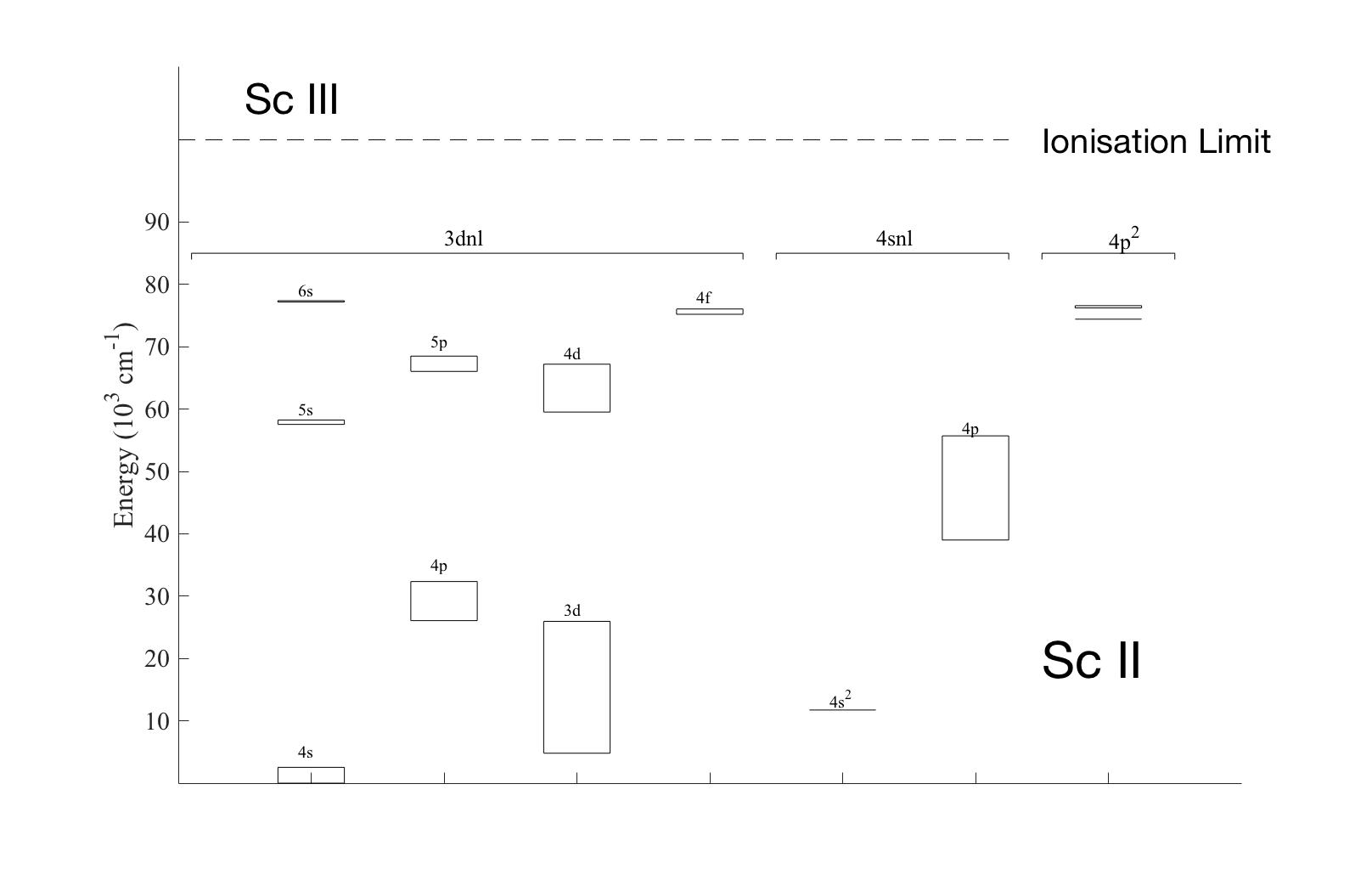
Figure 1: Partial energy level diagram of Sc ii, the energy level values are from Johansson and Litzén (1980). Each box consists of several levels.

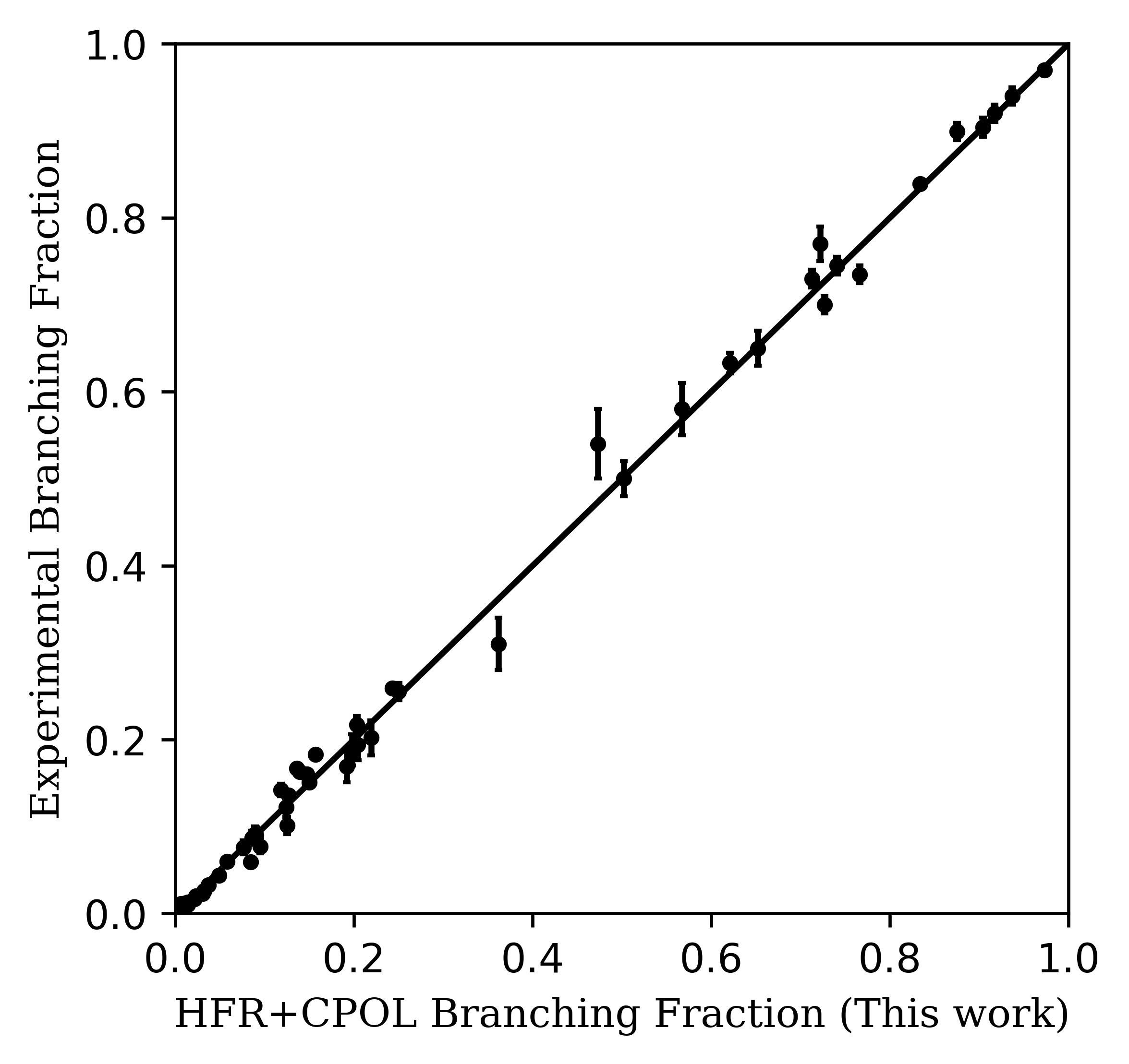
Figure 2: Comparison between the HFR+CPOL branching fractions of this work and the experimental values of Lawler and Dakin (1989). The straight line of equality has been drawn.

The experimental set-up for the two-step Time-Resolved Laser Induced Fluorescence (TR-LIF) measurements at the Lund High Power Laser Facility has been described in detail by Engström et al. (2014) and Lundberg et al. (2016). For an overview we refer to Figure 1 in Lundberg et al. (2016), and here we give only the most important details. A frequency doubled Nd:YAG laser (Continuum Surelite) with 10 ns pulses was used to produce the free scandium ions by focusing the light on a rotating solid scandium sample in a vacuum chamber with a pressure around $10^{-4}$ mbar. The ions in the plasma cone were crossed by two laser beams, a few mm above the solid sample, generating the two-step excitations. The fluorescence signal was detected in a direction perpendicular to both the ablation and excitation lasers.
For the first step (4s-4p), we used a Continuum Nd - 60 dye laser with either DCM or Pyridine 2 dyes. The 10 ns long pulses were frequency doubled using a KDP crystal, giving the wavelengths needed for the first step. The second laser system excited the final high energy levels. It consists of a frequency doubled Continuum NY-82 Nd:YAG laser pumping a Continuum Nd - 60 dye laser with either DCM or Oxacin dye for wavelengths below or above 660 nm, respectively. The pulse length was reduced from 10 ns to less than one ns by stimulated Brillouin scattering. The output was frequency doubled using a KDP crystal and, where higher energy was needed, tripled with a BBO crystal.
For two step excitation, the timing between the pulses is crucial. For this purpose, a delay generator ensures that the second step is timed to when the population of the intermediate state is at its flat maximum as determined by observing the decay of this level in another channel, see Figure 2 in Lundberg et al. (2016).
The fluorescence emitted by the scandium ions was filtered by a 1/8 m grating monochromator with its 0.28 mm wide entrance slit oriented parallel to the excitation laser beams. This fluorescence light was recorded using a fast micro-channel-plate photomultiplier tube (Hamamatsu R3809U) and digitised using a Tektronix DPO 7254 oscilloscope with 2.5 GHz analog bandwidth. We used the second spectral order with a 0.5 nm observed line width for all measurements. The excitation laser pulse shape was recorded simultaneously using a fast photo diode and digitised by another channel of the oscilloscope. All decay curves were averaged over 1000 laser pulses and analysed using the DECFIT software (Palmeri et al., 2008) by fitting a single exponential function convoluted by the measured shape of the second-step laser pulse and a background function to the observed decay.
The excitation schemes of the measured Sc ii levels are presented in Table 1. This table shows the intermediate levels and their excitation wavelengths, the final levels and their excitation wavelengths from the intermediate levels together with the detection channel level and wavelength. For the levels 4d ³S₁, 4d ¹D₂ and 4p^{2 3}P₂, it was possible to record the the decay in more than one channel. We did not find any differences in the lifetimes obtained from the different channels. Sc ii is a complex spectrum with a dense level structure, as shown in Figure 1. Line blending can be caused by cascades or fluorescence from the intermediate level as discussed by Lundberg et al. (2016). For all measurements, we investigated if there was a line blend affecting the recorded curves. Due to the small spectral width of the laser compared to the energy level separations, we avoid exciting multiple levels.
To investigate any possible saturation effects in the second step excitation, a set of neutral density filters was placed in the excitation beam. The delay between the ablation and first excitation pulse, the geometrical alignment of the lasers in respect to the target as well as the intensity of the ablation laser were varied to test time-of-flight effects. No systematic effects were observed.
As discussed in Palmeri et al. (2008), the weighting of individual data points, hence the purely statistical uncertainty in the fitted lifetime, is difficult to estimate accurately because the digitising process is not strictly a counting measurement. However, extensive tests have shown that even for weak lines the dominating factor is the variation between different measurements. The uncertainty in Table 2 represents the uncertainty of 10-20 measurements performed over several days. The difference between subsequent curves is significantly lower than the quoted uncertainty, usually less than 1$\%$.

3 Branching fraction measurements

A water-cooled hollow cathode discharge lamp (HCL) was used to produce the free scandium ions. The lamp has an iron cathode with anodes on each side, separated by glass cylinders. A small piece of scandium was placed in the cathode. We used argon, with a pressure of 0.3 Torr, as a buffer gas and applied currents ranging from 0.2 to 0.5 A. These measurements at different currents are very important to find and compensate for self-absorption effects. If self-absorption is not treated correctly, the measured relative line intensity may be less than the true intensity of the line. This in turn changes the branching fraction which is essential to derive oscillator strengths. Self-absorption was observed in the case of the ${\rm 3d4d~{}^{3}D_{3}}$, ${\rm 3d4d~{}^{3}S_{1}}$, and ${\rm 3d4d~{}^{3}P_{2}}$ levels, and the affected lines were corrected. More details on this procedure can be found in Pehlivan et al. (2015).
The spectra were recorded with the vacuum ultraviolet Fourier transform spectrometer (VUV FTS) at the Blackett Laboratory, Imperial College London (Pickering, J.C., 2002) in the interval $23500-63100$ $\text{cm}^{-1}$ ($425-158$ nm) using a resolution of 0.039 cm^-1. We used two different photomultiplier tube detectors: Hamamatsu R7154 and R11568, the latter with a UG5 filter. Each scandium measurement consists of 12 co-added scans. To determine the relative response functions of the system, we used standard lamps: a tungsten filament lamp ($800-300$ nm) and a deuterium lamp ($410-116$ nm) for the wavelength region ($425-210$ nm), and a deuterium standard lamp alone for the region ($317-158$ nm). The tungsten lamp was calibrated by the UK National Physical Laboratory and the deuterium lamp by Physikalisch-Technische Bundesanstalt, in Berlin. In the region where the lamps overlap, the response functions were placed on the same relative scale. We recorded the spectrum of the calibration lamps immediately before and after each scandium measurement. The HCL and the calibration lamps were placed at the same distances from the FTS, and a mirror was used to select the light source without moving the lamps.
In astrophysics, oscillator strengths ($f$-values) or $\log(gf)$ values are the parameters used for abundance analysis. The $f$-value is proportional to the transition probability for E1 transitions by

$$f=\frac{g_{\text{u}}}{g_{\text{l}}}\lambda^{2}A_{\text{ul}}1.499\times 10^{-16},$$ (1)

where $g_{\text{u}}$ is the statistical weight of the upper level, $g_{\text{l}}$ the statistical weight of the lower level, $\lambda$ the wavelength of the transition in Å, and $A_{\text{ul}}$ the transition probability in s^-1.
The transition probability is related to the branching fraction ($BF$) and the lifetime of the upper level ($\tau_{\text{u}}$). It can be derived using

$$A_{\text{ul}}=\frac{BF_{\text{ul}}}{\tau_{\text{u}}}.$$ (2)

We obtained the lifetimes of the upper levels from our measurements, as discussed in Section 2. The $BF$ is the parameter we measure and it is defined as the transition probability of the line, $A_{\text{ul}}$, divided by the sum of transition probabilities of all lines from the same upper level;

$$BF_{\text{ul}}=\frac{A_{\text{ul}}}{\sum_{i}A_{\text{ui}}}=\frac{I_{\text{ul}}}{\sum_{i}I_{\text{ui}}}.$$ (3)

Since all lines emanate from the same upper level, the transition probability is proportional to the line intensity, $I_{\text{ul}}$, which for FTS spectra is proportional to photon flux (Davis S.P. et al., 2001). Therefore, we derived $BF$s from calibrated intensity ratios in our measurements. All lines were identified using the analysis of Johansson and Litzén (1980). The intensities of the observed lines were determined by fitting Gaussian line profiles using GFit (Engström, 1998, 2014).
The uncertainty of the $A$-value, and thus of the $f$-value, arises from the uncertainty in the upper level lifetime and the uncertainty of the $BF$. The latter includes the uncertainty in the intensity calibration procedure and the uncertainty in the measured line intensity, including the self-absorption correction. The uncertainties of the integrated line intensities were determined using GFit. The relative uncertainties are as low as 0.1% for strong lines and 4% on average. However, for two weak lines the uncertainty is as large as $20\%$. The uncertainty in the calibration using the tungsten lamp is 2.2% and the uncertainty using the deuterium lamp is 8.6% for the region $425-210$ nm and 9.9% between $317$ and $158$ nm. These calibration lamp uncertainties include the calibration uncertainty and the variation resulting from the repeated measurements made before and after all scandium scans. The uncertainties of the radiative lifetimes are given in Table 2. Finally, we were not able to observe the weakest lines from the investigated level. However, we included their contributions as residuals with derived theoretical $BF$s from our calculations. The residual $BF$s are less than $7\%$ for all levels. The uncertainties in the residuals were estimated to $50\%$ and included in the error budget. The final uncertainties in the oscillator strengths are presented in Table 3 and were derived from the individual contributions using the method described by Sikström et al. (2002).

4 Radiative parameter calculations

To calculate branching fractions and the oscillator strengths in Sc ii, we used the relativistic Hartree–Fock (HFR) method implemented in the Cowan’s suite of atomic structure computer codes (Cowan, 1981). It is modified by including a pseudo-potential and a correction to the electric dipole operator that take into account the core-polarisation effects giving rise to the HFR+CPOL technique (Quinet et al., 1999).
In this study, the valence-valence correlation was included using the following configuration interaction (CI) expansions: ${\rm 3d4s}$ + ${\rm 3d5s}$ + ${\rm 3d6s}$ + ${\rm 3d7s}$ + ${\rm 3d^{2}}$ + ${\rm 3d4d}$ + ${\rm 3d5d}$ + ${\rm 3d6d}$ + ${\rm 3d7d}$ + ${\rm 3d5g}$ + ${\rm 3d6g}$ + ${\rm 3d7g}$ + ${\rm 4s^{2}}$+${\rm 4s5s}$ + ${\rm 4s6s}$ + ${\rm 4s7s}$ + ${\rm 4s4d}$ + ${\rm 4s5d}$ + ${\rm 4s6d}$ + ${\rm 4s7d}$ + ${\rm 4s5g}$ + ${\rm 4s6g}$ + ${\rm 4s7g}$ + ${\rm 4p^{2}}$ + ${\rm 4d^{2}}$ + ${\rm 4f^{2}}$ + ${\rm 4p4f}$ for the even parity; ${\rm 3d4p}$ + ${\rm 3d5p}$ + ${\rm 3d6p}$ + ${\rm 3d7p}$ + ${\rm 3d4f}$ + ${\rm 3d5f}$ + ${\rm 3d6f}$ + ${\rm 3d7f}$ + ${\rm 3d6h}$ + ${\rm 3d7h}$ + ${\rm 4s4p}$ + ${\rm 4s5p}$ + ${\rm 4s6p}$ + ${\rm 4s7p}$ + ${\rm 4s4f}$ + ${\rm 4s5f}$ + ${\rm 4s6f}$ + ${\rm 4s7f}$ + ${\rm 4s6h}$ + ${\rm 4s7h}$ + ${\rm 4p4d}$ + ${\rm 4d4f}$ for the odd parity.
Regarding the core-polarisation effects, a Sc iv ${\rm 3p^{6}}$ closed-subshell ionic core was considered where the dipole polarisability, $\alpha_{\text{d}}=2.129$ $a_{0}^{3}$ was taken from the RRPA calculations of Johnson et al. (1983) and a cut-off radius of 1.17 $a_{0}$ was estimated as the HFR mean radius of the outermost 3p orbital, $\left\langle 3p|r|3p\right\rangle_{\text{HFR}}$.
During a least-squares-fit procedure, we adjusted some radial integrals to minimise the discrepancies between the hamiltonian eigenvalues and the experimental energy levels taken from the NIST Atomic Spectra Database (Kramida et al., 2015). The latter are based on the term analysis originally carried out by Russell and Meggers (1927) and later revised by Neufeld (1970) and by Johansson and Litzén (1980). There are 168 levels belonging to the configurations ${\rm 3d4s}$, ${\rm 3d^{2}}$, ${\rm 3d4p}$, ${\rm 4s4p}$, ${\rm 3d5s}$, ${\rm 3d4d}$, ${\rm 3d5p}$, ${\rm 4p^{2}}$, ${\rm 3d4f}$, ${\rm 3d6s}$, ${\rm 4s5s}$, ${\rm 3d5d}$, ${\rm 4s4d}$, ${\rm 3d5f}$, ${\rm 3d5g}$, ${\rm 3d7s}$, ${\rm 3d6d}$, and ${\rm 3d6f}$. The average energies, $E_{\text{av}}$, of the above-mentioned known configurations along with their direct, $F^{k}$, exchange, $G^{k}$, electrostatic and spin-orbit, $\zeta$, radial parameters were considered in the fit of the energy levels. The ab initio and fitted parameter values are reported in Tables 4 and 5 for the even and odd configurations, respectively. The spin-orbit integrals not presented in these tables were fixed to their HFR+CPOL values. The other Slater integrals, including the CI $R^{k}$ parameters, not reported here, were fixed to 80% of their ab initio values to account for missing CI effects (Cowan, 1981). The average deviations of the least-squares-fits were 157 cm^-1 for the 93 even-parity experimental levels and 65 cm^-1 for the 75 odd-parity experimental levels.

5 Results and discussion

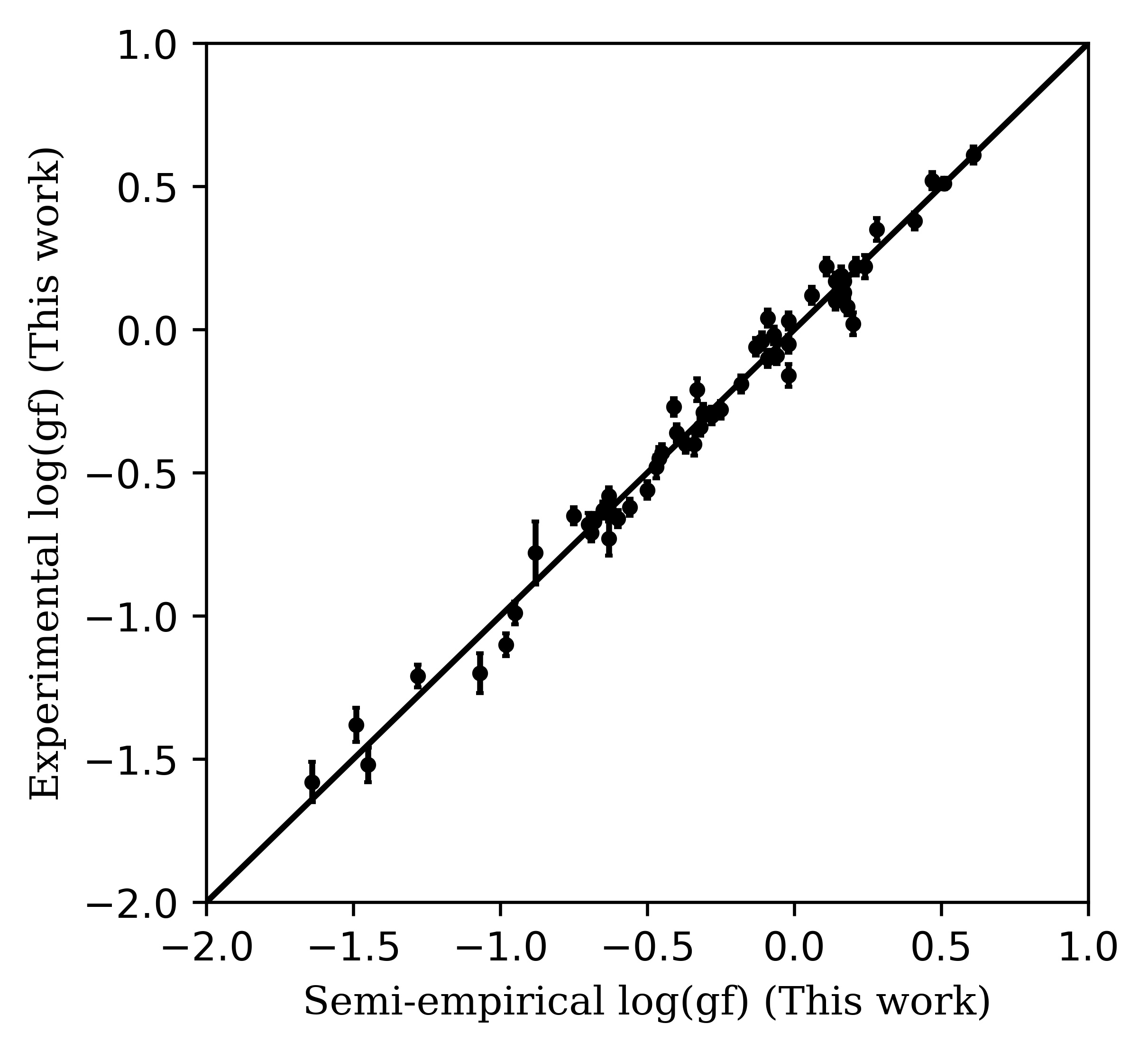
Figure 3: Comparison between the oscillator strengths determined by the combination of the HFR+CPOL branching fractions and the TR-LIF lifetimes of this work and the experimental oscillator strengths derived in this work. The straight line of equality has been drawn.

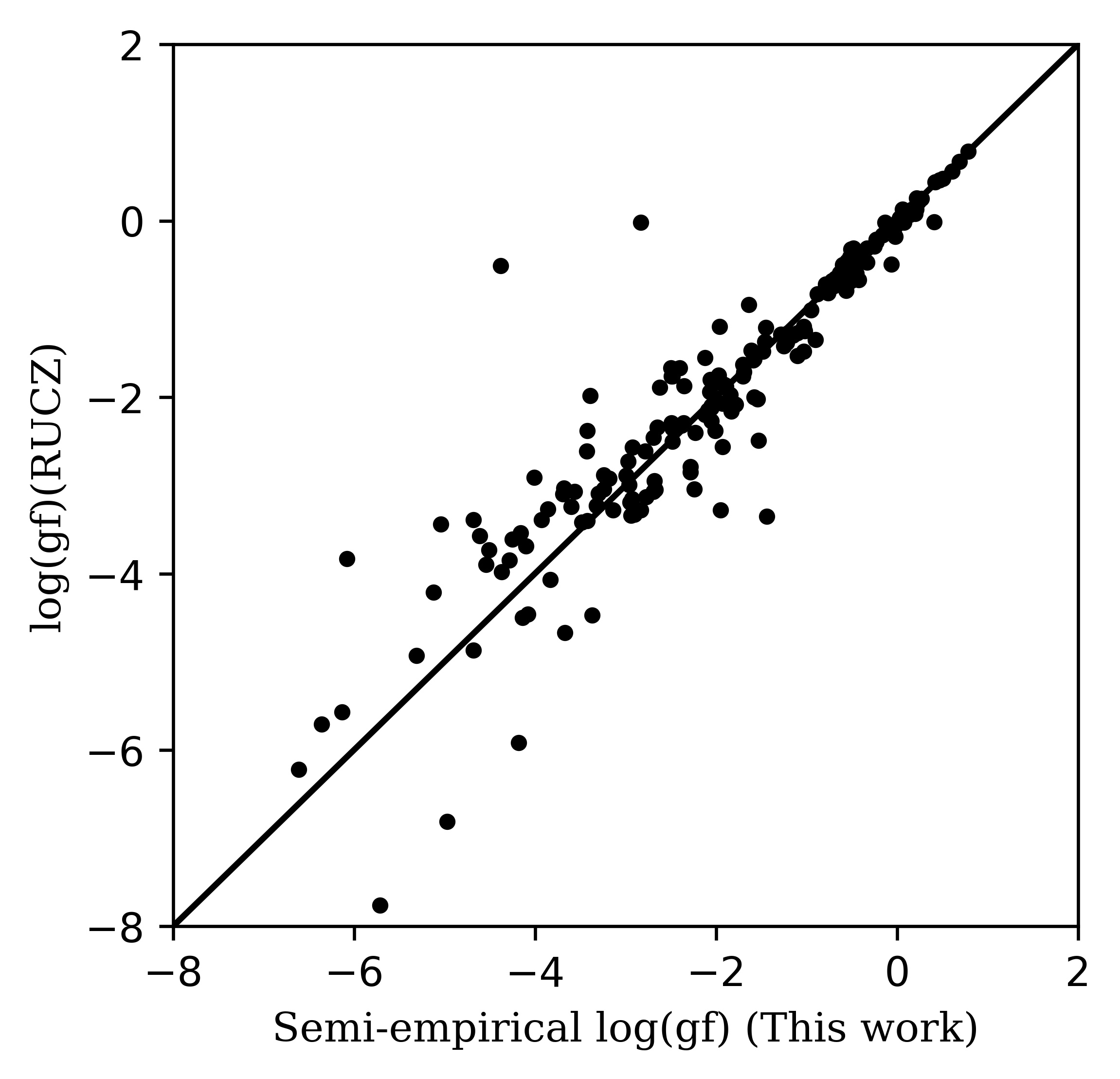
Figure 4: Comparison between the oscillator strengths determined by the combination of the HFR+CPOL branching fractions and the TR-LIF lifetimes (This Work) and the semi-empirical oscillator strengths calculated by Ruczkowski et al. (2014) (RUCZ). The straight line of equality has been drawn.

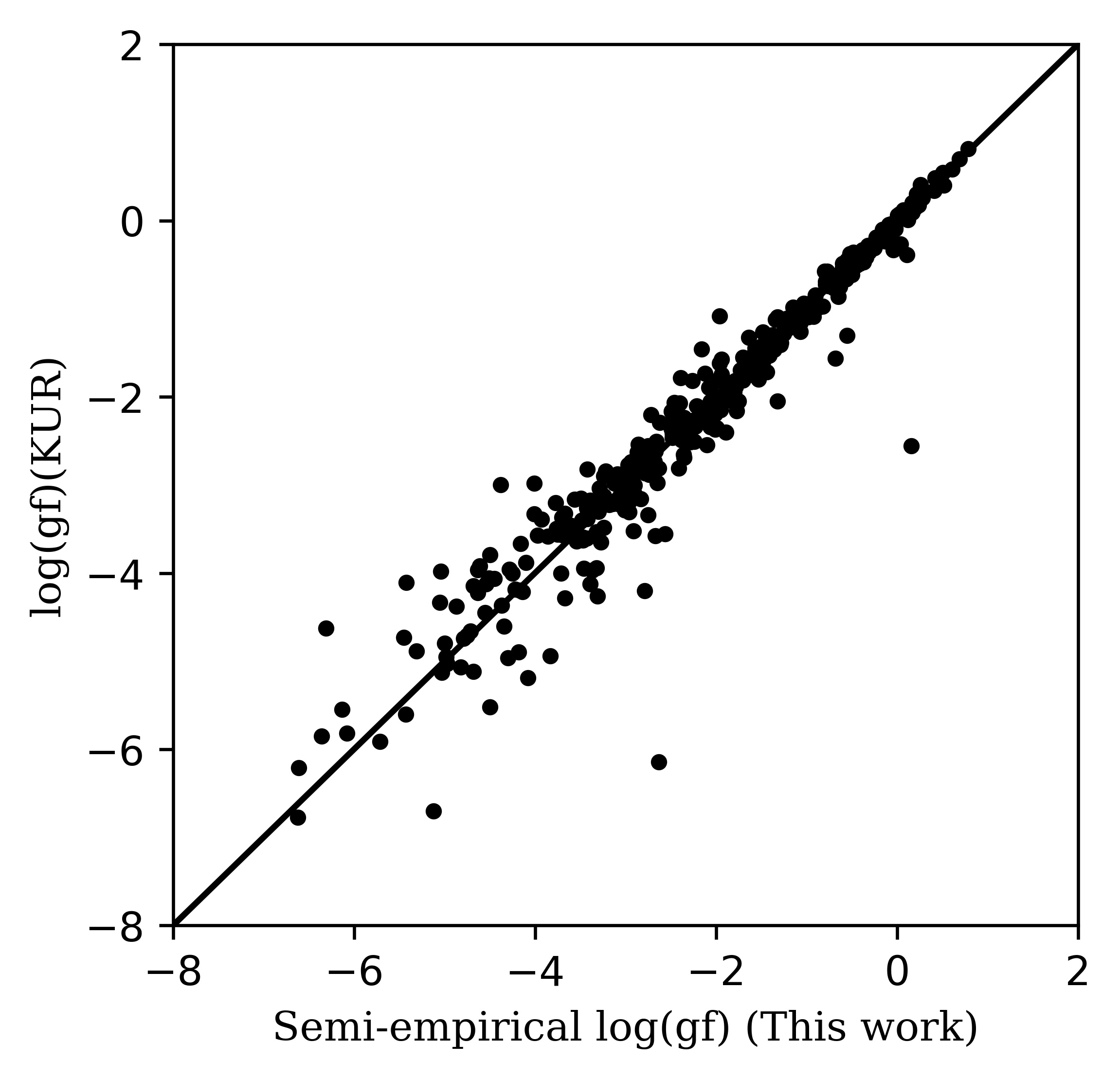
Figure 5: Comparison between the oscillator strengths determined by the combination of the HFR+CPOL branching fractions and the TR-LIF lifetimes (This Work) and the oscillator strengths calculated by Kurucz (2011) (KUR). The straight line of equality has been drawn.

Table 2 compares our TR-LIF and HFR+CPOL lifetimes with other experimental values from the literature (Buchta et al., 1971; Arnesen et al., 1976; Palenius et al., 1976; Vogel et al., 1985; Marsden et al., 1988), the Hartree-Fock values calculated by Kurucz (2011) and the lifetimes deduced from the semi-empirical oscillator strengths calculated by Ruczkowski et al. (2014). On average, our HFR+CPOL lifetimes are shorter than the measurements for the odd-parity levels and longer for the even-parity levels. The discrepancies range from a few percent to about 20%, except for the even-parity levels ${\rm 4p^{2}~{}^{1}D_{2}}$ and ${\rm 3d6s~{}^{3}D_{3}}$ where they reach 57% and 49%, respectively. In the former case, this state is strongly mixed (our calculation gives 36% ${\rm 4p^{2}~{}^{1}D_{2}}$ + 36% ${\rm 4s4d~{}^{1}D_{2}}$ + 23% ${\rm 3d6s~{}^{1}D_{2}}$) and an important decay channel (${\rm 4p^{2}~{}^{1}D_{2}\rightarrow 3d4p~{}^{1}D^{o}_{2}}~{}~{}BF=0.0713$) is affected by cancellation (the cancellation factor as defined by Cowan (1981) is less than 5%) that could explain the over estimated lifetime. Concerning ${\rm 3d6s~{}^{3}D_{3}}$ level, no such argument could explain the observed disagreement. The beam-foil measurements of Buchta et al. (1971) can be rejected for the levels ${\rm 3d4p~{}^{3}D^{o}_{3},^{1}P^{o}_{1},^{1}F^{o}_{3}}$ as previously stated by Marsden et al. (1988) due to blending problems.
The calculations by Kurucz (2011) show roughly the same systematic discrepancy with experiment (lifetimes shorter for the odd parity and longer for the even parity) as our HFR+CPOL calculations. Although the calculation of Kurucz (2011) shows a better agreement than HFR+CPOL for certain 3d4d levels (${\rm{}^{3}F_{2,4}}$, ${\rm{}^{1}D_{2}}$, ${\rm{}^{3}P_{2}}$), it does not solve the theory-experiment disagreements observed for the levels ${\rm 4p^{2}~{}^{1}D_{2}}$ and ${\rm 3d6s~{}^{3}D_{3}}$. The parametric calculation of Ruczkowski et al. (2014) agrees with our HFR+CPOL model within 10% including all levels. Unfortunately, no lifetime value can be deduced from Ruczkowski et al. (2014) for the levels ${\rm 4p^{2}~{}^{1}D_{2}}$ and ${\rm 3d6s~{}^{3}D_{3}}$. Concerning the level ${\rm 3d4d~{}^{3}G_{3}}$, our TR-LIF measurement is slightly lower than the one of Marsden et al. (1988) although the error bars do overlap.
For all 3d4p levels, our HFR+CPOL model and the parametric calculation of Ruczkowski et al. (2014) are closer to the measurement of Marsden et al. (1988). The excellent agreement between Marsden et al. (1988) and Ruczkowski et al. (2014) is not surprising as the latter adjusted the dipole transition integrals to the oscillator strengths determined from the branching fraction measurements of Lawler and Dakin (1989) combined with the lifetime measurements of Marsden et al. (1988). For most of the higher levels, the lifetimes calculated by Kurucz (2011) are closer to our measurements than those of Ruczkowski et al. (2014).
Although there is a systematic discrepancy between the theoretical and experimental lifetimes, we find a better agreement when comparing our calculated $BF$s with the experimental values. For the high excitation lines, measured in this work, the averaged $BF$ ratio is $1.02\pm 0.16$ with respect to the calculated values. Similarly, Figure 2 shows the good agreement between $BF$s computed in this study using the HFR+CPOL method and the measurements by Lawler and Dakin (1989). Here, the averaged $BF$ ratio is $0.98\pm 0.20$. Based on these comparisons, the calculated $BF$s were combined with our TR-LIF lifetimes and those of Marsden et al. (1988) to determine rescaled transition probabilities and oscillator strengths.
In Table 3, we present our experimental $\log(gf)$ values, together with the measured $BF$s, the uncertainties and the corresponding rescaled theoretical oscillator strengths, $\log(gf)_{\text{resc}}$. Figure 3 illustrates the final agreement between our experimental $\log(gf)$ values and the calculated $\log(gf)_{\text{resc}}$. Table 6 summarises our calculated radiative parameters along with the weighted transition probabilities ($gA$), the weighted oscillator strengths in the log scale ($\log(gf)$), the HFR+CPOL branching fractions ($BF$), and the cancellation factor ($CF$) as defined by Cowan (1981).
Our rescaled theoretical oscillator strengths are compared to the semi-empirical values calculated by Ruczkowski et al. (2014) in Figure 4. As expected, the scatter increases for the weak lines, i.e. the transitions with $\log(gf)\lesssim-1$, where cancellation effects could be an issue. For instance, the transition ${\rm 3d4p~{}^{3}P^{o}_{2}-4p^{2}~{}^{3}P_{2}}$ labelled in Table 6 $76589(e)2-29824(o)2$ has a very low cancellation factor ($CF=0.001$) that indicates a strong cancellation effect in our HFR+CPOL line strength calculation. Indeed, the rescaled oscillator strength for that transition is $\log(gf)_{\text{resc}}=-2.83$ which is three orders of magnitude lower (in the linear scale) than the value predicted by Ruczkowski et al. (2014) ($\log(gf)=-0.02$). On the other hand, a transition for which the cancellation effects in our model is not an issue ($CF>0.05$) such as ${\rm 3d4p~{}^{3}F^{o}_{3}-3d4d~{}^{3}F_{4}}$ ($63529(e)4-27602(o)3$) has an oscillator strength predicted by Ruczkowski et al. (2014) ($\log(gf)=-3.35$) that is two orders of magnitude lower than our rescaled value ($\log(gf)_{\text{resc}}=-1.44$). This could indicate a strong cancellation effect in their calculation. Unfortunately, they did not estimate any cancellation factors. For the strongest transitions, i.e. ${\log(gf)}\gtrsim-1$, the mean scatter drops to about 20% in the linear scale.
In Figure 5, our semi-empirical values are compared to the calculation of Kurucz (2011) where a similar global correlation is observed. The mean scatter in this case is also found to be $\sim$20% for transitions with $\log(gf)\gtrsim-1$ and increases for weaker lines. Here again, the cancellation factors are not available in Kurucz’s database (Kurucz, 2011). But, for example, our predicted strong line ${\rm 3d5p~{}^{3}F^{o}_{3}-3d6s~{}^{3}D_{3}}$ ($77387(e)3-66564(o)3$) with $\log(gf)_{\text{resc}}=0.16$ and $CF=0.379$ is certainly affected by a strong cancellation effect in the calculation of Kurucz (2011) dramatically lowering its oscillator strength to $\log(gf)=-2.56$.
Based on the differences between different sets of $BF$s discussed above and including the uncertainties of the experimental lifetimes, we estimate the accuracy of the rescaled theoretical $f$-values to be $10\%$ for the strong lines and $15-20\%$ for other lines.

6 Consequence on the Solar abundance of scandium

Scott et al. (2015) have redetermined the solar abundances of the iron-peak elements employing a 3D model atmosphere that takes into account departures from the local thermodynamic equilibrium. However, the significant discrepancy between the photospheric and the meteoritic abundances (Lodders et al., 2009) still remains for scandium with ${\rm log}~{}\epsilon_{\sun}=3.16\pm 0.04$ and ${\rm log}~{}\epsilon_{\text{met}}=3.05\pm 0.02$.
The Sc ii lines used in Scott et al. (2015) for the determination of the solar abundance of scandium are presented in Table 7. These lines are from low-excited levels measured by Lawler and Dakin (1989) but not included in our present study. The third column of this table contains the oscillator strengths deduced from the $A$-values of Lawler and Dakin (1989) used by Scott et al. (2015) to determine the photospheric abundances listed in sixth column. They are compared to our rescaled oscillator strengths reported in the fourth column and the differences between the two values are given in the log scale in the fifth column. For this set of solar lines, our oscillator strengths are systematically larger than those of Lawler and Dakin (1989) by $\sim$0.1 dex on average, if we exclude the transition ${\rm 3d^{2}~{}^{1}D_{2}-3d4p~{}^{1}D^{o}_{2}}$ for which our $f$-value is affected by strong cancellation effects. Column seven in Table 7 gives the abundances obtained from each line, assuming they are all lying on the linear part of the curve of growth (see the upper left panel of Figure 3 in Scott et al. (2015)), with our new $gf$-values.
The weighted average along with the corresponding weighted standard deviation of the abundance were determined using the weights of Scott et al. (2015), reported in the last column of Table 7. Their weights range from one to three and are based on the line quality for abundance determination. Discarding the line ${\rm 3d^{2}~{}^{1}D_{2}-3d4p~{}^{1}D^{o}_{2}}$ from the mean estimate, one obtains ${\rm log}~{}\epsilon_{\text{cor}}=3.04\pm 0.13$ (where the second number is the standard deviation) for the corrected photospheric abundance, now in good agreement with the meteoritic value of Lodders et al. (2009). Even if we reject the transition ${\rm 3d^{2}~{}^{3}F_{4}-3d4p~{}^{3}F^{o}_{3}}$ for which there is a factor of two difference between our rescaled $f$-value and the experimental value of Lawler and Dakin (1989), the mean ${\rm log}~{}\epsilon_{\text{cor}}=3.10\pm 0.05$ is still in accord with the meteoritic value. Moreover, considering the full line set does not change the agreement (${\rm log}~{}\epsilon_{\text{cor}}=3.07\pm 0.17$). Finally we note that, all these weighted average abundances agree within the mutual error bars with the value determined by Scott et al. (2015) using only Sc i lines (${\rm log}~{}\epsilon=3.14\pm 0.09$).
Replacing our $f$-value set by the one of Kurucz (2011) will not change this accord either (${\rm log}~{}\epsilon_{\text{kur}}=3.10\pm 0.09$). This is not the case for the set of Ruczkowski et al. (2014). Indeed, the photospheric abundance would be estimated significantly too high with respect to the meteoritic value, i.e. ${\rm log}~{}\epsilon_{\text{ruc}}=3.44\pm 0.31$. Even if the transition ${\rm 3d^{2}~{}^{3}F_{4}-3d4p~{}^{3}F^{o}_{3}}$ for which the oscillator strength calculated by Ruczkowski et al. (2014) ($\log(gf)_{\text{ruc}}=-3.28$) is one order of magnitude lower than the experimental value of Lawler and Dakin (1989) is excluded, this would not significantly improve the situation (${\rm log}~{}\epsilon_{\text{ruc}}=3.29\pm 0.01$).
It should be noted, however, that the lines used for these studies are weak, see Figure 6. Their $BFs$ are less than $5\%$ except for $\lambda 566.904$ having $\sim 10\%$. These small $BFs$ make it difficult to measure and calculate with high accuracy. The real uncertainty might thus be larger than the observed scatter.

7 Conclusions

New TR-LIF lifetimes were measured using two-step excitation schemes in Sc ii. These measurements extend the set of available experimental values with 17 even-parity levels belonging to the excited configurations ${\rm 3d5s}$, ${\rm 3d4d}$, ${\rm 4p^{2}}$ and ${\rm 3d6s}$. We measured 57 $BFs$ from these upper levels using a HCL and a FTS. By combining the $BFs$ with the measured lifetimes, we derived $\log(gf)$ values from these highly-excited levels. A Hartree-Fock model that includes the main relativistic interactions along with the core-polarisation effects (HFR+CPOL) was used to determine the branching fractions and the oscillator strengths. The comparison between our HFR+CPOL and TR-LIF lifetimes along with those found in the literature (Buchta et al., 1971; Arnesen et al., 1976; Palenius et al., 1976; Vogel et al., 1985; Marsden et al., 1988; Ruczkowski et al., 2014; Kurucz, 2011) shows generally a good agreement ranging from a few percent to 20% with the notable exceptions of the even-parity levels ${\rm 4p^{2}~{}^{1}D_{2}}$ and ${\rm 3d6s~{}^{3}D_{3}}$. The former discrepancy may be due to a cancellation effect that lengthens the HFR+CPOL lifetime. Owing to the good agreement ($\sim$20%) obtained with the experimental branching fractions of Lawler and Dakin (1989) for low-excitation levels and ours for high-excitation levels, the HFR+CPOL branching fractions were combined with our TR-LIF lifetimes and the experimental values of Marsden et al. (1988) to obtain rescaled semi-empirical oscillator strengths for all the 380 E1 transitions depopulating the 34 fine-structure levels for which TR-LIF lifetimes are available. This new set of oscillator strengths were compared to the parametric calculation of Ruczkowski et al. (2014) and to the Hartree-Fock values of Kurucz (2011). In both cases, the mean scatters were $\sim$20% for the strong lines ($\log(gf)\gtrsim-1$) giving an estimate of the accuracy for these radiative parameters. Finally, the solar abundance of scandium was estimated to ${\rm log}~{}\epsilon_{\sun}=3.04\pm 0.13$ using our rescaled semi-empirical oscillator strengths to correct the values determined in the recent study of Scott et al. (2015). This value is in improved agreement with the meteoritic value (${\rm log}~{}\epsilon_{\text{met}}=3.05\pm 0.02$) of Lodders et al. (2009).

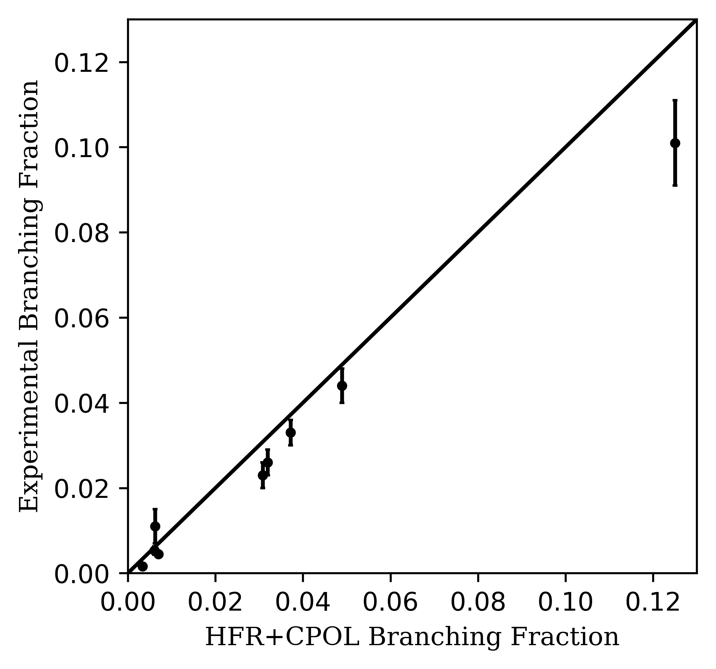
Figure 6: Comparison between the HFR+CPOL branching fractions and the experimental values of Lawler and Dakin (1989) for the Sc ii lines used in the determination of the solar scandium abundance. The straight line of equality has been drawn.

Table 1: Measured Sc ii levels and the corresponding two$-$step excitation schemes

Final	First Step Excitation			Second Step Excitation			Detection
Levela	Starting	Intermediate	$\lambda_{air}$	Final Levela	$\lambda_{air}$	Schemeb	Lower Levela	$\lambda_{air}$
	Levela (cm-1)	Levela (cm-1)	(nm)	(cm-1)	(nm)		(cm-1)	(nm)
5s 3D3	67.72	27602.45	363.07	57743.92	331.67	2$\omega$	27841.35	334.32
5s 1D2	67.72	27602.45	363.07	58252.09	326.17	2$\omega$	32349.98	385.96
4d 1F3	177.76	29823.93	337.22	59528.42	336.55	2$\omega$	26081.34	298.89
4d 3D1	177.76	29823.93	337.22	59875.08	332.67	2$\omega$	27917.78	312.83
4d 3D2	177.76	29823.93	337.22	59929.46	332.07	2$\omega$	28021.29	313.31
4d 3D3	177.76	29823.93	337.22	60001.91	331.27	2$\omega$	28161.17	313.97
4d 3G3	177.76	29823.93	337.22	60267.16	328.39	2$\omega$	27443.71	304.57
4d 1P1	177.76	29823.93	337.22	60400.41	326.95	2$\omega$	26081.34	291.30
4d 3S1	177.76	29823.93	337.22	61071.43	319.93	2$\omega$	29823.93	319.93
							39345.52	460.15
4d 3F2	2540.95	32349.98	335.37	63374.63	322.23	2$\omega$	27917.78	281.95
4d 3F4	2540.95	32349.98	335.37	63528.54	320.64	2$\omega$	28161.17	282.66
4d 1D2	2540.95	32349.98	335.37	64366.68	312.25	2$\omega$	26081.34	261.12
							30815.70	297.97
4d 3P2	2540.95	32349.98	335.37	64705.89	308.98	2$\omega$	29823.93	286.60
4p2 1D2	177.76	28161.17	357.25	74433.30	216.04	3$\omega$	32349.98	237.55
4p2 3P1	177.76	29823.93	337.22	76360.80	214.82	3$\omega$	39345.52	270.08
4p2 3P2	177.76	29823.93	337.22	76589.30	213.76	3$\omega$	28161.17	206.43
							39115.04	266.77
							39345.52	268.42
6s 3D3	177.76	29823.93	337.22	77387.17	210.18	3$\omega$	28161.17	203.08

^a All energy level values and wavelength values are from Johansson and Litzén (1980).
^b $2\omega$ and $3\omega$ stand for, respectively, frequency doubling and tripling excitation schemes. All first step levels are excited using a frequency doubling scheme (2$\omega$)

Table 2: Comparison of radiative lifetimes ($\tau$) in Sc ii

Levela	$E^{a}$	$\tau_{\text{this~{}cal}}^{b}$	$\tau_{\text{this~{}exp}}^{c}$	$\tau_{\text{other~{}exp}}$	$\tau_{\text{other~{}cal}}$
	(cm-1)	(ns)	(ns)	(ns)	(ns)
${\rm 3d4p~{}^{1}D^{o}_{2}}$	26081.34	6.65		7.5$\pm$0.4d	6.54i
				7.16$\pm$0.18e	7.79j
				7.8$\pm$0.8h
${\rm 3d4p~{}^{3}F^{o}_{2}}$	27443.71	5.68		6.2$\pm$0.3d	5.38i
				6.2$\pm$0.2f	5.90j
				6.5$\pm$0.4g
${\rm 3d4p~{}^{3}F^{o}_{3}}$	27602.45	5.62		6.1$\pm$0.3d	5.32i
					5.83j
${\rm 3d4p~{}^{3}F^{o}_{4}}$	27841.35	5.54		6.1$\pm$0.3d	5.24i
				5.6$\pm$0.6h	5.75j
${\rm 3d4p~{}^{3}D^{o}_{1}}$	27917.78	4.44		4.7$\pm$0.2d	4.20i
				4.61$\pm$0.10e	4.67j
${\rm 3d4p~{}^{3}D^{o}_{2}}$	28021.29	4.41		4.7$\pm$0.2d	4.17i
				4.66$\pm$0.14e	4.64j
${\rm 3d4p~{}^{3}D^{o}_{3}}$	28161.17	4.38		4.7$\pm$0.2d	4.15i
				4.55$\pm$0.15e	4.59j
				6.1$\pm$0.6h
${\rm 3d4p~{}^{3}P^{o}_{0}}$	29736.27	6.36		7.7$\pm$0.4d	6.80i
				7.48$\pm$0.18e	7.44j
${\rm 3d4p~{}^{3}P^{o}_{1}}$	29742.16	6.39		7.6$\pm$0.4d	6.76i
				7.3$\pm$0.3e	7.45j
${\rm 3d4p~{}^{3}P^{o}_{2}}$	29823.93	6.30		7.4$\pm$0.4d	6.67i
				7.30$\pm$0.16e	7.50j
${\rm 3d4p~{}^{1}P^{o}_{1}}$	30815.70	8.10		8.8$\pm$0.4d	7.35i
				8.5$\pm$0.6g	8.76j
				5.5$\pm$0.5h
${\rm 3d4p~{}^{1}F^{o}_{3}}$	32349.98	4.68		5.1$\pm$0.3d	4.46i
				5.2$\pm$0.2e	5.20j
				6.8$\pm$0.6h
${\rm 4s4p~{}^{3}P^{o}_{0}}$	39002.20	3.69		3.7$\pm$0.2d	3.36i
					3.66j
${\rm 4s4p~{}^{3}P^{o}_{1}}$	39115.04	3.69		3.7$\pm$0.2d	3.37i
					3.67j
${\rm 4s4p~{}^{3}P^{o}_{2}}$	39345.52	3.70		3.8$\pm$0.2d	3.39i
					3.67j
${\rm 4s4p~{}^{1}P^{o}_{1}}$	55715.36	0.88			0.91i
${\rm 3d5s~{}^{3}D_{1}}$	57551.88	3.49			3.44i
${\rm 3d5s~{}^{3}D_{2}}$	57614.40	3.50			3.44i
${\rm 3d5s~{}^{3}D_{3}}$	57743.92	3.50	3.20$\pm$0.20		3.44i
${\rm 3d5s~{}^{1}D_{2}}$	58252.09	3.70	3.26$\pm$0.20		3.66j
${\rm 3d4d~{}^{1}F_{3}}$	59528.42	2.69	2.32$\pm$0.15		2.51i
					2.51j

Table 2: Continued.

Levela	$E^{a}$	$\tau_{\text{this~{}cal}}^{b}$	$\tau_{\text{this~{}exp}}^{c}$	$\tau_{\text{other~{}exp}}$	$\tau_{\text{other~{}cal}}$
	(cm-1)	(ns)	(ns)	(ns)	(ns)
${\rm 3d4d~{}^{3}D_{1}}$	59875.08	2.72	2.23$\pm$0.15		2.62i
${\rm 3d4d~{}^{3}D_{2}}$	59929.46	2.74	2.32$\pm$0.15		2.63i
					2.58j
${\rm 3d4d~{}^{3}D_{3}}$	60001.91	2.76	2.41$\pm$0.20		2.65i
${\rm 3d4d~{}^{3}G_{3}}$	60267.16	2.50	2.19$\pm$0.15	2.5$\pm$0.2d	2.33i
					2.47j
${\rm 3d4d~{}^{3}G_{4}}$	60348.46	2.52		2.4$\pm$0.2d	2.35i
					2.49j
${\rm 3d4d~{}^{1}P_{1}}$	60400.41	2.89	2.44$\pm$0.15		2.69i
					2.63j
${\rm 3d4d~{}^{3}G_{5}}$	60457.12	2.54		2.5$\pm$0.2d	2.38i
					2.51j
${\rm 3d4d~{}^{3}S_{1}}$	61071.43	2.82	2.45$\pm$0.15		2.77i
					2.78j
${\rm 3d4d~{}^{3}F_{2}}$	63374.63	2.40	2.15$\pm$0.10		2.05i
					2.43j
${\rm 3d4d~{}^{3}F_{3}}$	63445.16	2.41			2.05i
${\rm 3d4d~{}^{3}F_{4}}$	63528.54	2.43	2.19$\pm$0.10		2.07i
					2.47j
${\rm 3d4d~{}^{1}D_{2}}$	64366.68	2.73	2.25$\pm$0.15		2.26i
${\rm 3d4d~{}^{3}P_{0}}$	64615.77	3.21			2.65i
${\rm 3d4d~{}^{3}P_{1}}$	64646.70	3.21			2.65i
${\rm 3d4d~{}^{3}P_{2}}$	64705.89	3.19	2.51$\pm$0.15		2.65i
${\rm 3d4d~{}^{1}G_{4}}$	65236.04	3.17			2.45i
${\rm 3d4d~{}^{1}S_{0}}$	67216.56	3.87			2.74i
${\rm 4p^{2}~{}^{1}D_{2}}$	74433.30	5.96	3.80$\pm$0.15		6.80i
${\rm 4p^{2}~{}^{3}P_{0}}$	76243.20	1.17			1.28i
${\rm 4p^{2}~{}^{3}P_{1}}$	76360.80	1.17	1.14$\pm$0.06		1.28i
${\rm 4p^{2}~{}^{3}P_{2}}$	76589.30	1.18	1.09$\pm$0.06		1.30i
					1.03j
${\rm 3d6s~{}^{3}D_{1}}$	77195.19	5.56			5.00i
${\rm 3d6s~{}^{3}D_{2}}$	77256.99	5.55			5.00i
${\rm 3d6s~{}^{3}D_{3}}$	77387.17	5.54	3.73$\pm$0.25		4.98i
${\rm 3d6s~{}^{1}D_{2}}$	77833.88	6.61			6.94i

^a Johansson and Litzén (1980).
^b HFR+CPOL calculation. This work.
^c TR-LIF measurements. This work.
^d TR-LIF measurements by Marsden et al. (1988).
^e TR-LIF measurements by Vogel et al. (1985).
^f TR-LIF measurements by Arnesen et al. (1976).
^g Beam-foil spectroscopy by Palenius et al. (1976).
^h Beam-foil spectroscopy by Buchta et al. (1971).
ⁱ Hartree-Fock calculation by Kurucz (2011).
^j Parametric method calculation by Ruczkowski et al. (2014).

Table 3: Presentation of experimental $\log(gf)$ values together with the transition, wavelength, $\lambda$, wavenumber, $\sigma$, measured branching fraction, $BF_{\text{exp}}$, experimental transition probability, $A_{\text{exp}}$ , and the corresponding rescaled semi-empirical $\log(gf)$ values of this work. The radiative lifetimes, $\tau$, are TR-LIF measurements from this work.

Upper levela		Lower levela		$\lambda_{\text{exp}}^{a}$	$\sigma_{\text{exp}}^{a}$	$\sigma_{\text{theo}}^{b}$	$BF_{\text{exp}}$	$BF$ unc.	$A_{\text{exp}}$	$\log(gf)$	$\log(gf)_{\text{resc}}$
Config.	Energy (cm-1)	Config.	Energy (cm-1)	(nm)	(cm-1)	(cm-1)		$\%$	(s-1)	Exp.	Calc.
3d5s 3D3	57744	3d4p 3F${}_{3}^{o}$	27602	331.673	30141.50	30176	6.21E-02	4	1.94E+07	-0.65$\pm$0.03	-0.75
$\tau$= 3.20$\pm$0.20 ns		3d4p 3F${}_{4}^{o}$	27841	334.323	29902.57	29944	4.05E-01	3	1.27E+08	0.17$\pm$0.03	0.14
		3d4p 3D${}_{2}^{o}$	28021	336.347	29722.58	29771	5.29E-02	4	1.65E+07	-0.71$\pm$0.03	-0.69
		3d4p 3D${}_{3}^{o}$	28161	337.938	29582.76	29620	3.60E-01	3	1.12E+08	0.13$\pm$0.03	0.17
		3d4p 3P${}_{2}^{o}$	29824	358.064	27919.88	27888	1.20E-01	4	3.75E+07	-0.30$\pm$0.03	-0.28
		Residual					3.37E-03
3d5s 1D2	58252	3d4p 1D${}_{2}^{o}$	26081	310.751	32179.68	32040	4.90E-01	2	1.50E+08	0.04$\pm$0.03	-0.09
$\tau$= 3.26$\pm$0.20 ns		3d4p 3F${}_{2}^{o}$	27444	324.493	30808.34	30866	1.08E-02	16	3.30E+06	-1.58$\pm$0.07	-1.64
		3d4p 1P${}_{1}^{o}$	30816	364.376	27436.43	27508	1.48E-01	4	4.55E+07	-0.34$\pm$0.03	-0.32
		3d4p 1F${}_{3}^{o}$	32350	385.960	25902.13	25865	3.51E-01	5	1.08E+08	0.08$\pm$0.03	0.18
		Residual					2.10E-02
3d4d 1F3	59528	3d4p 1D${}_{2}^{o}$	26081	298.893	33447.17	33296	8.22E-01	0.5	3.54E+08	0.52$\pm$0.03	0.47
$\tau$= 2.32$\pm$0.15 ns		3d4p 3D${}_{3}^{o}$	28161	318.712	31367.21	31408	6.54E-03	14	2.82E+06	-1.52$\pm$0.06	-1.45
		3d4p 1F${}_{3}^{o}$	32350	367.834	27178.50	27121	1.72E-01	7	7.40E+07	0.02$\pm$0.04	0.20
		Residual					5.10E-03
3d4d 3D1	59875	3d4p 3F${}_{2}^{o}$	27444	308.254	32431.14	32475	1.22E-01	5	5.49E+07	-0.63$\pm$0.04	-0.63
$\tau$= 2.23$\pm$0.15 ns		3d4p 3D${}_{1}^{o}$	27918	312.827	31957.28	32026	4.57E-01	3	2.05E+08	-0.04$\pm$0.03	-0.11
		3d4p 3D${}_{2}^{o}$	28021	313.843	31853.76	31913	1.17E-01	5	5.24E+07	-0.63$\pm$0.04	-0.65
		3d4p 3P${}_{0}^{o}$	29736	331.703	30138.84	30134	1.79E-01	4	8.02E+07	-0.40$\pm$0.03	-0.37
		3d4p 3P${}_{1}^{o}$	29742	331.768	30132.91	30123	1.25E-01	5	5.61E+07	-0.56$\pm$0.04	-0.50
		Residual					3.75E-02
3d4d 3D2	59929	3d4p 3F${}_{3}^{o}$	27602	309.249	32327.05	32372	1.21E-01	5	5.23E+07	-0.43$\pm$0.03	-0.45
$\tau$= 2.32$\pm$0.15 ns		3d4p 3D${}_{1}^{o}$	27918	312.296	32011.74	32081	8.39E-02	5	3.62E+07	-0.58$\pm$0.03	-0.63
		3d4p 3D${}_{2}^{o}$	28021	313.309	31908.30	31968	4.12E-01	3	1.78E+08	0.12$\pm$0.03	0.06
		3d4p 3D${}_{3}^{o}$	28161	314.688	31768.28	31816	6.61E-02	5	2.85E+07	-0.67$\pm$0.03	-0.68
		3d4p 3P${}_{1}^{o}$	29742	331.170	30187.30	30178	2.50E-01	4	1.08E+08	-0.05$\pm$0.03	-0.02
		3d4p 3P${}_{2}^{o}$	29824	332.069	30105.53	30084	6.67E-02	5	2.87E+07	-0.62$\pm$0.03	-0.56
		Residual					3.42E-02
3d4d 3D3	60002	3d4p 3F${}_{4}^{o}$	27841	310.850	32160.62	32214	9.39E-02	6	3.90E+07	-0.40$\pm$0.04	-0.34
$\tau$= 2.41$\pm$0.20 ns		3d4p 3D${}_{2}^{o}$	28021	312.599	31980.37	32041	4.35E-02	7	1.81E+07	-0.73$\pm$0.06	-0.63
		3d4p 3D${}_{3}^{o}$	28161	313.972	31840.77	31890	5.16E-01	4	2.14E+08	0.35$\pm$0.04	0.28
		3d4p 3P${}_{2}^{o}$	29824	331.272	30178.03	30157	3.47E-01	5	1.44E+08	0.22$\pm$0.04	0.24
		Residual					3.51E-02

Table 3: Continued.

Upper levela		Lower levela		$\lambda_{\text{exp}}^{a}$	$\sigma_{\text{exp}}^{a}$	$\sigma_{\text{theo}}^{b}$	$BF_{\text{exp}}$	$BF$ unc.	$A_{\text{exp}}$	$\log(gf)$	$\log(gf)_{\text{resc}}$
Config.	Energy (cm-1)	Config.	Energy (cm-1)	(nm)	(cm-1)	(cm-1)		$\%$	(s-1)	Exp.	Calc.
3d4d 3G3	60267	3d4p 3F${}_{2}^{o}$	27444	304.572	32823.36	32822	9.26E-01	1	4.23E+08	0.61$\pm$0.03	0.61
$\tau$= 2.19$\pm$0.15 ns		3d4p 3F${}_{3}^{o}$	27602	306.052	32664.51	32664	7.41E-02	8	3.38E+07	-0.48$\pm$0.04	-0.47
		Residual					6.20E-03
3d4d 1P1	60400	3d4p 1D${}_{2}^{o}$	26081	291.298	34319.09	34206	3.98E-01	7	1.63E+08	-0.21$\pm$0.04	-0.33
$\tau$= 2.44$\pm$0.15 ns		3d4p 1P${}_{1}^{o}$	30816	337.915	29584.65	29673	6.02E-01	5	2.47E+08	0.10$\pm$0.03	0.14
		Residual					7.27E-02
3d4d 3S1	61071	3d4p 3P${}_{0}^{o}$	29736	319.038	31335.12	31336	1.13E-01	7	4.60E+07	-0.68$\pm$0.04	-0.70
$\tau$= 2.45$\pm$0.15 ns		3d4p 3P${}_{1}^{o}$	29742	319.098	31329.24	31326	2.84E-01	6	1.16E+08	-0.28$\pm$0.04	-0.25
		3d4p 3P${}_{2}^{o}$	29824	319.933	31247.50	31231	5.73E-01	4	2.34E+08	0.03$\pm$0.03	-0.02
		3d4p 1P${}_{1}^{o}$	30816	330.421	30255.76	30319	3.04E-02	10	1.24E+07	-1.21$\pm$0.05	-1.28
		Residual					6.10E-02
3d4d 3F2	63375	3d4p 3F${}_{2}^{o}$	27444	278.230	35930.81	35960	3.57E-01	5	1.66E+08	-0.02$\pm$0.03	-0.07
$\tau$= 2.15$\pm$0.10 ns		3d4p 3F${}_{3}^{o}$	27602	279.464	35772.19	35802	3.72E-02	9	1.73E+07	-0.99$\pm$0.04	-0.95
		3d4p 3D${}_{1}^{o}$	27918	281.950	35456.96	35511	5.27E-01	3	2.45E+08	0.17$\pm$0.02	0.17
		3d4p 3D${}_{2}^{o}$	28021	282.776	35353.30	35398	7.88E-02	6	3.66E+07	-0.66$\pm$0.03	-0.60
		Residual					1.59E-02
3d4d 3F4	63529	3d4p 3F${}_{4}^{o}$	27841	280.130	35687.12	35726	3.42E-01	6	1.56E+08	0.22$\pm$0.03	0.21
$\tau$= 2.19$\pm$0.10 ns		3d4p 3D${}_{3}^{o}$	28161	282.663	35367.30	35402	6.58E-01	3	3.01E+08	0.51$\pm$0.02	0.51
		Residual					8.18E-03
3d4d 1D2	64367	3d4p 1D${}_{2}^{o}$	26081	261.119	38285.22	38187	7.25E-01	4	3.22E+08	0.22$\pm$0.03	0.11
$\tau$= 2.25$\pm$0.15 ns		3d4p 3F${}_{2}^{o}$	27444	270.754	36923.00	37012	1.69E-02	12	7.51E+06	-1.38$\pm$0.06	-1.49
		3d4p 3P${}_{1}^{o}$	29742	288.728	34624.48	34661	2.27E-02	16	1.01E+07	-1.20$\pm$0.07	-1.07
		3d4p 1P${}_{1}^{o}$	30816	297.967	33550.90	33654	2.35E-01	8	1.05E+08	-0.16$\pm$0.04	-0.02
		Residual					4.94E-02
3d4d 3P2	64706	3d4p 3D${}_{3}^{o}$	28161	273.556	36544.66	36597	1.59E-01	8	6.32E+07	-0.45$\pm$0.04	-0.46
$\tau$= 2.51$\pm$0.15 ns		3d4p 3P${}_{1}^{o}$	29742	285.927	34963.68	34960	1.78E-01	6	7.09E+07	-0.36$\pm$0.04	-0.40
		3d4p 3P${}_{2}^{o}$	29824	286.597	34881.86	34865	6.33E-01	3	2.52E+08	0.19$\pm$0.03	0.16
		3d4p 1P${}_{1}^{o}$	30816	294.984	33890.19	33953	3.08E-02	8	1.23E+07	-1.10$\pm$0.04	-0.98
		Residual					4.86E-02
4p2 3P1	76361	3d4p 3D${}_{2}^{o}$	28021	206.804	48339.50	48384	3.16E-01	7	2.77E+08	-0.27$\pm$0.04	-0.41
$\tau$= 1.14$\pm$0.06 ns		4s4p 3P${}_{0}^{o}$	39002	267.597	37358.69	37358	2.29E-01	6	2.01E+08	-0.19$\pm$0.03	-0.18
		4s4p 3P${}_{1}^{o}$	39115	268.407	37245.53	37245	1.80E-01	6	1.58E+08	-0.29$\pm$0.03	-0.31
		4s4p 3P${}_{2}^{o}$	39346	270.079	37014.70	37014	2.75E-01	6	2.41E+08	-0.10$\pm$0.03	-0.09
		Residual					6.46E-02

Table 3: Continued.

Upper levela		Lower levela		$\lambda_{\text{exp}}^{a}$	$\sigma_{\text{exp}}^{a}$	$\sigma_{\text{theo}}^{b}$	$BF_{\text{exp}}$	$BF$ unc.	$A_{\text{exp}}$	$\log(gf)$	$\log(gf)_{\text{resc}}$
Config.	Energy (cm-1)	Config.	Energy (cm-1)	(nm)	(cm-1)	(cm-1)		$\%$	(s-1)	Exp.	Calc.
4p2 3P2	76589	3d4p 3D${}_{2}^{o}$	28021	205.831	48568.03	48615	5.63E-02	27	5.17E+07	-0.78$\pm$0.11	-0.88
$\tau$= 1.09$\pm$0.06 ns		3d4p 3D${}_{3}^{o}$	28161	206.426	48428.15	48464	2.95E-01	6	2.71E+08	-0.06$\pm$0.03	-0.13
		4s4p 3P${}_{1}^{o}$	39115	266.771	37474.35	37477	1.65E-01	6	1.52E+08	-0.09$\pm$0.03	-0.06
		4s4p 3P${}_{2}^{o}$	39346	268.422	37243.72	37246	4.83E-01	4	4.43E+08	0.38$\pm$0.03	0.41
		Residual					1.18E-02

^a Energy level, wavelength, and wavenumber values are taken from Johansson and Litzén (1980) which are available in NIST database (Kramida et al., 2015).
^b Theoretical wavenumber values are from the calculations of this work.

Table 4: Radial parameters adopted in the HFR+CPOL calculations for the even-parity configurations of Sc ii. The parameters not listed here have been fixed to their $ab~{}initio$ values or to 80% of their HFR+CPOL values for the electrostatic integrals.

Config.	Parameter	$Ab~{}initio$	Fitted	Ratio	Notea
		(cm-1)	(cm-1)
${\rm 3d4s}$	$E_{av}$	1075	1137
	$\zeta_{3d}$	83	72	0.87
	$G^{2}(3d4s)$	11351	9883	0.87
${\rm 3d5s}$	$E_{av}$	57881	58144
	$\zeta_{3d}$	87	79	0.91
	$G^{2}(3d5s)$	2071	1851	0.89
${\rm 3d6s}$	$E_{av}$	77397	77497
	$\zeta_{3d}$	88	82	0.93
	$G^{2}(3d6s)$	789	631	0.80	F
${\rm 3d7s}$	$E_{av}$	86487	86549
	$\zeta_{3d}$	88	69	0.78
	$G^{2}(3d7s)$	393	314	0.80	F
${\rm 3d^{2}}$	$E_{av}$	11721	9531
	$F^{2}(3d3d)$	49657	37346	0.75
	$F^{4}(3d3d)$	30556	22011	0.72
	$\alpha$	0	64
	$\beta$	0	-962
	$T$	0	3
	$\zeta_{3d}$	65	59	0.91
${\rm 3d4d}$	$E_{av}$	62210	62852
	$\zeta_{3d}$	87	79	0.91
	$\zeta_{4d}$	8	8	1.00	F
	$F^{2}(3d4d)$	7539	5977	0.79
	$F^{4}(3d4d)$	3599	2816	0.78
	$G^{0}(3d4d)$	6862	2467	0.36
	$G^{2}(3d4d)$	4352	3238	0.74
	$G^{4}(3d4d)$	2927	2327	0.80
${\rm 3d5d}$	$E_{av}$	79393	79170
	$\zeta_{3d}$	87	86	0.99
	$\zeta_{5d}$	3	3	1.00	F
	$F^{2}(3d5d)$	2896	2158	0.75
	$F^{4}(3d5d)$	1388	1099	0.79
	$G^{0}(3d5d)$	2416	1008	0.42	R
	$G^{2}(3d5d)$	1640	684	0.42	R
	$G^{4}(3d5d)$	1122	469	0.42	R
${\rm 3d6d}$	$E_{av}$	87550	87894
	$\zeta_{3d}$	88	88	1.00	F
	$\zeta_{6d}$	2	2	1.00	F
	$F^{2}(3d6d)$	1458	1166	0.80	F
	$F^{4}(3d6d)$	705	564	0.80	F
	$G^{0}(3d6d)$	1176	941	0.80	F
	$G^{2}(3d6d)$	822	658	0.80	F
	$G^{4}(3d6d)$	571	454	0.80	F
${\rm 3d5g}$	$E_{av}$	85492	85761
	$\zeta_{3d}$	88	78	0.89
	$\zeta_{5g}$	0	0	1.00	F
	$F^{2}(3d5g)$	465	420	0.90
	$F^{4}(3d5g)$	42	34	0.81
	$G^{2}(3d5g)$	6	5	0.80	F
	$G^{4}(3d5g)$	4	3	0.80	F
	$G^{6}(3d5g)$	2	2	0.80	F

Table 4: Continued.

Config.	Parameter	$Ab~{}initio$	Fitted	Ratio	Notea
		(cm-1)	(cm-1)
${\rm 4s^{2}}$	$E_{av}$	16845	16876
${\rm 4s5s}$	$E_{av}$	78974	79141
	$G^{0}(4s5s)$	2341	1765	0.75
${\rm 4s4d}$	$E_{av}$	83034	82930
	$\zeta_{4d}$	9	9	1.00	F
	$G^{2}(4s4d)$	6830	5464	0.80	F
${\rm 4p^{2}}$	$E_{av}$	77789	80625
	$F^{2}(4p4p)$	28516	29802	1.05
	$\zeta_{4p}$	199	253	1.27

^a F and R stand for, respectively, a fixed parameter value and a fixed ratio between these parameters.

Table 5: Radial parameters adopted in the HFR+CPOL calculations for the odd-parity configurations of Sc ii. The parameters not listed here have been fixed to their $ab~{}initio$ values or to 80% of their HFR+CPOL values for the electrostatic integrals.

Config.	Parameter	$Ab~{}initio$	Fitted	Ratio	Notea
		(cm-1)	(cm-1)
${\rm 3d4p}$	$E_{av}$	28207	28996
	$\zeta_{3d}$	85	91	1.07
	$\zeta_{4p}$	146	162	1.11
	$F^{2}(3d4p)$	14647	12024	0.82
	$G^{1}(3d4p)$	6709	6289	0.94
	$G^{3}(3d4p)$	5361	4338	0.81
${\rm 3d5p}$	$E_{av}$	66759	66915
	$\zeta_{3d}$	87	73	0.84
	$\zeta_{5p}$	50	50	1.00	F
	$F^{2}(3d5p)$	4168	3375	0.81
	$G^{1}(3d5p)$	1560	1397	0.90
	$G^{3}(3d5p)$	1380	900	0.65
${\rm 3d4f}$	$E_{av}$	75021	75609
	$\zeta_{3d}$	88	74	0.84
	$\zeta_{4f}$	0	0	1.00	F
	$F^{2}(3d4f)$	2127	1766	0.83
	$F^{4}(3d4f)$	514	367	0.71
	$G^{1}(3d4f)$	420	354	0.84
	$G^{3}(3d4f)$	242	194	0.80	F
	$G^{5}(3d4f)$	166	133	0.80	F
${\rm 3d5f}$	$E_{av}$	85220	85564
	$\zeta_{3d}$	88	91	1.03
	$\zeta_{5f}$	0	0	1.00	F
	$F^{2}(3d5f)$	1051	841	0.80	F
	$F^{4}(3d5f)$	296	238	0.80	F
	$G^{1}(3d5f)$	289	232	0.80	F
	$G^{3}(3d5f)$	168	135	0.80	F
	$G^{5}(3d5f)$	116	93	0.80	F
${\rm 3d6f}$	$E_{av}$	90728	91031
	$\zeta_{3d}$	88	88	1.00	F
	$\zeta_{6f}$	0	0	1.00	F
	$F^{2}(3d6f)$	597	478	0.80	F
	$F^{4}(3d6f)$	181	145	0.80	F
	$G^{1}(3d6f)$	188	151	0.80	F
	$G^{3}(3d6f)$	111	88	0.80	F
	$G^{5}(3d6f)$	76	61	0.80	F
${\rm 4s4p}$	$E_{av}$	41287	43719
	$\zeta_{4p}$	197	242	1.23
	$G^{1}(4s4p)$	37326	27686	0.74

^a F stands for a fixed parameter value.

Table 6: Calculated branching fractions ($BF$), oscillator strengths ($\log(gf)$) and transition probabilities ($gA$) along with the corresponding scaled values ($\log(gf)_{\text{resc}}$, $gA_{\text{resc}}$) in Sc ii. Only the transitions depopulating the levels for which the lifetime has been measured are listed. The experimental lifetimes ($\tau_{u}$) used to scale the $f$- and $A$-values are also reported.

Upper levela			$\tau_{u}$ (ns)	Lower levela			$\lambda^{b}$ (nm)	$BF$	$gA$ (s-1)	$gA_{\text{resc}}$ (s-1)	$\log(gf)$	$\log(gf)_{\text{resc}}$	CFc
26081	(o)	2	7.5d	0	(e)	1	383.307	5.91E-03	4.44E+06	3.94E+06	-2.01	-2.06	0.468
				68	(e)	2	384.305	1.40E-02	1.05E+07	9.32E+06	-1.64	-1.69	0.927
				178	(e)	3	385.938	1.65E-05	1.24E+04	1.10E+04	-4.56	-4.61	0.006
				2541	(e)	2	424.682	9.73E-01	7.31E+08	6.49E+08	0.29	0.24	0.975
				4803	(e)	2	469.827	7.55E-04	5.67E+05	5.03E+05	-2.73	-2.78	0.260
				4884	(e)	3	471.616	3.77E-05	2.83E+04	2.51E+04	-4.03	-4.08	0.047
				10945	(e)	2	660.460	6.19E-03	4.65E+06	4.13E+06	-1.53	-1.57	0.036
				12102	(e)	1	715.119	6.88E-07	5.17E+02	4.59E+02	-5.41	-5.45	0.009
				12154	(e)	2	717.836	8.89E-06	6.68E+03	5.93E+03	-4.30	-4.34	0.008
27444	(o)	2	6.2d	0	(e)	1	364.278	7.27E-01	6.40E+08	5.87E+08	0.11	0.07	0.888
				68	(e)	2	365.180	1.57E-01	1.38E+08	1.26E+08	-0.56	-0.60	0.894
				178	(e)	3	366.653	6.61E-03	5.82E+06	5.33E+06	-1.93	-1.97	0.927
				2541	(e)	2	401.448	1.27E-02	1.12E+07	1.03E+07	-1.57	-1.61	0.837
				4803	(e)	2	441.556	8.94E-02	7.87E+07	7.21E+07	-0.64	-0.68	0.971
				4884	(e)	3	443.135	7.01E-03	6.17E+06	5.65E+06	-1.74	-1.78	0.466
				10945	(e)	2	605.924	1.13E-04	9.98E+04	9.15E+04	-3.26	-3.30	0.046
				12102	(e)	1	651.617	2.08E-05	1.83E+04	1.68E+04	-3.93	-3.97	0.676
				12154	(e)	2	653.872	2.60E-06	2.29E+03	2.10E+03	-4.83	-4.87	0.053
27602	(o)	3	6.1d	68	(e)	2	363.074	7.66E-01	9.54E+08	8.79E+08	0.28	0.24	0.871
				178	(e)	3	364.531	1.36E-01	1.69E+08	1.56E+08	-0.47	-0.51	0.952
				2541	(e)	2	398.906	7.51E-04	9.35E+05	8.62E+05	-2.65	-2.69	0.768
				4803	(e)	2	438.481	7.95E-03	9.90E+06	9.12E+06	-1.54	-1.58	0.966
				4884	(e)	3	440.039	8.59E-02	1.07E+08	9.86E+07	-0.51	-0.54	0.975
				4988	(e)	4	442.067	3.37E-03	4.20E+06	3.87E+06	-1.91	-1.95	0.242
				10945	(e)	2	600.150	4.67E-06	5.82E+03	5.36E+03	-4.50	-4.54	0.520
				12154	(e)	2	647.153	4.47E-05	5.57E+04	5.13E+04	-3.46	-3.49	0.612
				14261	(e)	4	749.355	5.08E-08	6.33E+01	5.83E+01	-6.28	-6.31	0.089
27841	(o)	4	6.1d	178	(e)	3	361.383	9.04E-01	1.47E+09	1.33E+09	0.46	0.42	0.949
				4884	(e)	3	435.460	6.12E-03	9.96E+06	9.03E+06	-1.55	-1.59	0.976
				4988	(e)	4	437.446	9.04E-02	1.47E+08	1.33E+08	-0.37	-0.42	0.976
				14261	(e)	4	736.173	7.87E-07	1.28E+03	1.16E+03	-4.99	-5.03	0.912
27918	(o)	1	4.7d	0	(e)	1	358.092	5.67E-01	3.83E+08	3.62E+08	-0.13	-0.16	0.931
				68	(e)	2	358.963	2.03E-01	1.37E+08	1.29E+08	-0.58	-0.60	0.950
				2541	(e)	2	393.949	6.08E-06	4.11E+03	3.88E+03	-5.02	-5.04	0.001
				4803	(e)	2	432.500	2.19E-01	1.48E+08	1.40E+08	-0.38	-0.41	0.961
				10945	(e)	2	589.000	1.73E-04	1.17E+05	1.11E+05	-3.21	-3.24	0.214
				11736	(e)	0	617.822	4.66E-04	3.15E+05	2.98E+05	-2.74	-2.77	0.704
				12074	(e)	0	630.992	6.22E-03	4.20E+06	3.97E+06	-1.60	-1.63	0.611
				12102	(e)	1	632.085	4.22E-03	2.85E+06	2.69E+06	-1.77	-1.79	0.563
				12154	(e)	2	634.207	2.25E-04	1.52E+05	1.44E+05	-3.04	-3.06	0.323
				25955	(e)	0	5093.945	6.48E-08	4.38E+01	4.14E+01	-4.72	-4.79	0.157
28021	(o)	2	4.7d	0	(e)	1	356.770	1.39E-01	1.57E+08	1.48E+08	-0.52	-0.55	0.950

Table 6: Continued.

Upper levela			$\tau_{u}$ (ns)	Lower levela			$\lambda^{b}$ (nm)	$BF$	$gA$ (s-1)	$gA_{\text{resc}}$ (s-1)	$\log(gf)$	$\log(gf)_{\text{resc}}$	CFc
				68	(e)	2	357.634	5.02E-01	5.68E+08	5.34E+08	0.04	0.01	0.857
				178	(e)	3	359.047	1.27E-01	1.44E+08	1.35E+08	-0.55	-0.58	0.923
				2541	(e)	2	392.348	2.16E-03	2.44E+06	2.29E+06	-2.25	-2.28	0.741
				4803	(e)	2	430.571	2.13E-02	2.41E+07	2.26E+07	-1.17	-1.20	0.721
				4884	(e)	3	432.073	1.98E-01	2.24E+08	2.10E+08	-0.20	-0.23	0.963
				10945	(e)	2	585.430	8.92E-07	1.01E+03	9.49E+02	-5.28	-5.31	0.002
				12102	(e)	1	627.975	8.83E-03	1.00E+07	9.40E+06	-1.23	-1.25	0.651
				12154	(e)	2	630.070	2.24E-03	2.54E+06	2.39E+06	-1.82	-1.85	0.443
28161	(o)	3	4.7d	68	(e)	2	355.853	1.18E-01	1.88E+08	1.76E+08	-0.45	-0.48	0.968
				178	(e)	3	357.253	6.52E-01	1.04E+09	9.72E+08	0.30	0.27	0.894
				2541	(e)	2	390.206	2.31E-05	3.69E+04	3.45E+04	-4.08	-4.10	0.023
				4803	(e)	2	427.993	3.06E-04	4.88E+05	4.56E+05	-2.87	-2.90	0.383
				4884	(e)	3	429.477	1.37E-02	2.18E+07	2.04E+07	-1.22	-1.25	0.601
				4988	(e)	4	431.408	2.04E-01	3.26E+08	3.05E+08	-0.04	-0.07	0.963
				10945	(e)	2	580.673	1.57E-04	2.50E+05	2.34E+05	-2.90	-2.93	0.555
				12154	(e)	2	624.564	1.10E-02	1.76E+07	1.64E+07	-0.99	-1.02	0.638
				14261	(e)	4	719.234	3.06E-05	4.88E+04	4.56E+04	-3.42	-3.45	0.419
29736	(o)	0	7.7d	0	(e)	1	336.193	8.75E-01	1.38E+08	1.14E+08	-0.63	-0.72	0.519
				12102	(e)	1	566.904	1.25E-01	1.98E+07	1.63E+07	-1.02	-1.10	0.885
29742	(o)	1	7.6d	0	(e)	1	336.127	2.43E-01	1.14E+08	9.57E+07	-0.72	-0.79	0.538
				68	(e)	2	336.894	6.21E-01	2.92E+08	2.45E+08	-0.30	-0.38	0.485
				2541	(e)	2	367.526	4.00E-03	1.88E+06	1.58E+06	-2.42	-2.49	0.070
				4803	(e)	2	400.860	2.21E-04	1.04E+05	8.73E+04	-3.60	-3.68	0.479
				10945	(e)	2	531.835	8.60E-03	4.04E+06	3.39E+06	-1.77	-1.84	0.723
				11736	(e)	0	555.222	5.30E-03	2.49E+06	2.09E+06	-1.94	-2.01	0.771
				12074	(e)	0	565.836	3.72E-02	1.75E+07	1.47E+07	-1.08	-1.15	0.736
				12102	(e)	1	566.715	3.19E-02	1.50E+07	1.26E+07	-1.15	-1.22	0.881
				12154	(e)	2	568.420	4.89E-02	2.30E+07	1.93E+07	-0.96	-1.03	0.813
				25955	(e)	0	2639.920	7.02E-06	3.30E+03	2.77E+03	-3.46	-3.54	0.175
29824	(o)	2	7.4d	0	(e)	1	335.205	1.05E-02	8.36E+06	7.12E+06	-1.85	-1.92	0.529
				68	(e)	2	335.968	1.47E-01	1.17E+08	9.96E+07	-0.71	-0.77	0.537
				178	(e)	3	337.215	7.13E-01	5.66E+08	4.82E+08	-0.02	-0.09	0.506
				2541	(e)	2	366.425	2.42E-03	1.92E+06	1.63E+06	-2.42	-2.48	0.731
				4803	(e)	2	399.550	3.24E-05	2.57E+04	2.19E+04	-4.21	-4.28	0.865
				4884	(e)	3	400.843	1.69E-04	1.34E+05	1.14E+05	-3.49	-3.56	0.912
				10945	(e)	2	529.531	4.02E-04	3.19E+05	2.72E+05	-2.88	-2.94	0.210
				12102	(e)	1	564.100	3.08E-02	2.44E+07	2.08E+07	-0.94	-1.00	0.825
				12154	(e)	2	565.790	9.49E-02	7.53E+07	6.41E+07	-0.45	-0.51	0.879
30816	(o)	1	8.8d	0	(e)	1	324.416	7.98E-04	2.95E+05	2.72E+05	-3.33	-3.37	0.025
				68	(e)	2	325.131	2.31E-02	8.56E+06	7.89E+06	-1.87	-1.90	0.259
				2541	(e)	2	353.571	4.73E-01	1.75E+08	1.61E+08	-0.49	-0.52	0.193
				4803	(e)	2	384.317	2.68E-04	9.91E+04	9.14E+04	-3.66	-3.69	0.065
				10945	(e)	2	503.102	3.62E-01	1.34E+08	1.24E+08	-0.29	-0.33	0.723
				11736	(e)	0	523.981	1.24E-01	4.60E+07	4.24E+07	-0.72	-0.76	0.685

Table 6: Continued.

Upper levela			$\tau_{u}$ (ns)	Lower levela			$\lambda^{b}$ (nm)	$BF$	$gA$ (s-1)	$gA_{\text{resc}}$ (s-1)	$\log(gf)$	$\log(gf)_{\text{resc}}$	CFc
				12074	(e)	0	533.424	8.14E-03	3.01E+06	2.77E+06	-1.89	-1.93	0.773
				12102	(e)	1	534.205	7.73E-04	2.86E+05	2.64E+05	-2.91	-2.95	0.422
				12154	(e)	2	535.720	6.06E-03	2.24E+06	2.06E+06	-2.01	-2.05	0.758
				25955	(e)	0	2056.840	8.71E-04	3.22E+05	2.97E+05	-1.67	-1.73	0.214
32350	(o)	3	5.1d	68	(e)	2	309.678	5.40E-04	8.08E+05	7.41E+05	-2.94	-2.97	0.182
				178	(e)	3	310.737	5.99E-04	8.97E+05	8.22E+05	-2.89	-2.92	0.835
				2541	(e)	2	335.372	7.22E-01	1.08E+09	9.90E+08	0.26	0.22	0.640
				4803	(e)	2	362.911	2.65E-04	3.96E+05	3.63E+05	-3.11	-3.14	0.722
				4884	(e)	3	363.977	1.13E-05	1.69E+04	1.55E+04	-4.47	-4.51	0.411
				4988	(e)	4	365.364	9.09E-05	1.36E+05	1.25E+05	-3.57	-3.60	0.222
				10945	(e)	2	467.041	8.42E-02	1.26E+08	1.16E+08	-0.39	-0.42	0.625
				12154	(e)	2	495.020	4.18E-04	6.25E+05	5.73E+05	-2.64	-2.68	0.621
				14261	(e)	4	552.679	1.92E-01	2.88E+08	2.64E+08	0.12	0.08	0.917
39002	(o)	0	3.7d	0	(e)	1	256.319	9.94E-01	2.70E+08	2.69E+08	-0.58	-0.58	0.958
				12102	(e)	1	371.632	5.85E-03	1.59E+06	1.58E+06	-2.48	-2.48	0.139
39115	(o)	1	3.7d	0	(e)	1	255.580	2.50E-01	2.04E+08	2.03E+08	-0.70	-0.70	0.958
				68	(e)	2	256.023	7.41E-01	6.04E+08	6.01E+08	-0.23	-0.23	0.955
				2541	(e)	2	273.337	4.16E-04	3.39E+05	3.37E+05	-3.42	-3.42	0.244
				4803	(e)	2	291.357	4.23E-07	3.45E+02	3.43E+02	-6.36	-6.36	0.362
				10945	(e)	2	354.880	2.80E-05	2.28E+04	2.27E+04	-4.37	-4.37	0.095
				11736	(e)	0	365.144	5.13E-07	4.18E+02	4.16E+02	-6.08	-6.08	0.001
				12074	(e)	0	369.704	1.94E-03	1.58E+06	1.57E+06	-2.49	-2.49	0.137
				12102	(e)	1	370.079	1.44E-03	1.17E+06	1.16E+06	-2.62	-2.62	0.137
				12154	(e)	2	370.806	2.36E-03	1.92E+06	1.91E+06	-2.40	-2.40	0.136
				25955	(e)	0	759.679	5.27E-07	4.29E+02	4.27E+02	-5.43	-5.43	0.074
39346	(o)	2	3.8d	0	(e)	1	254.082	1.02E-02	1.38E+07	1.34E+07	-1.88	-1.89	0.957
				68	(e)	2	254.520	1.50E-01	2.04E+08	1.98E+08	-0.70	-0.72	0.957
				178	(e)	3	255.235	8.34E-01	1.13E+09	1.10E+09	0.04	0.03	0.956
				2541	(e)	2	271.625	2.29E-04	3.10E+05	3.01E+05	-3.47	-3.48	0.829
				4803	(e)	2	289.412	1.49E-07	2.02E+02	1.96E+02	-6.60	-6.61	0.745
				4884	(e)	3	290.090	4.46E-07	6.05E+02	5.87E+02	-6.12	-6.13	0.917
				10945	(e)	2	352.000	2.32E-05	3.14E+04	3.05E+04	-4.23	-4.25	0.097
				12102	(e)	1	366.949	1.36E-03	1.85E+06	1.80E+06	-2.43	-2.44	0.129
				12154	(e)	2	367.663	4.12E-03	5.58E+06	5.42E+06	-1.95	-1.96	0.132
57744	(e)	3	3.20e	26081	(o)	2	315.739	5.95E-06	1.19E+04	1.30E+04	-4.75	-4.71	0.004
				27444	(o)	2	329.936	1.75E-03	3.49E+06	3.82E+06	-2.25	-2.21	0.660
				27602	(o)	3	331.673	4.87E-02	9.74E+07	1.07E+08	-0.80	-0.75	0.694
				27841	(o)	4	334.323	3.77E-01	7.53E+08	8.24E+08	0.10	0.14	0.668
				28021	(o)	2	336.347	5.55E-02	1.11E+08	1.21E+08	-0.73	-0.69	0.851
				28161	(o)	3	337.938	3.93E-01	7.86E+08	8.60E+08	0.13	0.17	0.834
				29824	(o)	2	358.064	1.24E-01	2.47E+08	2.70E+08	-0.32	-0.28	0.458
				32350	(o)	3	393.683	8.95E-05	1.79E+05	1.96E+05	-3.38	-3.34	0.357
				39346	(o)	2	543.375	5.65E-04	1.13E+06	1.24E+06	-2.30	-2.26	0.027
58252	(e)	2	3.26e	26081	(o)	2	310.751	3.70E-01	4.99E+08	5.67E+08	-0.14	-0.09	0.549

Table 6: Continued.

Upper levela			$\tau_{u}$ (ns)	Lower levela			$\lambda^{b}$ (nm)	$BF$	$gA$ (s-1)	$gA_{\text{resc}}$ (s-1)	$\log(gf)$	$\log(gf)_{\text{resc}}$	CFc
				27444	(o)	2	324.493	9.48E-03	1.28E+07	1.45E+07	-1.70	-1.64	0.583
				27602	(o)	3	326.174	7.63E-03	1.03E+07	1.17E+07	-1.79	-1.73	0.542
				27918	(o)	1	329.565	3.92E-04	5.29E+05	6.01E+05	-3.07	-3.01	0.062
				28021	(o)	2	330.693	1.11E-02	1.50E+07	1.70E+07	-1.61	-1.55	0.754
				28161	(o)	3	332.231	7.48E-04	1.01E+06	1.15E+06	-2.78	-2.72	0.136
				29742	(o)	1	350.655	4.07E-04	5.50E+05	6.25E+05	-2.99	-2.94	0.016
				29824	(o)	2	351.663	1.91E-03	2.58E+06	2.93E+06	-2.32	-2.26	0.439
				30816	(o)	1	364.376	1.56E-01	2.10E+08	2.39E+08	-0.38	-0.32	0.524
				32350	(o)	3	385.960	4.43E-01	5.98E+08	6.79E+08	0.13	0.18	0.811
				39115	(o)	1	522.401	6.04E-07	8.16E+02	9.27E+02	-5.48	-5.42	0.001
				39346	(o)	2	528.770	5.48E-06	7.40E+03	8.41E+03	-4.51	-4.45	0.032
				55715	(o)	1	3941.008	1.07E-04	1.45E+05	1.65E+05	-1.48	-1.42	0.272
59528	(e)	3	2.32 e	26081	(o)	2	298.893	7.30E-01	1.90E+09	2.20E+09	0.41	0.47	0.813
				27444	(o)	2	311.585	5.11E-04	1.33E+06	1.54E+06	-2.71	-2.65	0.017
				27602	(o)	3	313.134	1.28E-03	3.34E+06	3.87E+06	-2.31	-2.24	0.483
				27841	(o)	4	315.495	1.30E-03	3.38E+06	3.92E+06	-2.30	-2.23	0.444
				28021	(o)	2	317.297	8.37E-05	2.18E+05	2.53E+05	-3.48	-3.42	0.013
				28161	(o)	3	318.712	7.76E-03	2.02E+07	2.34E+07	-1.51	-1.45	0.493
				29824	(o)	2	336.553	2.29E-03	5.97E+06	6.92E+06	-1.99	-1.93	0.229
				32350	(o)	3	367.834	2.57E-01	6.69E+08	7.75E+08	0.14	0.20	0.867
				39346	(o)	2	495.331	1.85E-04	4.81E+05	5.57E+05	-2.75	-2.69	0.621
59875	(e)	1	2.23e	26081	(o)	2	295.826	1.55E-02	1.71E+07	2.09E+07	-1.64	-1.56	0.658
				27444	(o)	2	308.254	1.22E-01	1.34E+08	1.64E+08	-0.72	-0.63	0.631
				27918	(o)	1	312.827	3.93E-01	4.33E+08	5.29E+08	-0.20	-0.11	0.597
				28021	(o)	2	313.843	1.12E-01	1.23E+08	1.50E+08	-0.74	-0.65	0.481
				29736	(o)	0	331.703	1.92E-01	2.11E+08	2.58E+08	-0.46	-0.37	0.899
				29742	(o)	1	331.768	1.42E-01	1.57E+08	1.92E+08	-0.59	-0.50	0.750
				29824	(o)	2	332.670	7.03E-03	7.74E+06	9.45E+06	-1.89	-1.80	0.463
				30816	(o)	1	344.024	9.17E-04	1.01E+06	1.23E+06	-2.75	-2.66	0.021
				39002	(o)	0	478.957	9.08E-03	1.00E+07	1.22E+07	-1.46	-1.38	0.769
				39115	(o)	1	481.560	6.81E-03	7.50E+06	9.16E+06	-1.58	-1.50	0.766
				39346	(o)	2	486.967	3.60E-04	3.97E+05	4.85E+05	-2.85	-2.76	0.542
				55715	(o)	1	2403.352	2.00E-05	2.20E+04	2.69E+04	-2.72	-2.63	0.500
59929	(e)	2	2.32 e	26081	(o)	2	295.351	5.27E-05	9.68E+04	1.14E+05	-3.89	-3.83	0.011
				27444	(o)	2	307.738	9.53E-03	1.75E+07	2.05E+07	-1.61	-1.53	0.294
				27602	(o)	3	309.249	1.16E-01	2.13E+08	2.50E+08	-0.52	-0.45	0.667
				27918	(o)	1	312.296	7.46E-02	1.37E+08	1.61E+08	-0.70	-0.63	0.512
				28021	(o)	2	313.309	3.62E-01	6.64E+08	7.79E+08	-0.01	0.06	0.578
				28161	(o)	3	314.688	6.48E-02	1.19E+08	1.40E+08	-0.76	-0.68	0.420
				29742	(o)	1	331.170	2.71E-01	4.97E+08	5.83E+08	-0.09	-0.02	0.907
				29824	(o)	2	332.069	7.73E-02	1.42E+08	1.67E+08	-0.63	-0.56	0.690
				30816	(o)	1	343.382	3.84E-03	7.06E+06	8.29E+06	-1.91	-1.83	0.362
				32350	(o)	3	362.485	4.89E-06	8.98E+03	1.05E+04	-4.75	-4.68	0.022
				39115	(o)	1	480.302	1.24E-02	2.28E+07	2.68E+07	-1.10	-1.03	0.783

Table 6: Continued.

Upper levela			$\tau_{u}$ (ns)	Lower levela			$\lambda^{b}$ (nm)	$BF$	$gA$ (s-1)	$gA_{\text{resc}}$ (s-1)	$\log(gf)$	$\log(gf)_{\text{resc}}$	CFc
				39346	(o)	2	485.680	3.79E-03	6.96E+06	8.17E+06	-1.61	-1.54	0.716
				55715	(o)	1	2372.344	1.32E-09	2.42E+00	2.84E+00	-6.69	-6.62	0.003
60002	(e)	3	2.41e	26081	(o)	2	294.720	5.91E-03	1.50E+07	1.72E+07	-1.71	-1.65	0.241
				27444	(o)	2	307.053	9.57E-04	2.43E+06	2.78E+06	-2.47	-2.41	0.144
				27602	(o)	3	308.558	3.10E-03	7.86E+06	9.00E+06	-1.95	-1.89	0.088
				27841	(o)	4	310.850	1.09E-01	2.76E+08	3.16E+08	-0.40	-0.34	0.677
				28021	(o)	2	312.599	5.52E-02	1.40E+08	1.60E+08	-0.69	-0.63	0.476
				28161	(o)	3	313.972	4.41E-01	1.12E+09	1.28E+09	0.22	0.28	0.569
				29824	(o)	2	331.272	3.63E-01	9.22E+08	1.06E+09	0.18	0.24	0.916
				32350	(o)	3	361.535	5.75E-03	1.46E+07	1.67E+07	-1.54	-1.48	0.807
				39346	(o)	2	483.977	1.58E-02	4.00E+07	4.58E+07	-0.85	-0.79	0.794
60267	(e)	3	2.19 e	26081	(o)	2	292.433	2.06E-03	5.78E+06	6.59E+06	-2.13	-2.07	0.062
				27444	(o)	2	304.572	9.17E-01	2.57E+09	2.93E+09	0.55	0.61	0.862
				27602	(o)	3	306.052	7.60E-02	2.13E+08	2.43E+08	-0.52	-0.47	0.784
				27841	(o)	4	308.307	7.21E-04	2.02E+06	2.30E+06	-2.54	-2.48	0.321
				28021	(o)	2	310.027	1.66E-03	4.65E+06	5.30E+06	-2.17	-2.12	0.469
				28161	(o)	3	311.378	9.67E-04	2.71E+06	3.09E+06	-2.40	-2.35	0.618
				29824	(o)	2	328.386	2.14E-04	5.99E+05	6.83E+05	-3.01	-2.96	0.858
				32350	(o)	3	358.100	1.44E-03	4.03E+06	4.60E+06	-2.11	-2.05	0.870
				39346	(o)	2	477.840	6.67E-06	1.87E+04	2.13E+04	-4.19	-4.14	0.781
60348	(e)	4	2.4d	27602	(o)	3	305.292	9.37E-01	3.35E+09	3.52E+09	0.67	0.69	0.863
				27841	(o)	4	307.536	5.82E-02	2.08E+08	2.18E+08	-0.53	-0.51	0.781
				28161	(o)	3	310.592	4.25E-03	1.52E+07	1.60E+07	-1.66	-1.64	0.846
				32350	(o)	3	357.060	7.98E-05	2.85E+05	2.99E+05	-3.26	-3.24	0.295
60400	(e)	1	2.44e	26081	(o)	2	291.298	2.97E-01	3.08E+08	3.65E+08	-0.41	-0.33	0.746
				27444	(o)	2	303.340	1.18E-02	1.23E+07	1.46E+07	-1.77	-1.70	0.731
				27918	(o)	1	307.767	2.40E-03	2.49E+06	2.95E+06	-2.45	-2.38	0.076
				28021	(o)	2	308.751	4.66E-03	4.84E+06	5.73E+06	-2.16	-2.09	0.499
				29736	(o)	0	326.020	1.01E-02	1.05E+07	1.24E+07	-1.78	-1.70	0.891
				29742	(o)	1	326.082	1.70E-02	1.76E+07	2.08E+07	-1.55	-1.48	0.255
				29824	(o)	2	326.955	3.85E-03	4.00E+06	4.74E+06	-2.19	-2.12	0.314
				30816	(o)	1	337.915	6.51E-01	6.76E+08	8.01E+08	0.06	0.14	0.880
				39002	(o)	0	467.198	5.28E-04	5.48E+05	6.49E+05	-2.75	-2.67	0.735
				39115	(o)	1	469.675	1.63E-05	1.69E+04	2.00E+04	-4.26	-4.18	0.014
				39346	(o)	2	474.816	3.58E-04	3.72E+05	4.41E+05	-2.90	-2.83	0.590
				55715	(o)	1	2133.866	1.43E-03	1.48E+06	1.75E+06	-1.00	-0.92	0.554
60457	(e)	5	2.5d	27841	(o)	4	306.511	1.00E+00	4.33E+09	4.40E+09	0.79	0.79	0.865
61071	(e)	1	2.45 e	26081	(o)	2	285.711	6.87E-04	7.30E+05	8.41E+05	-3.05	-2.99	0.084
				27444	(o)	2	297.287	1.30E-05	1.38E+04	1.59E+04	-4.74	-4.68	0.061
				27918	(o)	1	301.538	8.24E-05	8.76E+04	1.01E+05	-3.93	-3.86	0.091
				28021	(o)	2	302.483	6.95E-05	7.39E+04	8.51E+04	-4.00	-3.93	0.056
				29736	(o)	0	319.038	1.06E-01	1.13E+08	1.30E+08	-0.76	-0.70	0.841
				29742	(o)	1	319.098	3.00E-01	3.19E+08	3.68E+08	-0.31	-0.25	0.802
				29824	(o)	2	319.933	5.06E-01	5.38E+08	6.20E+08	-0.08	-0.02	0.837

Table 6: Continued.

Upper levela			$\tau_{u}$ (ns)	Lower levela			$\lambda^{b}$ (nm)	$BF$	$gA$ (s-1)	$gA_{\text{resc}}$ (s-1)	$\log(gf)$	$\log(gf)_{\text{resc}}$	CFc
				30816	(o)	1	330.421	2.64E-02	2.81E+07	3.24E+07	-1.34	-1.28	0.895
				39002	(o)	0	452.993	6.99E-03	7.43E+06	8.56E+06	-1.64	-1.58	0.718
				39115	(o)	1	455.321	2.08E-02	2.21E+07	2.55E+07	-1.17	-1.10	0.750
				39346	(o)	2	460.151	3.23E-02	3.43E+07	3.95E+07	-0.96	-0.90	0.742
				55715	(o)	1	1866.531	1.98E-05	2.10E+04	2.42E+04	-2.96	-2.90	0.528
63375	(e)	2	2.15 e	26081	(o)	2	268.065	1.38E-02	2.88E+07	3.21E+07	-1.51	-1.46	0.561
				27444	(o)	2	278.230	3.17E-01	6.61E+08	7.37E+08	-0.12	-0.07	0.673
				27602	(o)	3	279.464	4.12E-02	8.59E+07	9.58E+07	-1.00	-0.95	0.701
				27918	(o)	1	281.950	5.37E-01	1.12E+09	1.25E+09	0.12	0.17	0.685
				28021	(o)	2	282.776	8.92E-02	1.86E+08	2.07E+08	-0.65	-0.60	0.516
				28161	(o)	3	283.899	1.87E-03	3.91E+06	4.36E+06	-2.33	-2.28	0.263
				29742	(o)	1	297.245	3.20E-05	6.68E+04	7.45E+04	-4.05	-4.01	0.023
				29824	(o)	2	297.969	2.25E-05	4.70E+04	5.24E+04	-4.20	-4.16	0.075
				30816	(o)	1	307.046	2.30E-06	4.79E+03	5.34E+03	-5.17	-5.12	0.000
				32350	(o)	3	322.231	1.81E-04	3.77E+05	4.20E+05	-3.23	-3.18	0.221
				39115	(o)	1	412.092	1.83E-06	3.81E+03	4.25E+03	-5.01	-4.97	0.218
				39346	(o)	2	416.045	3.25E-07	6.78E+02	7.56E+02	-5.76	-5.71	0.068
				55715	(o)	1	1305.250	5.75E-06	1.20E+04	1.34E+04	-3.51	-3.47	0.207
63529	(e)	4	2.19e	27602	(o)	3	278.267	7.54E-03	2.79E+07	3.10E+07	-1.49	-1.44	0.119
				27841	(o)	4	280.130	3.33E-01	1.23E+09	1.37E+09	0.16	0.21	0.704
				28161	(o)	3	282.663	6.60E-01	2.44E+09	2.71E+09	0.47	0.51	0.697
				32350	(o)	3	320.641	3.38E-05	1.25E+05	1.39E+05	-3.71	-3.67	0.014
64367	(e)	2	2.25e	26081	(o)	2	261.119	5.63E-01	1.03E+09	1.25E+09	0.03	0.11	0.410
				27444	(o)	2	270.754	1.32E-02	2.41E+07	2.93E+07	-1.58	-1.49	0.444
				27602	(o)	3	271.923	5.47E-04	1.00E+06	1.21E+06	-2.96	-2.87	0.510
				27918	(o)	1	274.276	3.89E-04	7.11E+05	8.64E+05	-3.10	-3.01	0.023
				28021	(o)	2	275.057	4.30E-04	7.87E+05	9.56E+05	-3.05	-2.96	0.021
				28161	(o)	3	276.120	8.53E-03	1.56E+07	1.90E+07	-1.75	-1.66	0.258
				29742	(o)	1	288.728	3.03E-02	5.55E+07	6.74E+07	-1.16	-1.07	0.503
				29824	(o)	2	289.412	1.85E-02	3.38E+07	4.11E+07	-1.37	-1.29	0.305
				30816	(o)	1	297.967	3.20E-01	5.85E+08	7.11E+08	-0.11	-0.02	0.567
				32350	(o)	3	312.247	4.32E-02	7.90E+07	9.60E+07	-0.94	-0.85	0.207
				39115	(o)	1	395.902	3.40E-05	6.22E+04	7.56E+04	-3.84	-3.75	0.017
				39346	(o)	2	399.549	9.57E-05	1.75E+05	2.13E+05	-3.38	-3.29	0.021
				55715	(o)	1	1155.577	1.90E-03	3.48E+06	4.23E+06	-1.16	-1.07	0.207
64706	(e)	2	2.51e	26081	(o)	2	258.825	2.19E-02	3.43E+07	4.36E+07	-1.46	-1.36	0.199
				27444	(o)	2	268.289	8.23E-04	1.29E+06	1.64E+06	-2.86	-2.75	0.238
				27602	(o)	3	269.437	6.38E-04	9.99E+05	1.27E+06	-2.97	-2.86	0.208
				27918	(o)	1	271.746	8.55E-04	1.34E+06	1.70E+06	-2.83	-2.72	0.055
				28021	(o)	2	272.513	2.21E-02	3.46E+07	4.40E+07	-1.42	-1.31	0.154
				28161	(o)	3	273.556	1.56E-01	2.44E+08	3.10E+08	-0.56	-0.46	0.252
				29742	(o)	1	285.927	1.63E-01	2.56E+08	3.26E+08	-0.50	-0.40	0.424
				29824	(o)	2	286.597	5.87E-01	9.20E+08	1.17E+09	0.06	0.16	0.545
				30816	(o)	1	294.984	4.05E-02	6.35E+07	8.07E+07	-1.08	-0.98	0.562

Table 6: Continued.

Upper levela			$\tau_{u}$ (ns)	Lower levela			$\lambda^{b}$ (nm)	$BF$	$gA$ (s-1)	$gA_{\text{resc}}$ (s-1)	$\log(gf)$	$\log(gf)_{\text{resc}}$	CFc
				32350	(o)	3	308.973	3.45E-03	5.40E+06	6.87E+06	-2.11	-2.01	0.222
				39115	(o)	1	390.654	7.53E-04	1.18E+06	1.50E+06	-2.57	-2.46	0.021
				39346	(o)	2	394.204	2.45E-03	3.84E+06	4.88E+06	-2.05	-1.94	0.024
				55715	(o)	1	1111.977	1.19E-04	1.87E+05	2.38E+05	-2.46	-2.36	0.198
74433	(e)	2	3.80e	26081	(o)	2	206.751	7.13E-02	5.98E+07	9.38E+07	-1.42	-1.22	0.047
				27444	(o)	2	212.746	1.00E-03	8.40E+05	1.32E+06	-3.25	-3.05	0.054
				27602	(o)	3	213.467	5.58E-05	4.68E+04	7.34E+04	-4.51	-4.30	0.083
				27918	(o)	1	214.914	8.51E-07	7.14E+02	1.12E+03	-6.32	-6.11	0.000
				28021	(o)	2	215.394	2.11E-04	1.77E+05	2.78E+05	-3.92	-3.71	0.024
				28161	(o)	3	216.045	1.07E-02	8.94E+06	1.40E+07	-2.21	-2.01	0.455
				29742	(o)	1	223.689	5.46E-04	4.58E+05	7.19E+05	-3.47	-3.27	0.005
				29824	(o)	2	224.099	2.39E-05	2.00E+04	3.14E+04	-4.83	-4.63	0.001
				30816	(o)	1	229.195	4.05E-03	3.40E+06	5.34E+06	-2.58	-2.38	0.002
				32350	(o)	3	237.551	8.23E-01	6.90E+08	1.08E+09	-0.24	-0.04	0.251
				39115	(o)	1	283.056	2.83E-03	2.37E+06	3.72E+06	-2.56	-2.35	0.244
				39346	(o)	2	284.916	1.05E-02	8.83E+06	1.39E+07	-1.98	-1.77	0.660
				55715	(o)	1	534.098	4.13E-04	3.46E+05	5.43E+05	-2.85	-2.63	0.000
				66048	(o)	2	1192.292	3.94E-02	3.30E+07	5.18E+07	-0.20	0.04	0.693
				66390	(o)	1	1242.891	4.01E-05	3.36E+04	5.27E+04	-3.17	-2.91	0.227
				66493	(o)	2	1259.000	6.15E-05	5.16E+04	8.10E+04	-2.97	-2.72	0.112
				66460	(o)	2	1253.786	1.25E-03	1.05E+06	1.65E+06	-1.66	-1.41	0.403
				66564	(o)	3	1270.370	2.48E-04	2.08E+05	3.26E+05	-2.36	-2.10	0.374
				66584	(o)	3	1273.628	8.54E-05	7.16E+04	1.12E+05	-2.82	-2.56	0.390
				67298	(o)	1	1401.037	5.56E-05	4.66E+04	7.31E+04	-2.93	-2.67	0.085
				67396	(o)	2	1420.650	7.89E-07	6.62E+02	1.04E+03	-4.76	-4.50	0.003
				67744	(o)	3	1494.454	2.93E-02	2.46E+07	3.86E+07	-0.15	0.11	0.695
				68498	(o)	1	1684.392	5.06E-03	4.24E+06	6.65E+06	-0.82	-0.55	0.165
76361	(e)	1	1.14 e	26081	(o)	2	198.888	2.24E-04	5.75E+05	5.91E+05	-3.47	-3.46	0.126
				27444	(o)	2	204.362	3.68E-04	9.44E+05	9.70E+05	-3.23	-3.22	0.387
				27918	(o)	1	206.362	7.57E-02	1.94E+08	1.99E+08	-0.91	-0.90	0.507
				28021	(o)	2	206.804	2.30E-01	5.88E+08	6.04E+08	-0.42	-0.41	0.527
				29736	(o)	0	214.412	9.25E-05	2.37E+05	2.43E+05	-3.79	-3.77	0.000
				29742	(o)	1	214.439	2.71E-04	6.93E+05	7.12E+05	-3.32	-3.31	0.002
				29824	(o)	2	214.816	5.31E-05	1.36E+05	1.40E+05	-4.03	-4.01	0.000
				30816	(o)	1	219.494	9.17E-05	2.35E+05	2.41E+05	-3.77	-3.76	0.015
				39002	(o)	0	267.597	2.33E-01	5.96E+08	6.12E+08	-0.19	-0.18	0.708
				39115	(o)	1	268.407	1.73E-01	4.44E+08	4.56E+08	-0.32	-0.31	0.705
				39346	(o)	2	270.079	2.84E-01	7.28E+08	7.48E+08	-0.10	-0.09	0.709
				55715	(o)	1	484.233	1.12E-06	2.88E+03	2.96E+03	-5.00	-4.98	0.080
				66048	(o)	2	969.440	1.10E-05	2.83E+04	2.91E+04	-3.40	-3.39	0.091
				66390	(o)	1	1002.628	2.87E-04	7.35E+05	7.55E+05	-1.96	-1.94	0.402
				66493	(o)	2	1013.085	4.41E-04	1.13E+06	1.16E+06	-1.76	-1.75	0.319
				66460	(o)	2	1009.706	1.72E-04	4.40E+05	4.52E+05	-2.17	-2.16	0.307
				67237	(o)	0	1095.698	9.72E-04	2.49E+06	2.56E+06	-1.35	-1.34	0.575

Table 6: Continued.

Upper levela			$\tau_{u}$ (ns)	Lower levela			$\lambda^{b}$ (nm)	$BF$	$gA$ (s-1)	$gA_{\text{resc}}$ (s-1)	$\log(gf)$	$\log(gf)_{\text{resc}}$	CFc
				67298	(o)	1	1103.071	6.87E-04	1.76E+06	1.81E+06	-1.49	-1.48	0.528
				67396	(o)	2	1115.192	9.76E-04	2.50E+06	2.57E+06	-1.33	-1.32	0.472
				68498	(o)	1	1271.473	3.72E-07	9.52E+02	9.78E+02	-4.64	-4.63	0.029
				75308	(o)	2	9497.064	1.05E-07	2.69E+02	2.76E+02	-3.44	-3.43	0.567
				75591	(o)	2	12984.147	3.27E-07	8.37E+02	8.60E+02	-2.68	-2.66	0.581
				75651	(o)	1	14082.652	2.29E-07	5.87E+02	6.03E+02	-2.76	-2.75	0.295
				75681	(o)	2	14699.495	9.76E-07	2.50E+03	2.57E+03	-2.10	-2.08	0.578
				75913	(o)	2	22304.392	1.26E-08	3.22E+01	3.31E+01	-3.64	-3.61	0.035
				75952	(o)	1	24447.995	4.84E-08	1.24E+02	1.27E+02	-2.97	-2.94	0.375
				75994	(o)	0	27287.372	2.90E-08	7.44E+01	7.64E+01	-3.11	-3.07	0.363
				76073	(o)	1	34770.709	1.85E-10	4.75E-01	4.88E-01	-5.04	-5.05	0.031
76589	(e)	2	1.09e	26081	(o)	2	197.989	1.79E-04	7.57E+05	8.23E+05	-3.35	-3.32	0.040
				27444	(o)	2	203.412	7.58E-05	3.20E+05	3.48E+05	-3.70	-3.67	0.170
				27602	(o)	3	204.071	1.10E-03	4.64E+06	5.04E+06	-2.54	-2.50	0.490
				27918	(o)	1	205.393	3.08E-03	1.30E+07	1.41E+07	-2.08	-2.05	0.390
				28021	(o)	2	205.831	4.50E-02	1.90E+08	2.07E+08	-0.92	-0.88	0.454
				28161	(o)	3	206.426	2.51E-01	1.06E+09	1.15E+09	-0.17	-0.13	0.529
				29742	(o)	1	213.393	1.33E-05	5.60E+04	6.09E+04	-4.42	-4.38	0.000
				29824	(o)	2	213.766	4.74E-04	2.00E+06	2.17E+06	-2.86	-2.83	0.001
				30816	(o)	1	218.398	1.25E-04	5.27E+05	5.73E+05	-3.42	-3.39	0.012
				32350	(o)	3	225.973	1.25E-03	5.26E+06	5.72E+06	-2.39	-2.36	0.328
				39115	(o)	1	266.771	1.77E-01	7.46E+08	8.11E+08	-0.10	-0.06	0.705
				39346	(o)	2	268.422	5.17E-01	2.18E+09	2.37E+09	0.37	0.41	0.709
				55715	(o)	1	478.932	2.35E-05	9.91E+04	1.08E+05	-3.47	-3.43	0.019
				66048	(o)	2	948.425	2.61E-05	1.10E+05	1.20E+05	-2.82	-2.79	0.065
				66390	(o)	1	980.166	1.23E-05	5.20E+04	5.65E+04	-3.13	-3.09	0.219
				66493	(o)	2	990.157	1.52E-04	6.43E+05	6.99E+05	-2.03	-1.99	0.337
				66460	(o)	2	986.929	6.09E-05	2.57E+05	2.79E+05	-2.42	-2.39	0.243
				66564	(o)	3	997.176	6.97E-04	2.94E+06	3.20E+06	-1.36	-1.32	0.372
				66584	(o)	3	999.182	1.61E-04	6.78E+05	7.37E+05	-1.99	-1.96	0.215
				67298	(o)	1	1075.944	8.96E-04	3.78E+06	4.11E+06	-1.18	-1.15	0.593
				67396	(o)	2	1087.473	2.06E-03	8.71E+06	9.47E+06	-0.81	-0.77	0.517
				67744	(o)	3	1130.199	9.83E-05	4.15E+05	4.51E+05	-2.10	-2.06	0.549
				68498	(o)	1	1235.566	1.70E-05	7.17E+04	7.79E+04	-2.78	-2.75	0.138
				75308	(o)	2	7803.238	4.76E-08	2.01E+02	2.18E+02	-3.74	-3.70	0.536
				75309	(o)	3	7806.711	2.44E-07	1.03E+03	1.12E+03	-3.03	-2.99	0.670
				75373	(o)	3	8220.091	2.89E-07	1.22E+03	1.33E+03	-2.91	-2.87	0.502
				75552	(o)	3	9642.061	1.18E-07	5.00E+02	5.43E+02	-3.16	-3.12	0.304
				75591	(o)	2	10012.694	8.81E-09	3.72E+01	4.04E+01	-4.26	-4.22	0.012
				75651	(o)	1	10653.532	2.30E-09	9.70E+00	1.05E+01	-4.79	-4.75	0.011
				75681	(o)	2	11002.823	1.28E-07	5.40E+02	5.87E+02	-3.02	-2.97	0.092
				75716	(o)	3	11444.422	2.21E-06	9.33E+03	1.01E+04	-1.75	-1.70	0.611
				75913	(o)	2	14773.133	5.78E-07	2.44E+03	2.65E+03	-2.11	-2.06	0.445
				75952	(o)	1	15683.966	1.11E-07	4.69E+02	5.10E+02	-2.78	-2.73	0.354

Table 6: Continued.

Upper levela			$\tau_{u}$ (ns)	Lower levela			$\lambda^{b}$ (nm)	$BF$	$gA$ (s-1)	$gA_{\text{resc}}$ (s-1)	$\log(gf)$	$\log(gf)_{\text{resc}}$	CFc
				76073	(o)	1	19373.811	7.70E-09	3.25E+01	3.53E+01	-3.73	-3.70	0.278
77387	(e)	3	3.73 e	26081	(o)	2	194.910	2.66E-05	3.37E+04	5.00E+04	-4.71	-4.55	0.015
				27444	(o)	2	200.162	8.78E-04	1.11E+06	1.65E+06	-3.17	-3.00	0.300
				27602	(o)	3	200.800	2.37E-02	3.00E+07	4.45E+07	-1.74	-1.57	0.312
				27841	(o)	4	201.768	2.02E-01	2.56E+08	3.80E+08	-0.80	-0.63	0.327
				28021	(o)	2	202.504	1.99E-02	2.52E+07	3.74E+07	-1.81	-1.64	0.293
				28161	(o)	3	203.079	1.29E-01	1.63E+08	2.42E+08	-0.99	-0.82	0.269
				29824	(o)	2	210.180	1.76E-01	2.23E+08	3.31E+08	-0.83	-0.66	0.374
				32350	(o)	3	221.970	4.87E-05	6.16E+04	9.14E+04	-4.34	-4.17	0.126
				39346	(o)	2	262.791	1.16E-01	1.47E+08	2.18E+08	-0.81	-0.65	0.249
				66048	(o)	2	881.687	2.62E-04	3.32E+05	4.93E+05	-2.39	-2.24	0.123
				66493	(o)	2	917.642	8.86E-03	1.12E+07	1.66E+07	-0.83	-0.68	0.509
				66460	(o)	2	914.869	6.78E-03	8.58E+06	1.27E+07	-0.95	-0.80	0.781
				66564	(o)	3	923.667	6.02E-02	7.62E+07	1.13E+08	0.01	0.16	0.379
				66584	(o)	3	925.388	7.61E-02	9.63E+07	1.43E+08	0.11	0.26	0.792
				66719	(o)	4	937.110	1.33E-01	1.68E+08	2.49E+08	0.36	0.52	0.748
				67396	(o)	2	1000.629	4.64E-02	5.87E+07	8.71E+07	-0.04	0.12	0.575
				67744	(o)	3	1036.689	4.70E-05	5.94E+04	8.81E+04	-3.00	-2.85	0.115
				75221	(o)	4	4616.186	1.04E-06	1.31E+03	1.94E+03	-3.28	-3.21	0.152
				75308	(o)	2	4808.601	2.30E-08	2.91E+01	4.32E+01	-4.90	-4.82	0.068
				75309	(o)	3	4809.920	4.80E-08	6.07E+01	9.01E+01	-4.58	-4.50	0.011
				75373	(o)	3	4963.717	4.93E-07	6.24E+02	9.26E+02	-3.54	-3.47	0.150
				75390	(o)	4	5006.948	1.42E-06	1.80E+03	2.67E+03	-3.07	-3.00	0.104
				75470	(o)	4	5215.252	1.24E-06	1.57E+03	2.33E+03	-3.09	-3.02	0.112
				75552	(o)	3	5448.967	1.03E-06	1.30E+03	1.93E+03	-3.13	-3.07	0.538
				75561	(o)	4	5474.449	1.18E-08	1.49E+01	2.21E+01	-5.05	-5.00	0.107
				75591	(o)	2	5565.388	5.53E-07	7.00E+02	1.04E+03	-3.37	-3.32	0.306
				75681	(o)	2	5858.418	1.88E-06	2.38E+03	3.53E+03	-2.79	-2.74	0.571
				75716	(o)	3	5981.306	1.01E-05	1.28E+04	1.90E+04	-2.04	-1.99	0.848
				75913	(o)	2	6779.698	4.40E-07	5.56E+02	8.25E+02	-3.28	-3.24	0.072

^a Each level is designated by its value in cm^-1, its parity ((e) and (o) stand for even and odd respectively) and its total quantum number, $J$.
^b Calculated from the energy levels compiled by NIST (Kramida et al., 2015). $\lambda>200~{}{\rm nm}$ are given in air.
^c Cancellation factor as defined by Cowan (1981). A value less than 5% indicates a strong cancellation effect on the line strength and the transition probability could be underestimated.
^d TR-LIF measurements by Marsden et al. (1988).
^e TR-LIF measurements. This work.

Table 7: Sc ii lines used in the determination of the solar abundance (${\rm log}~{}\epsilon$) of scandium.

Transition			$\lambda^{a}$ (nm)	$\log(gf)_{\text{L\&D}}^{b}$	$\log(gf)_{\text{resc}}^{c}$	$\Delta\log(gf)^{d}$	${\rm log}~{}\epsilon^{e}$	${\rm log}~{}\epsilon_{\text{cor}}^{f}$	Weighte
${\rm 3d^{2}~{}^{3}F_{4}}$	$-$	${\rm 3d4p~{}^{3}F^{o}_{3}}$	442.067	-2.273	-1.950	0.323	3.099	2.776	2
${\rm 3d^{2}~{}^{3}F_{3}}$	$-$	${\rm 3d4p~{}^{3}F^{o}_{2}}$	443.135	-1.969	-1.780	0.189	3.155	2.966	1
${\rm 3d^{2}~{}^{3}P_{2}}$	$-$	${\rm 3d4p~{}^{1}P^{o}_{1}}$	535.720	-2.111	-2.050	0.061	3.131	3.070	2
${\rm 3d^{2}~{}^{3}P_{1}}$	$-$	${\rm 3d4p~{}^{3}P^{o}_{2}}$	564.100	-1.131	-1.000	0.131	3.226	3.095	1
${\rm 3d^{2}~{}^{3}P_{0}}$	$-$	${\rm 3d4p~{}^{3}P^{o}_{1}}$	565.836	-1.208	-1.150	0.058	3.211	3.153	1
${\rm 3d^{2}~{}^{3}P_{1}}$	$-$	${\rm 3d4p~{}^{3}P^{o}_{1}}$	566.715	-1.309	-1.220	0.089	3.235	3.146	1
${\rm 3d^{2}~{}^{3}P_{1}}$	$-$	${\rm 3d4p~{}^{3}P^{o}_{0}}$	566.904	-1.200	-1.100	0.100	3.246	3.146	1
${\rm 3d^{2}~{}^{3}P_{2}}$	$-$	${\rm 3d4p~{}^{3}P^{o}_{1}}$	568.420	-1.074	-1.030	0.044	3.154	3.110	2
${\rm 3d^{2}~{}^{1}D_{2}}$	$-$	${\rm 3d4p~{}^{1}D^{o}_{2}}$	660.460	-1.309	-1.570g	-0.261	3.204	3.465	1

^a Calculated from the energy levels compiled by NIST (Kramida et al., 2015).
^b Scott et al. (2015), deduced from the $A$-values of Lawler and Dakin (1989).
^c This work. Rescaled value.
^d $\Delta\log(gf)=\log(gf)_{\text{L\&D}}-\log(gf)_{\text{resc}}$.
^e Scott et al. (2015).
^f This work. Corrected abundance, ${\rm log}~{}\epsilon_{\text{cor}}={\rm log}~{}\epsilon-\Delta\log(gf)$.
^g Affected by strong cancellation effects ($CF<0.05$).

References

- Arnesen et al. (1976) Arnesen A., Bengtsson B., Curtis L. J., Hallin R., Nordling C., Noreland T., 1976, Phys. Lett., 56A, 355
- Buchta et al. (1971) Buchta R., Curtis L. J., Martinson I., Brzozowski J., 1971, Phys. Scr., 4, 55
- Casey and Schlaufman (2015) Casey A. R., Schlaufman K. C., 2015, ApJ, 809, 13
- Cowan (1981) Cowan R. D., 1981, The Theory of Atomic Structure and Spectra (Berkeley, CA: University of California Press)
- Davis S.P. et al. (2001) Davis, S.P., Abrams M.C., and Brault J.W. (2001) Fourier Transform Spectrometry. San Diego : Academic Press (section 1.4)
- Engström (1998) Engström L., 1998, GFit, A Computer Program to Determine Peak Positions and Intensities in Experimental Spectra (Tech. Rep. LRAP-232, Atomic Physics, Lund University)
- Engström (2014) Engström L., 2014, GFit, http://kurslab-atom.fysik.lth.se/Lars/ GFit/Html/index.html,
- Engström et al. (2014) Engström L., Lundberg H., Nilsson H., Hartmann H., Bäckström E., 2014, Astron. Astrophys., 570, A34
- Johansson and Litzén (1980) Johansson S., Litzén U., 1980, Phys. Scr., 22, 49
- Johnson et al. (1983) Johnson W. R., Kolb D., Huang K.-N., 1983, Atom. Dat. Nucl. Dat. Tables, 28, 333
- Kramida et al. (2015) Kramida A., Ralchenko Yu., Reader J., and NIST ASD Team, 2015, NIST Atomic Spectra Database (ver. 5.2) [Online]. Available: http://physics.nist.gov/asd [2015, August 17]
- Kurucz (2011) Kurucz R. L., 2011, [Online]. Available: http://kurucz.harvard.edu/atoms.html [2015, August 17]
- Lind et al. (2012) Lind K., Bergmann M., Asplund M., 2012, MNRAS, 427, 50
- Lodders et al. (2009) Lodders K., Palme H., Gail H.-P., 2009, Landolt Börnstein, New Series, Vol. VI/4B, Chap. 4.4, Abundances of the Elements in the Solar System, ed. J. E. Trümper (Springer-Verlag, Berlin), 560-630
- Lundberg et al. (2016) Lundberg H., Hartman H., Engström L., Nilsson H., Palmeri P., Quinet P., Fivet V., Malcheva G., Blagoev K., 2016, MNRAS, 460, 356
- Lawler and Dakin (1989) Lawler J. E., Dakin J. T., 1989, J. Opt. Soc. Am. B, 6, 1457
- Marsden et al. (1988) Marsden G. C., Den Hartog E. A., Lawler J. E., Dakin J. T., Roberts V. D., 1988, J. Opt. Soc. Am. B, 5, 606
- Neufeld (1970) Neufeld L. W., 1970, Dissertation, Kansas State University
- Pagel (2009) Pagel E. B. J., 2009, Nucleosynthesis and Chemical Evolution of Galaxies (Cambridge University Press)
- Palenius et al. (1976) Palenius H. P., Curtis L. J, Lundlin L., 1976, J. Phys. B, 9, L473
- Palmeri et al. (2008) Palmeri P., Quinet P., Fivet V., Biémont E., Nilsson H., Engström L., Lundberg H., 2008, Phys. Scr., 78, 015304
- Pehlivan et al. (2015) Pehlivan A., Nilsson H., Hartman, H., 2015, A&A, 582, A98
- Pickering, J.C. (2002) Pickering, J.C., 2002, Vibrational Spectroscopy, 29(1,2), 27
- Quinet et al. (1999) Quinet P., Palmeri P., Biémont E., McCurdy M. M., Rieger G., Pinnington E. H., Wickliffe M. E., Lawler J. E., 1999, Mon. Not. R. Astr. Soc., 307, 934
- Ruczkowski et al. (2014) Ruczkowski J., Elantkowska M., Dembczynski J., 2014, J.Q.S.R.T., 145, 20
- Russell and Meggers (1927) Russell H. N., Meggers W. F., 1927, Sci. Papers Natl. Bur. Stand. (U.S.), 22, 329
- Scott et al. (2015) Scott P., Asplund M., Grevesse N., Bergemann M., Sauval A. J., 2015, A&A, 573, A26
- Sikström et al. (2002) Sikström C. M., Nilsson, H., Litzen, U., Blom, A., Lundberg, H. 2002, J. Quant. Spectr. Rad. Transf., 74, 355
- Vogel et al. (1985) Vogel O., Ward L., Arnesen A., Hallin R., Nordling C., Wannstrom A., 1985, Phys. Scr., 31, 166