Emergence of epithelial cell density waves

Abstract

Epithelial cell monolayers exhibit traveling mechanical waves. We rationalize this observation thanks to a hydrodynamic description of the monolayer as a compressible, active and polar material. We show that propagating waves of the cell density, polarity, velocity and stress fields may be due to a Hopf bifurcation occurring above threshold values of active coupling coefficients.

I Introduction

Pattern-forming instabilities Cross and Hohenberg (1993) play a pivotal role in the morphogenesis and spatio-temporal organization of living organisms. Paradigmatic examples include the morphogen patterns of developing embryos Meinhardt (2008) and the cooperative behaviour of large assemblies of microorganisms ben Jacob et al. (2000), for instance in bacterial colonies. Nonlinear oscillators contribute to our understanding of phenomena as diverse as genetic clocks Kruse and Riveline (2011) or calcium signaling Falcke (2003). Most processes occurring at the scale of a single cell are strongly dissipative and driven by the consumption of chemical fuel. A recognition of this basic fact has led in the past few decades to a strong cross-fertilization of concepts and methods between non-equilibrium physics and cell biology Karsenti (2008); Beta and Kruse (2017).

At the scale of the tissue, Serra-Picamal et al. Serra-Picamal et al. (2012) discovered that the expansion into free space of Madin-Darby canine kidney (MDCK) epithelial cell monolayers is accompanied by traveling mechanical waves of the velocity, strain rate, traction force and stress fields. This observation has since been confirmed independently by others, in the same geometry Tlili (2015); Tlili et al. (2016), as well as in confined domains Notbohm et al. (2016). To the best of our knowledge, the biological function of the epithelial waves remains unknown. In vitro epithelial cell monolayers are a robust model system for epithelial tissues, amenable to controlled experiments in various geometries and conditions Poujade et al. (2007); Vedula et al. (2012); Cochet-Escartin et al. (2014); Bazellières et al. (2015). Monolayer expansion has been studied theoretically by several authors Lee and Wolgemuth (2011); Köpf and Pismen (2012); Recho et al. (2016); Blanch-Mercader et al. (2017), and shown to be conducive to spatio-temporally disordered dynamical regimes Lee and Wolgemuth (2011); Köpf and Pismen (2013). The first theoretical account of the mechanical waves given in Serra-Picamal et al. (2012) necessitated a nonlinear cell rheology. More recent models involve either a linear elastic Banerjee et al. (2015); Notbohm et al. (2016); Tlili et al. (2016) or a viscous Blanch-Mercader and Casademunt (2017) rheology, as well as couplings of the mechanical stress to additional fields such as the myosin density Banerjee et al. (2015); Notbohm et al. (2016) or the cell polarity Blanch-Mercader and Casademunt (2017); Tlili et al. (2016). Although traveling waves of the cell density field have been observed during epithelial spreading Tlili et al. (2016), the evolution equation of the cell density has not been included in existing models. This is all the more surprising that the cell density field of epithelial cell monolayers is known to fluctuate in both time and space, both in vitro Zehnder et al. (2015, 2015) and in vivo Guirao et al. (2015): the corresponding epithelial flows are thus compressible.

In this work, we formulate and justify a minimal physical model of a cohesive tissue able to sustain traveling mechanical waves. Noting that the waves occur in the absence of cell division Tlili (2015), we defer a rigorous treatment of cell proliferation to a separate work Yabunaka and Marcq (2016) and treat the cell density field as a conserved quantity. Importantly, waves are suppressed by inhibitors of contractility, such as blebbistatin Serra-Picamal et al. (2012). We therefore consider tissue activity as a necessary ingredient. Experiments have shown that inhibitors of polarity also suppress the waves Tlili et al. (2016): as a consequence we include tissue polarity in our description. Within the framework of linear nonequilibrium thermodynamics Chaikin and Lubensky (2000), we write the constitutive equations for a one-dimensional, compressible, polar and active material, including lowest-order nonlinear active terms Kruse et al. (2005); Marchetti et al. (2013) that involve the cell density field. We show that Hopf bifurcations occur beyond threshold values of active parameters, leading to traveling waves for the relevant mechanical fields (cell density, velocity and polarity), and thus also for the tissue traction force and stress fields. Inhibition assays of active and polar behaviour are mimicked by numerical simulations of our model equations. We compare our minimal model with competing formulations, and discuss the robustness of our findings to the inclusion of additional terms.

II Model

Since relevant experiments were performed in a quasi-one-dimensional geometry Serra-Picamal et al. (2012); Tlili (2015); Notbohm et al. (2016), we focus on the one dimensional case. We enforce periodic boundary conditions in a system of constant spatial extension $L$, with space coordinate $x$ and time $t$.

II.1 Conservation equations

The conservation equation for cell number reads:

$$\partial_{t}\rho+\partial_{x}\left(\rho v\right)=0\,,$$ (1)

where $\rho(x,t)$ and $v(x,t)$ respectively denote the cell number density and velocity fields. Denoting $\sigma(x,t)$ the (internal) tissue stress field and $t^{\mathrm{e}xt}(x,t)$ the (external) force exerted by the substrate on the tissue, the conservation of linear momentum is expressed as:

$$\partial_{x}\sigma=-t^{\mathrm{e}xt}\,.$$ (2)

Motile cells within the tissue are polar, with a well-defined front and rear: coarse-graining over a suitable mesoscopic scale the cell polarity yields the tissue polarity field $p(x,t)$. The external force is assumed to be due both to fluid friction, with a friction coefficient $\xi$, and to active motility forces oriented along the polarity $p(x,t)$, with an amplitude $t_{\mathrm{a}}$ Banerjee et al. (2015); Notbohm et al. (2016); Tlili et al. (2016); Blanch-Mercader and Casademunt (2017):

$$t^{\mathrm{e}xt}=-\xi\,v+t_{\mathrm{a}}\,p\,.$$ (3)

II.2 Thermodynamics

Including the spatial gradients of the cell density and polarity fields, we assume that the total free energy of the cell monolayer reads

$$F=\int\mathrm{d}x\,\,f(\rho,\partial_{x}\rho,\partial^{2}_{x}\rho,p,\partial_{x}p,\partial^{2}_{x}p)\,,$$

where integration is performed over the domain of size $L$, and $f$ is the free energy density. Here and below a dot denotes the total derivative, as in $\dot{f}=\partial_{t}f+v\,\partial_{x}f$. We evaluate the free energy variation rate

$$\dot{F}=\frac{\mathrm{d}{}}{\mathrm{d}{t}}\int\mathrm{d}x\,f=\int\mathrm{d}x\,\partial_{t}f=\int\mathrm{d}x\,\left(\dot{f}-v\partial_{x}f\right)=\int\mathrm{d}x\,\left(\dot{f}+f\partial_{x}v\right)$$

following an integration by parts. The chain rule yields

$$\dot{f}= \frac{\mathrm{d}{\rho}}{\mathrm{d}{t}}\frac{\partial{f}}{\partial{\rho}}+\frac{\mathrm{d}{}}{\mathrm{d}{t}}\left(\partial_{x}\rho\right)\,\frac{\partial{f}}{\partial{(\partial_{x}\rho)}}+\frac{\mathrm{d}{}}{\mathrm{d}{t}}\left(\partial^{2}_{x}\rho\right)\,\frac{\partial{f}}{\partial{(\partial^{2}_{x}\rho)}}$$

$$+\frac{\mathrm{d}{p}}{\mathrm{d}{t}}\frac{\partial{f}}{\partial{p}}+\frac{\mathrm{d}{}}{\mathrm{d}{t}}\left(\partial_{x}p\right)\,\frac{\partial{f}}{\partial{(\partial_{x}p)}}+\frac{\mathrm{d}{}}{\mathrm{d}{t}}\left(\partial^{2}_{x}p\right)\,\frac{\partial{f}}{\partial{(\partial^{2}_{x}p)}}\,.$$

Using (3), and the periodic boundary conditions, the power of external forces done on the monolayer reads

$$\Pi=\int\mathrm{d}x\,v\left(-\xi v+t_{\mathrm{a}}p\right)=-\int\mathrm{d}x\,v\,\partial_{x}\sigma=\int\mathrm{d}x\,\sigma\,\partial_{x}v\,.$$

For isothermal transformations at temperature $T$, we obtain

$$T\Sigma=\Pi-\dot{F}+\int\mathrm{d}x\,r\Delta\mu\,,$$

where $\Sigma$ denotes the entropy production rate, and we included an additional (chemical) active term Kruse et al. (2005), with $r$ and $\Delta\mu$ respectively the reaction rate and chemical potential difference of nucleotide hydrolysis. Following Kruse et al. (2005); Marchetti et al. (2013), we lump under the term “activity” all cell processes driven by nucleotide hydrolysis, which are relevant for cell and tissue mechanics. This includes motor-driven contractility as well as actin polymerization.

Noting that

$$\frac{\mathrm{d}{}}{\mathrm{d}{t}}\left(\partial_{x}p\right) =\partial_{x}\frac{\mathrm{d}{p}}{\mathrm{d}{t}}-(\partial_{x}p)(\partial_{x}v)$$

$$\frac{\mathrm{d}{}}{\mathrm{d}{t}}\left(\partial^{2}_{x}p\right) =\partial^{2}_{x}\frac{\mathrm{d}{p}}{\mathrm{d}{t}}-(\partial_{x}p)(\partial^{2}_{x}v)-2(\partial^{2}_{x}p)(\partial_{x}v)$$

(and analogous equations concerning the density field), integrations by part yield

$$T\Sigma=\int\mathrm{d}x\,\left(\left(\sigma+\pi\right)\;\partial_{x}v+\dot{p}\;h+r\;\Delta\mu\right)\,,$$ (4)

with the following definitions of the molecular field $h$, conjugate to the polarity:

$$h=-\frac{\partial{f}}{\partial{p}}+\partial_{x}\left(\frac{\partial{f}}{\partial{(\partial_{x}p)}}\right)-\partial^{2}_{x}\left(\frac{\partial{f}}{\partial{(\partial^{2}_{x}p)}}\right)\,,$$ (5)

and of the pressure $\pi$, conjugate to the density

$$\pi= -f+\rho\left[\frac{\partial{f}}{\partial{\rho}}-\partial_{x}\left(\frac{\partial{f}}{\partial{(\partial_{x}\rho)}}\right)+\partial^{2}_{x}\left(\frac{\partial{f}}{\partial{(\partial^{2}_{x}\rho)}}\right)\right]$$

$$+(\partial_{x}\rho)\,\left[\frac{\partial{f}}{\partial{(\partial_{x}\rho)}}-\partial_{x}\left(\frac{\partial{f}}{\partial{(\partial^{2}_{x}\rho)}}\right)\right]+(\partial^{2}_{x}p)\,\frac{\partial{f}}{\partial{(\partial^{2}_{x}\rho)}}$$

$$+(\partial_{x}p)\,\left[\frac{\partial{f}}{\partial{(\partial_{x}p)}}-\partial_{x}\left(\frac{\partial{f}}{\partial{(\partial^{2}_{x}p)}}\right)\right]+(\partial^{2}_{x}p)\,\frac{\partial{f}}{\partial{(\partial^{2}_{x}p)}}\,.$$ (6)

II.3 Constitutive equations

From (4), we identify the following conjugate flux-force pairs

$$\mathrm{Flux} \leftrightarrow \mathrm{Force}$$

$$\sigma+\pi \leftrightarrow \partial_{x}v$$

$$\dot{p} \leftrightarrow h$$

$$r \leftrightarrow \Delta\mu\,.$$

Following a standard procedure, the constitutive equations read

$$\sigma+\pi = \eta\;\partial_{x}v+\sigma_{\mathrm{a}}+\gamma_{\mathrm{a}}\,\rho$$ (7)

$$\dot{p} = \Gamma_{\mathrm{p}}\;h-\lambda\;p\,\partial_{x}v-\alpha_{\mathrm{a}}\;p\,\partial_{x}p+\delta_{\mathrm{a}}\;\partial_{x}\rho$$ (8)

omitting the equation expressing as a function of thermodynamic forces the field $r$. The dynamic viscosity $\eta$ and the kinetic coefficient $\Gamma_{\mathrm{p}}$ are positive. We include lowest-order (nonlinear) active coupling coefficients, denoted by the index $a$, and proportional to $\Delta\mu$, as in $\gamma_{\mathrm{a}}=\gamma\,\Delta\mu$. A contractile material is characterized by a positive active stress $\sigma_{\mathrm{a}}$, which may ensure, for large enough positive values, that the cell monolayer is everywhere under tension, as observed experimentally Serra-Picamal et al. (2012). Since $r$ may be proportional to density, active coupling coefficients may also be proportional to $\rho$. This justifies the active term $\gamma_{\mathrm{a}}\,\rho$ in (7). The invariance properties of polar media allow for an active coupling between polarity and density gradient, with a coefficient $\delta_{\mathrm{a}}$ in (8). Two advection terms with coupling coefficients $\alpha_{\mathrm{a}}$ and $\lambda$, of arbitrary signs, are included in Eq. (8), in agreement with earlier studies of active liquid crystals Giomi and Marchetti (2012).

II.4 Free energy density

In our minimal description, we define the free energy density as

$$f=\psi_{\rho}(\rho)+\varphi_{p}(p)+\frac{\nu}{2}\,\left(\partial^{2}_{x}\rho\right)^{2}$$ (9)

(see Sec. V.1 for possible additional terms). The functions $\psi_{\rho}(\rho)$ and $\varphi_{p}(p)$ depend respectively on density and polarity only. We include a stabilizing ($\nu\geq 0$) higher-order density gradient term $\frac{\nu}{2}\,\left(\partial^{2}_{x}\rho\right)^{2}$. It is akin to the higher-order displacement gradient terms used in second gradient elasticity Mindlin (1965); Ciarletta et al. (2012). We obtain the conjugate fields from (5-6):

$$h = -\varphi_{p}^{\prime}(p)$$ (10)

$$\pi = -f+\rho\left[\psi_{\rho}^{\prime}(\rho)+\nu\,\partial^{4}_{x}\rho\right]+\nu\left[(\partial^{2}_{x}\rho)^{2}-(\partial_{x}\rho)\,\left(\partial^{3}_{x}\rho\right)\right]\,.$$ (11)

In the following, we expand the free energy density $f$ in the vicinity of a state characterized by a finite polarity $p_{0}$ and a finite density $\rho_{\mathrm{e}}$. We thus define

$$\varphi_{p}(p)=-\frac{a_{2}}{2}\;p^{2}+\frac{a_{4}}{4}\;p^{4}\,,$$ (12)

where $a_{2}$, $a_{4}$ are positive coefficients and

$$\psi_{\rho}(\rho)=\frac{1}{2K}\;\left(\frac{\rho-\rho_{\mathrm{e}}}{\rho_{\mathrm{e}}}\right)^{2}+\frac{1}{4K_{4}}\;\left(\frac{\rho-\rho_{\mathrm{e}}}{\rho_{\mathrm{e}}}\right)^{4}\,,$$ (13)

where $K\geq 0$ is the compressibility modulus, and $\rho_{\mathrm{e}}$ is a reference density. The quartic term, with coefficient $K_{4}\geq 0$, is included for numerical stability. It makes the density-dependent potential steeper, but does not alter the linear stability analysis.

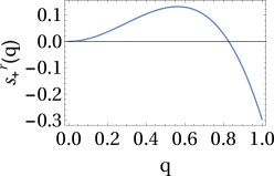
(a) (b)

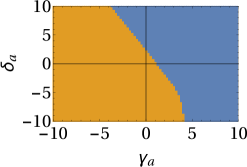
Figure 1: Linear stability analysis. (a) Plot of the real part of the largest growth rate $s_{+}^{r}(q)$ as a function of wave number $q$. All parameters are set equal to $1$ (including $\gamma_{\mathrm{a}}$ and $\delta_{\mathrm{a}}$), except $p_{0}=0.5$, $\xi=0.5$. We find $q_{\mathrm{max}}=\mathrm{argmax}_{q}(s_{+}^{r}(q))=0.56$, with a wave velocity $c=s_{+}^{i}(q_{\mathrm{max}})/q_{\mathrm{max}}=1.07$ greater than the mean tissue velocity $v_{0}=t_{\mathrm{a}}p_{0}/\xi=1$. We checked that $s_{-}^{r}(q)<0,\,\forall q$. (b) Bifurcation diagram in the $(\gamma_{\mathrm{a}},\delta_{\mathrm{a}})$ plane. The yellow (resp. blue) domain corresponds to a stable (resp. unstable) homogeneous state.

II.5 Summary

To summarize Eqs. (1-3) and (7-8), the dynamics is governed by a set of three coupled partial differential equations, with periodic boundary conditions on all fields:

$$\partial_{t}\rho+\partial_{x}(\rho v) = 0$$ (14)

$$-\partial_{x}\pi+\eta\;\partial^{2}_{x}v+\gamma_{\mathrm{a}}\;\partial_{x}\rho = \xi\,v-t_{\mathrm{a}}\,p$$ (15)

$$\partial_{t}p+v\,\partial_{x}p+\lambda\;p\,\partial_{x}v+\alpha_{\mathrm{a}}\;p\,\partial_{x}p = \Gamma_{\mathrm{p}}h+\delta_{\mathrm{a}}\;\partial_{x}\rho$$ (16)

where $h$ and $\pi$ are defined by (10) and (11) respectively.

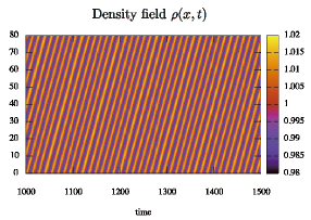
(a) (b)

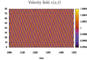
Figure 2: A traveling wave: all parameters are set equal to one $K=\rho_{\mathrm{e}}=a_{2}=\eta=\lambda=\Gamma_{p}=t_{\mathrm{a}}=\alpha_{\mathrm{a}}=\delta_{\mathrm{a}}=\gamma_{\mathrm{a}}=1$, except for $\xi=p_{0}=0.5$ and $K_{4}=0.0005$. The cell density (a) and velocity (b) kymographs are presented when $t\geq 1000$, after transients have died out. The polarity and stress fields also exhibit stable traveling wave solutions for the same parameter values (not shown).

III Linear stability analysis

The system (14-16), supplemented with (10-11) and (12-13) admits stationary, homogeneous solutions

$$(\rho,p,v)=(\rho_{0},p_{0},v_{0})$$

with finite polarity $p_{0}=\sqrt{a_{2}/a_{4}}$, finite velocity $v_{0}=t_{\mathrm{a}}p_{0}/\xi$, and arbitrary $\rho_{0}$. For simplicity, we set $\rho_{0}=\rho_{\mathrm{e}}$ in the following.

We study the growth rate $s$ of perturbations of wave number $q$:

$$(\rho,p,v)=(\rho_{\mathrm{e}},p_{0},v_{0})+(\delta\rho,\delta p,\delta v)\,e^{st-iqx}\,.$$ (17)

Substituting (17) into (14-16) with (10-11) and (12-13), we obtain to linear order a set of coupled equations, written in matrix form

$$\mathcal{L}\left(\begin{array}[]{c}\delta\rho\\ \delta p\\ \delta v\end{array}\right)=\left(\begin{array}[]{c}0\\ 0\\ 0\end{array}\right)$$ (18)

with

$$\mathcal{L}=\left(\begin{array}[]{ccc}s-iqv_{0}&0&-iq\rho_{\mathrm{e}}\\ iq\left(\frac{1}{K\rho_{\mathrm{e}}}-\gamma_{\mathrm{a}}+\nu\rho_{\mathrm{e}}q^{4}\right)&t_{\mathrm{a}}&-(\xi+\eta q^{2})\\ iq\delta_{\mathrm{a}}&s+2a_{2}\Gamma_{\mathrm{p}}-iq\left(v_{0}+\alpha_{\mathrm{a}}p_{0}\right)&-iq\lambda p_{0}\end{array}\right)$$

whose solution yields the wavenumber dependence of the complex-valued growth rates $s_{\pm}(q)=s_{\pm}^{r}(q)+is_{\pm}^{i}(q)$. A Hopf bifurcation occurs above a threshold value of a control parameter where the real part of the growth rate $s_{+}^{r}$ becomes positive, while its imaginary part is non-zero $s_{+}^{i}\neq 0$. For parameter values above threshold, the velocity of traveling waves is given by $c=s_{+}^{i}(q_{\mathrm{max}})/q_{\mathrm{max}}$, where $q_{\mathrm{max}}$ is the most unstable wavenumber $q_{\mathrm{max}}=\mathrm{argmax}_{q}(s_{+}^{r}(q))$.

We performed numerically the linear stability analysis. In Fig. 1a, we plot $s_{+}^{r}(q)$ with all parameter values set equal to one ($t_{\mathrm{a}}=\eta=\Gamma_{\mathrm{p}}=\lambda=K=\rho_{\mathrm{e}}=\alpha_{\mathrm{a}}=\delta_{\mathrm{a}}=\gamma_{\mathrm{a}}=1$), except $\xi=p_{0}=0.5$, and find that traveling waves are expected in this system, with a wave propagation velocity equal to $c=c(q_{\mathrm{max}})=1.07$, larger than the average velocity of the flow $v_{0}=1$. In Fig. 1b, we plot the bifurcation diagram in the $(\gamma_{\mathrm{a}},\delta_{\mathrm{a}})$ plane: a Hopf bifurcation occurs for large enough values of these active parameters.

From Eqs. (2-3), we deduce

$$-iq\delta\sigma=\xi\delta v-t_{\mathrm{a}}\delta p\,,$$

where the first term on the right hand side is dissipative. Eliminating $\delta\rho$ from (18), we find that, in the linear regime, $\delta p=(g^{r}(q)+ig^{i}(q))\,\delta v$, where $g^{r}$ and $g^{i}$ are real functions of the wavenumber, and obtain by substitution

$$-iq\delta\sigma=\left((\xi-t_{\mathrm{a}}g^{r}(q))-it_{\mathrm{a}}g^{i}(q)\right)\delta v\,.$$

The presence of an imaginary contribution $it_{\mathrm{a}}g^{i}(q)$ may explain the apparently “elastic” behaviour of the mechanical waves as presented in Serra-Picamal et al. (2012), while being in fact due to the active and polar nature of this compressible, viscous material (see a similar discussion in Blanch-Mercader and Casademunt (2017)).

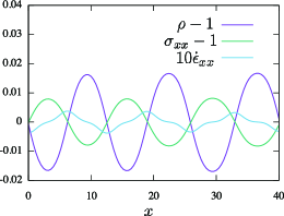
Figure 3: Spatial profiles of the density, stress and strain rate fields at $t=1000$. Parameter values are as in Fig. 2.

IV Numerical simulations

In this section, we present the results of numerical simulations of Eqs. (14-16), supplemented with (10-13). As an initial condition, we take the uniform state with $\rho=\rho_{\mathrm{e}}$, $p=p_{0}$, $v=v_{0}=t_{\mathrm{a}}p_{0}/\xi$ and add a noise of small amplitude. We used a finite-difference method and integrated Eqs. (14-16) on a discretized 1d space with mesh size $\Delta x=0.01$ and time step $\Delta t=0.0001$ as follows: Given the density field $\rho(x,t)$ and the polarity field $p(x,t)$ at a time step $t$, we solve Eq. (15) for the velocity field $v(x,t)$. Next, using Eq. (14) and Eq. (16), we determine the density field $\rho(x,t+\Delta t)$ and the polarity field $p(x,t+\Delta t)$ at the next time step $t+\Delta t$ with the explicit Euler method.

In Fig. 2, we set all parameters to one ($K=\rho_{\mathrm{e}}=a_{2}=\eta=\lambda=\Gamma_{p}=\gamma_{\mathrm{a}}=t_{\mathrm{a}}=\alpha_{\mathrm{a}}=\delta_{\mathrm{a}}=1$) except for $\xi=p_{0}=0.5$ and $K_{4}=0.0005$. As predicted by the linear stability analysis in the previous section, we confirm numerically that the instability occurs and the propagation velocity $(c\sim 1.07)$ is slightly larger than the mean tissue velocity $v_{0}=t_{\mathrm{a}}p_{0}/\xi=1$. The transient time scale is of the order of $10^{2}$. In Fig. 3, we show for the same parameter values the spatial profiles of the cell density, stress and strain rate $\dot{\epsilon}_{xx}=\partial_{x}v(x,t)$ at $t=1000$. The stress and strain rate are out-of-phase, while the stress and the cell density are in antiphase. If we consider that the cell area measured experimentally corresponds to the inverse of the cell density, both phase relations agree with experimental observations, which have been interpreted as evidence for an elastic rheology Serra-Picamal et al. (2012). However, our constitutive equation (7) is that of a compressible, viscous material, also endowed with active and polar properties.

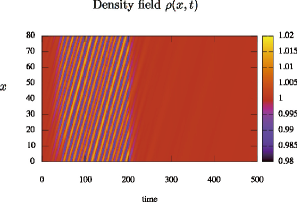
(a) (b)

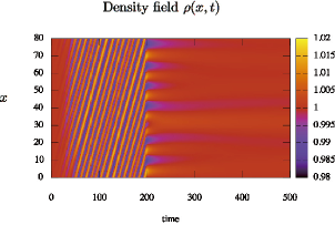
Figure 4: Numerical experiments mimicking inhibition assays: density kymographs, with parameters as in Fig. 2 until $t=200$. (a) Experimental inhibition of contractility by blebbistatin is mimicked by lowering the active parameters $\delta_{\mathrm{a}}$ and $\gamma_{\mathrm{a}}$ to $0.5$ when $t\geq 200$. (b) Experimental inhibition of Arp 2/3 is mimicked by lowering $p_{0}$ to a large negative value $-500$ when $t\geq 200$. In both cases the traveling wave pattern disappears when $t\geq 200$, as predicted by linear stability analysis.

Numerical simulations allow to mimic inhibition assays by tuning the value(s) of parameter(s) that would be changed due to the application of a drug. When we lower the value of the active parameters to $\delta_{\mathrm{a}}=0.5$, $\gamma_{\mathrm{a}}=0.5$ at $t=200$, we observe that the traveling wave rapidly disappears (see Fig. 4a), as observed experimentally when inhibiting contractility. In a similar manner, when we change the reference polarity value from a finite $p_{0}$ to $p_{0}=0$ (by setting $a_{2}=-500$ at $t=200$), the traveling waves also disappears quickly (see Fig. 4b), as observed experimentally when inhibiting Arp 2/3.

Finally, Fig. 5 shows an example of a traveling wave observed farther from threshold, with $\alpha_{\mathrm{a}}=2$, $\gamma_{\mathrm{a}}=\delta_{\mathrm{a}}=3$, and other parameters as in Fig. 2. The propagation velocity is accordingly larger $c\sim 1.3$.

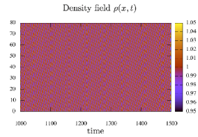
(a) (b)

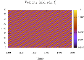
Figure 5: A traveling wave: Parameters are as in Fig. 2, except the active parameters $\alpha_{\mathrm{a}}=2$, $\gamma_{\mathrm{a}}=\delta_{\mathrm{a}}=3$. Kymographs of (a) the cell density (a); and (b) the velocity field are presented when $t\geq 1000$, after transients have died out. The polarity and stress fields also exhibit stable traveling wave solutions for the same parameter values (not shown).

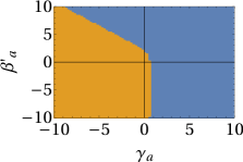
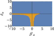
(a) (b) other parameter values are as in Fig. 1b. The yellow (resp. blue) domain corresponds to a stable (resp. unstable) homogeneous state.

Figure 6: Bifurcation diagrams: (a) in the $(\gamma_{\mathrm{a}},\beta^{\prime}_{\mathrm{a}})$ plane, with $\delta_{\mathrm{a}}=1$. (b) in the $(\beta^{\prime}_{\mathrm{a}},\delta_{\mathrm{a}})$ plane, with $\gamma_{\mathrm{a}}=1$. Our minimal model is supplemented with the $\beta^{\prime}_{\mathrm{a}}\;p^{2}$ term in (19), while

V Discussion

V.1 Robustness

Additional terms also invariant under simultaneous inversion of space and polarity are allowed by symmetry in the definition of the free energy density (9). A more complete, but also more complex expression of the free energy density as an expansion in terms of cell density, polarity, and their gradients reads

$$f=\, \psi_{\rho}(\rho)+\frac{K_{\rho}}{2}\;\left(\partial_{x}\rho\right)^{2}+\frac{\nu}{2}\,\left(\partial^{2}_{x}\rho\right)^{2}$$

$$+\varphi_{p}(p)+\frac{K_{\mathrm{F}}}{2}\;\left(\partial_{x}p\right)^{2}+\frac{\nu_{K}}{2}\,\left(\partial^{2}_{x}p\right)^{2}$$

$$+w_{1}\,\partial_{x}p+w_{2}\,\rho\,\partial_{x}p+w_{3}\,p\,\partial_{x}\rho+w_{4}\,\partial_{x}\rho\,\partial^{2}_{x}p+w_{5}\,\partial_{x}p\,\partial^{2}_{x}\rho+\ldots,$$

and is by no means exhaustive. It leads to more complex expressions of the conjugate fields $\pi$ and $h$. Here $K_{\mathrm{F}}\geq 0$ is Frank’s constant, the parameter $\nu_{K}\geq 0$ controls a term that further stabilizes large wavenumber modes, and the $w_{i}$’s couple density and polarity gradients. Note that the terms penalizing polarity gradients may become relevant in the presence of topological defects.

Similarly, additional nonlinear active terms could be included in the right hand side of (7):

$$\sigma=-\pi+\eta\;\partial_{x}v+\beta_{\mathrm{a}}\;\partial_{x}p+\beta^{\prime}_{\mathrm{a}}\;p^{2}+\sigma_{\mathrm{a}}+\gamma_{\mathrm{a}}\,\rho+\ldots$$ (19)

and of (8):

$$\dot{p}=\Gamma_{\mathrm{p}}\;h+a_{\emph{a}}\,p+a^{\prime}_{\emph{a}}\,\rho p-\lambda\;p\,\partial_{x}v-\alpha_{\mathrm{a}}\;p\,\partial_{x}p+\delta_{\mathrm{a}}\;\partial_{x}\rho+\ldots$$ (20)

since they also respect the invariance properties of $\sigma$ and $\dot{p}$.

We checked that these additional terms, while making the model more complex, do not change our qualitative conclusions: activity-driven traveling waves occur in large regions of the parameter space that govern active polar media (see also Giomi and Marchetti (2012); Ramaswamy and Jülicher (2016)). As an example motivated by Blanch-Mercader and Casademunt (2017), we add to our minimal model the $\beta^{\prime}_{\mathrm{a}}\;p^{2}$ term in (19), and show in Fig. 6 the resulting bifurcation diagrams in the $(\gamma_{\mathrm{a}},\beta^{\prime}_{\mathrm{a}})$ plane, at constant $\delta_{\mathrm{a}}$ and in the $(\beta^{\prime}_{\mathrm{a}},\delta_{\mathrm{a}})$ plane, at constant $\gamma_{\mathrm{a}}$ (compare with Fig. 1b).

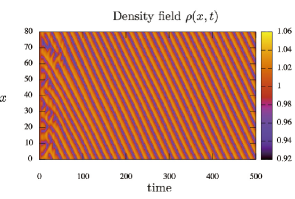
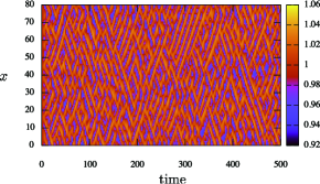
(a) (b) (c)

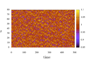
Figure 7: Secondary bifurcations. Our minimal model is supplemented with the $\beta^{\prime}_{\mathrm{a}}\;p^{2}$ term in (19), with parameters as in Fig. 2, except $a_{2}=-1$, $\beta_{\mathrm{a}}=0.1$, $\gamma_{\mathrm{a}}$, $\delta_{\mathrm{a}}$ and $\beta^{\prime}_{\mathrm{a}}$. Since $a_{2}<0$, the primary bifurcation is stationary. Density kymographs are shown, with (a) a traveling wave: $\gamma_{\mathrm{a}}=2$, $\delta_{\mathrm{a}}=4$ and $\beta^{\prime}_{\mathrm{a}}=20$; (b) coexistence of rightwards and leftwards traveling waves: $\gamma_{\mathrm{a}}=2$, $\delta_{\mathrm{a}}=4$ and $\beta^{\prime}_{\mathrm{a}}=30$; (c) a disordered pattern: $\gamma_{\mathrm{a}}=4$, $\delta_{\mathrm{a}}=8$ and $\beta^{\prime}_{\mathrm{a}}=20$.

V.2 Behaviour close to $p=0$

When the free energy is expanded close to $p=0$, bifurcations driven by the active parameters $\gamma_{\mathrm{a}}$ and $\delta_{\mathrm{a}}$ also occur. This case is obtained by setting $a_{2}<0$ in (12), and leads to substituting $p_{0}\to 0$, $v_{0}\to 0$ in (18). However, we find this time that $s_{+}^{i}(q_{\mathrm{max}})=0$, i.e. that the bifurcation is stationary and lead to standing waves. This is consistent with previous work on active polar materials Marcq (2014), and leads us to expect that traveling waves may then arise farther from threshold due to secondary bifurcations.

As an example, we show in Fig. 7 that a secondary bifurcation occurs in the presence of $\beta_{\mathrm{a}}$ and $\beta^{\prime}_{\mathrm{a}}$ : With the parameters $a_{2}=-1<0$, $\gamma_{\mathrm{a}}=2$, $\delta_{\mathrm{a}}=4$, $\beta_{\mathrm{a}}=0.1$ and $\beta^{\prime}_{\mathrm{a}}=20$, we found a travelling wave solution. When increasing $\beta^{\prime}_{\mathrm{a}}$ and fixing the other parameters, we observed that the stationary periodic pattern becomes unstable for $\beta^{\prime}_{\mathrm{a}}\gtrapprox 11.5$. We also obtained disordered patterns by further increasing the active parameters. The cases shown in Fig. 7 should be considered as examples. A full investigation of the complex spatio-temporal patterns generated by our model is left for future study.

V.3 Model comparison

A significant difference with the treatments proposed in Banerjee et al. (2015); Notbohm et al. (2016) is that we take into account the compressibility of the monolayer Zehnder et al. (2015, 2015) through the cell density balance equation (see Blanch-Mercader and Casademunt (2017) for an alternative way to treat incompressibility). Our formulation is more parsimonious than Banerjee et al. (2015); Notbohm et al. (2016) since we do not need to introduce an evolution equation for an additional chemical field in order to generate the instability. While the phenomenological model of wave generation proposed in Tlili et al. (2016) is based on a mechanotransduction pathway involving the protein Merlin Das et al. (2015), other authors favour the ERK Map kinase as a possible mechanochemical mediator Notbohm et al. (2016). Our approach does not depend upon a specific biochemical mechanism. It is based on general physical principles, notably symmetry arguments, which remain valid irrespective of the specific molecular mechanism at play. We propose a mechanism where activity couples to the cell density field. Only detailed comparison with experimental data is liable to determine which of the possible nonlinearities is involved.

Traveling waves are driven by either strong enough active stresses or strong enough active couplings in the evolution equation of the polarity field. As a consequence, their emergence does not depend on a specific rheology. Due to the 1D geometry, our choice of a rheology is somewhat ambiguous. According to Eq. (7), we assume that the epithelial rheology is that of a compressible, viscous fluid. Since it cancels at a finite value of the density, the pressure can also be interpreted in 1D as minus the elastic stress, $\pi=-\sigma_{\mathrm{el}}$. From this viewpoint, the epithelium rather behaves as a viscoelastic solid. An elastic behaviour corresponds to the limit of zero viscosity. Setting $\eta=0$ only shifts the instability threshold without altering the structure of the bifurcation diagram. Thus traveling waves arise in our model for a viscous, an elastic, and a viscoelastic rheology (Kelvin model). We conjecture that the equations one would write for a viscoelatic liquid (Maxwell model) would also give rise to activity-driven traveling waves Marcq (2014).

VI Conclusion

Within the framework of linear nonequilibrium thermodynamics, we wrote the constitutive equations for a one-dimensional, compressible, polar and active material, including lowest-order nonlinear active terms. We showed that Hopf bifurcations occur at threshold values of active parameters, leading to traveling waves for the relevant mechanical fields (density, velocity, polarity and stress). We thus formulated and justified a minimal, physical model of a tissue able to sustain traveling mechanical waves. A lower value of active parameters may suppress the waves, in agreement with experimental observation following the application of a drug inhibiting contractility. Switching to a state without a preferred polarity may also suppress the waves, just as inhibiting Arp 2/3 does in the cell monolayer. Not all epithelial cell types self-organize to generate traveling waves Vincent et al. (2015): in the light of our model, this suggests that active parameters are strongly cell-type dependent, and may accordingly be above or below the instability threshold.

In order to describe faithfully the experimental observations Serra-Picamal et al. (2012); Tlili et al. (2016), the model needs to be extended to a 2D geometry, and to include a moving free boundary in the numerical simulations, close to which polar order may be confined within a band of finite extension Blanch-Mercader et al. (2017). The same epithelial monolayers exhibit topological defects of the cell shape tensor field characteristic of a nematic material Saw et al. (2017). A more complete theory should take into account both types of orientational order.

References

- Cross and Hohenberg (1993) M. C. Cross and P. C. Hohenberg, Rev. Mod. Phys., 1993, 65, 851–1112.
- Meinhardt (2008) H. Meinhardt, Curr Top Dev Biol, 2008, 81, 1–63.
- ben Jacob et al. (2000) E. ben Jacob, I. Cohen and H. Levine, Adv. Physics, 2000, 49, 395 – 554.
- Kruse and Riveline (2011) K. Kruse and D. Riveline, Curr Top Dev Biol, 2011, 95, 67–91.
- Falcke (2003) M. Falcke, Adv. Phys., 2003, 53, 255–440.
- Karsenti (2008) E. Karsenti, Nat. Rev. Mol. Cell Biol., 2008, 9, 255–262.
- Beta and Kruse (2017) C. Beta and K. Kruse, Annu Rev Cond Matter Phys, 2017, 8, 239–264.
- Serra-Picamal et al. (2012) X. Serra-Picamal, V. Conte, R. Vincent, E. Anon, D. T. Tambe, E. Bazellieres, J. P. Butler, J. J. Fredberg and X. Trepat, Nat Phys, 2012, 8, 628–634.
- Tlili (2015) S. Tlili, PhD thesis, Université Paris Diderot, Paris, France, 2015.
- Tlili et al. (2016) S. Tlili, E. Gauquelin, B. Li, O. Cardoso, B. Ladoux, H. Delanoë-Ayari and F. Graner, arXiv:1610.05420, 2016.
- Notbohm et al. (2016) J. Notbohm, S. Banerjee, K. Utuje, B. Gweon, H. Jang, Y. Park, J. Shin, J. Butler, J. Fredberg and M. Marchetti, Biophys J, 2016, 110, 2729–2738.
- Poujade et al. (2007) M. Poujade, E. Grasland-Mongrain, A. Hertzog, J. Jouanneau, P. Chavrier, B. Ladoux, A. Buguin and P. Silberzan, Proc Natl Acad Sci USA, 2007, 104, 15988–15993.
- Vedula et al. (2012) S. R. K. Vedula, M. C. Leong, T. L. Lai, P. Hersen, A. J. Kabla, C. T. Lim and B. Ladoux, Proc Natl Acad Sci U S A, 2012, 109, 12974–12979.
- Cochet-Escartin et al. (2014) O. Cochet-Escartin, J. Ranft, P. Silberzan and P. Marcq, Biophys J, 2014, 106, 65–73.
- Bazellières et al. (2015) E. Bazellières, V. Conte, A. Elosegui-Artola, X. Serra-Picamal, M. Bintanel-Morcillo, P. Roca-Cusachs, J. J. M. noz, M. Sales-Pardo, R. Guimerà and X. Trepat, Nat Cell Biol, 2015, 17, 409–420.
- Lee and Wolgemuth (2011) P. Lee and C. W. Wolgemuth, PLoS Comput Biol, 2011, 7, e1002007.
- Köpf and Pismen (2012) M. H. Köpf and L. M. Pismen, Soft Matter, 2012, 9, 3727–3734.
- Recho et al. (2016) P. Recho, J. Ranft and P. Marcq, Soft Matter, 2016, 12, 2381–2391.
- Blanch-Mercader et al. (2017) C. Blanch-Mercader, R. Vincent, E. Bazellières, X. Serra-Picamal, X. Trepat and J. Casademunt, Soft Matter, 2017, 13, 1235–1243.
- Lee and Wolgemuth (2011) P. Lee and C. W. Wolgemuth, Phys Rev E, 2011, 83, 061920.
- Köpf and Pismen (2013) M. Köpf and L. Pismen, Physica D, 2013, 259, 48–54.
- Banerjee et al. (2015) S. Banerjee, K. Utuje and M. Marchetti, Phys Rev Lett, 2015, 114, 228101.
- Blanch-Mercader and Casademunt (2017) C. Blanch-Mercader and J. Casademunt, Soft Matter, 2017, in press.
- Zehnder et al. (2015) S. Zehnder, M. K. Wiatt, J. M. Uruena, A. C. Dunn, W. G. Sawyer and T. E. Angelini, Phys Rev E, 2015, 92, 032729.
- Zehnder et al. (2015) S. Zehnder, M. Suaris, M. M. Bellaire and T. E. Angelini, Biophys J, 2015, 108, 247–250.
- Guirao et al. (2015) B. Guirao, S. U. Rigaud, F. Bosveld, A. Bailles, J. López-Gay, S. Ishihara, K. Sugimura, F. Graner and Y. Bellaïche, Elife, 2015, 4, e08519.
- Yabunaka and Marcq (2016) S. Yabunaka and P. Marcq, Phys Rev E, 2017, in press.
- Chaikin and Lubensky (2000) P. Chaikin and T. Lubensky, Principles of Condensed Matter Physics, Cambridge University Press, 2000.
- Kruse et al. (2005) K. Kruse, J. Joanny, F. Jülicher, J. Prost and K. Sekimoto, Eur Phys J E, 2005, 16, 5–16.
- Marchetti et al. (2013) M. C. Marchetti, J. F. Joanny, S. Ramaswamy, T. B. Liverpool, J. Prost, M. Rao and R. A. Simha, Rev Mod Phys, 2013, 85, 1143–1189.
- Giomi and Marchetti (2012) L. Giomi and M. Marchetti, Soft Matter, 2012, 8, 129–139.
- Mindlin (1965) R. Mindlin, Int J Solid Struct, 1965, 1, 417–438.
- Ciarletta et al. (2012) P. Ciarletta, D. Ambrosi and G. Maugin, J Mech Phys Solids, 2012, 60, 432–450.
- Ramaswamy and Jülicher (2016) R. Ramaswamy and F. Jülicher, Sci Rep, 2016, 6, 20838.
- Marcq (2014) P. Marcq, Eur Phys J E, 2014, 37, 29.
- Das et al. (2015) T. Das, K. Safferling, S. Rausch, N. Grabe, H. Boehm and J. P. Spatz, Nat Cell Biol, 2015, 17, 276–287.
- Vincent et al. (2015) R. Vincent, E. Bazellières, C. Pérez-González, M. Uroz, X. Serra-Picamal and X. Trepat, Phys Rev Lett, 2015, 115, 248103.
- Saw et al. (2017) T. B. Saw, A. Doostmohammadi, V. Nier, L. Kocgozlu, S. Thampi, Y. Toyama, P. Marcq, C. T. Lim, J. M. Yeomans and B. Ladoux, Nature, 2017, 544, 212–216.